Consistency of the triplet seesaw model revisited

Abstract

Adding a scalar triplet to the Standard Model is one of the simplest ways of giving mass to neutrinos, providing at the same time a mechanism to stabilize the theory’s vacuum. In this paper, we revisit these aspects of the type-II seesaw model pointing out that the bounded-from-below conditions for the scalar potential in use in the literature are not correct. We discuss some scenarios where the correction can be significant and sketch the typical scalar boson profile expected by consistency.

March 13, 2024

1 Introduction

More than ever, after the discovery of the Higgs boson, particle physicists are eager for new results that can shed light on the symmetry breaking puzzle. The tiny neutrino masses suggest that probably a different mass generation scheme associated to their charge neutrality is at work. Neutrino masses can be introduced in the Standard Model (SM) through the lepton number violating coupling of a scalar triplet $\Delta$ (hypercharge $+1$) with the left-handed leptons,

$$\frac{Y_{\Delta,ij}}{2}L_{i}^{T}C\left(i\tau_{2}\right)\Delta L_{j}+\textrm{h.c.}$$ (1)

and generate a neutrino mass matrix $Y_{\Delta}\left\langle\Delta^{0}\right\rangle$ after electroweak symmetry breaking. Here $i\tau_{2}$ is the weak isospin conjugation matrix. The vacuum expectation value of the triplet is proportional to the strength $m_{H\Delta}$ of the coupling $HH\Delta$ which can be an arbitrarily small parameter since this is the only lepton number violating coupling in the model. This is arguably the most economical way of realizing Weinberg’ s dimension five operator [1]. For simplicity here we focus upon the case of explicit lepton number violation  [2] since the implementation of spontaneous lepton number violation  [3] would require an extended scalar sector containing also a singlet. In this scheme one “explains” the smallness of neutrino masses with the smallness of $m_{H\Delta}$ — and hence the smallness of the “induced” vacuum expectation value (VEV) $v_{\Delta}\equiv\left\langle\Delta^{0}\right\rangle$ — even with a light messenger scalar triplet $\Delta$, potentially accessible at the next run of the LHC.

On the other hand, it is known that the Higgs quartic coupling in the SM is driven to negative values at high energies, before the Planck scale is reached [4, 5]. With the triplet scalar field, the situation changes as the new quartic scalar interactions between $H$ and $\Delta$ are able to soften the decrease of the Higgs quartic coupling $\lambda_{H}$ as the energy scale is increased [6, 7, 8, 9]. The effect is qualitatively the same if the triplet is replaced by an $SU(2)_{L}$ singlet [10, 11, 12, 13, 14]. However, with the new triplet scalar, it is no longer enough to check that the Higgs quartic coupling stays positive, as the conditions for the potential to be bounded from below become more elaborate.

Regardless of the energy scale one may ask, under what conditions is the potential of the type-II seesaw model bounded from below? An attempt to write down for the first time these necessary and sufficient vacuum stability conditions taking into account all field directions has been made in [15]. However, as we point out in this paper, those conditions are too strong — they are sufficient but not necessary to ensure that a set of values for the quartic couplings corresponds to a stable vacuum. The structure of this paper is the following: after a brief review of the basic properties of the model (section 2) we derive the necessary and sufficient conditions for the potential to be bounded from below in section 3, discussing the difference with the conditions in use in the literature both from a theoretical point-of-view as well as a numerical one. In section 4 we apply these conditions to explore the region in parameter space of the type-II seesaw where the potential is stable up to some given scale. Finally, we present some conclusions in section 6. (Two appendices provide supplementary material.)

2 Basic properties of the type-II seesaw model

Here we consider the simplest neutrino mass generation scheme based on an effective seesaw mechanism with explicit lepton number violation described by the complex triplet, given as

$$\Delta\equiv\left(\begin{array}[]{cc}\frac{\Delta^{+}}{\sqrt{2}}&\Delta^{++}\\ \Delta^{0}&-\frac{\Delta^{+}}{\sqrt{2}}\end{array}\right) \,.$$ (4)

The most general potential involving $\Delta$ and the Standard Model Higgs doublet $H=\left(H^{+},H^{0}\right)^{T}$ has a total of eight parameters which we can take to be real:

$$V\left(H,\Delta\right) =-\mu_{H}^{2}H^{\dagger}H+\mu_{\Delta}^{2}\textrm{Tr}\left(\Delta^{\dagger}\Delta\right)+\left[\frac{m_{H\Delta}}{2}H^{T}\left(i\tau_{2}\right)\Delta^{\dagger}H+\textrm{h.c.}\right]+\frac{1}{2}\lambda_{H}\left(H^{\dagger}H\right)^{2}$$

$$+\lambda_{H\Delta}\textrm{Tr}\left(\Delta^{\dagger}\Delta\right)\left(H^{\dagger}H\right)+\lambda^{\prime}_{H\Delta}H^{\dagger}\Delta\Delta^{\dagger}H+\frac{\lambda_{\Delta}}{2}\left[\textrm{Tr}\left(\Delta^{\dagger}\Delta\right)\right]^{2}+\frac{\lambda^{\prime}_{\Delta}}{2}\textrm{Tr}\left(\Delta^{\dagger}\Delta\Delta^{\dagger}\Delta\right)\,.$$ (5)

The vacuum expectation value of the neutral component of the triplet, $v_{\Delta}\equiv\left\langle\Delta^{0}\right\rangle$, must be significantly smaller than the one of the standard Higgs, $v_{H}\equiv\left\langle H^{0}\right\rangle$, otherwise the $\rho$ parameter will deviate too much from 1. Indeed,

$$\rho \approx 1-2\alpha^{2}$$ (6)

with $\alpha\equiv v_{\Delta}/v_{H}$ so this ratio of VEVs can be at most of the percent order given the experimental constraints on $\rho$ [16]. Furthermore, since neutrino masses are proportional to $v_{\Delta}$, this VEV should indeed be very small. Under the approximation that $\alpha\ll 1$, the minimization solution of the potential requires that

$$\mu_{H}^{2} \approx\lambda_{H}v_{H}^{2}\,,$$ (7)

$$\mu_{\Delta}^{2} \approx\left(\frac{\chi}{2}-\lambda_{H\Delta}-\lambda^{\prime}_{H\Delta}\right)v_{H}^{2}\,,$$ (8)

where

$$\chi\equiv m_{H\Delta}/v_{\Delta}.$$ (9)

Using these relations one can write the scalar boson mass eigenstates as shown in table 1.

Mass eigenstate $\phi$	Mass squared $m_{\phi}^{2}$	Composition
$H^{++}$	$v_{H}^{2}\left(\frac{\chi}{2}-\lambda^{\prime}_{H\Delta}\right)$	$\Delta^{++}$
$G^{+}$	$0$	$H^{+}+\sqrt{2}\alpha\Delta^{+}$
$H^{+}$	$v_{H}^{2}\left(\frac{\chi}{2}-\frac{\lambda^{\prime}_{H\Delta}}{2}\right)$	$\Delta^{+}-\sqrt{2}\alpha H^{+}$
$G^{0}$	$0$	$H_{I}^{0}+2\alpha\Delta_{I}^{0}$
$A^{0}$	$\frac{1}{2}v_{H}^{2}\chi$	$\Delta_{I}^{0}-2\alpha H_{I}^{0}$
$h^{0}$	$2\lambda_{H}v_{H}^{2}$	$H_{R}^{0}+2\alpha\frac{\chi-2\lambda_{H\Delta}-2\lambda^{\prime}_{H\Delta}}{\chi-4\lambda_{H}}\Delta_{R}^{0}$
$H^{0}$	$\frac{1}{2}v_{H}^{2}\chi$	$\Delta_{R}^{0}-2\alpha\frac{\chi-2\lambda_{H\Delta}-2\lambda^{\prime}_{H\Delta}}{\chi-4\lambda_{H}}H_{R}^{0}$

Table 1: Scalar mass eigenstates in the type-II seesaw model. We have defined the dimensionless parameters $\alpha\equiv v_{\Delta}/v_{H}$ and $\chi\equiv m_{H\Delta}/v_{\Delta}$.

Note that if the doubly charged Higgs $H^{++}$ is to be heavier than half a TeV or so, then $\chi\apprge 10$, making $\chi$ significantly larger than any of the quartic couplings $\lambda_{i}$ which one expects to be, at most, of order 1. Moreover, one sees that for a suitable $\chi$ the would-be triplet Nambu-Goldstone boson state $A^{0}$ can be massive enough to have escaped detection at LEP.

3 When is the scalar potential bounded from below?

We now turn to the important issue of the stability of the VEV solution mentioned above. As long as all scalar masses are positive, the potential will not roll down classically to another minimum, but this still leaves open the possibility of a tunneling to a deeper minimum. In order for this not to happen, it is necessary (although not sufficient) that the potential does not fall to infinitely negative values in any VEV direction. In other words, we must ensure that $V$ is bounded from below, which is equivalent to the requirement that the quartic part of the potential in equation (5), $V^{(4)}$, must be positive for all non-zero field values. In the following then, we shall derive the necessary and sufficient conditions for this to be true, correcting the result obtained in [15].

While there are ten real degrees of freedom (four in $H$ plus six in $\Delta$), $V$ depends on them only through 4 quantities: $H^{\dagger}H$, $\textrm{Tr}\left(\Delta^{\dagger}\Delta\right)$, $H^{\dagger}\Delta\Delta^{\dagger}H$ and $\textrm{Tr}\left(\Delta^{\dagger}\Delta\Delta^{\dagger}\Delta\right)$. In the following, we shall take $\textrm{Tr}\left(\Delta^{\dagger}\Delta\right)$ to be non-zero. We now define $r$, $\zeta$ and $\xi$ as the following non-negative dimensionless quantities [15],

$$H^{\dagger}H \equiv r\textrm{Tr}\left(\Delta^{\dagger}\Delta\right)\,,$$ (10)

$$\textrm{Tr}\left(\Delta^{\dagger}\Delta\Delta^{\dagger}\Delta\right) \equiv\zeta\left[\textrm{Tr}\left(\Delta^{\dagger}\Delta\right)\right]^{2}\,,$$ (11)

$$H^{\dagger}\Delta\Delta^{\dagger}H \equiv\xi\textrm{Tr}\left(\Delta^{\dagger}\Delta\right)\left(H^{\dagger}H\right)\,,$$ (12)

such that the quartic part of the potential reads

$$\frac{V^{(4)}}{\left[\textrm{Tr}\left(\Delta^{\dagger}\Delta\right)\right]^{2}} =\frac{1}{2}\lambda_{H}r^{2}+\lambda_{H\Delta}r+\lambda^{\prime}_{H\Delta}\xi r+\frac{\lambda_{\Delta}}{2}+\frac{\lambda^{\prime}_{\Delta}}{2}\zeta\,.$$ (13)

This expression must be positive for all allowed values of $r$, $\zeta$ and $\xi$. Consider first $r$: from equation (10) it is clear that $r$ can take any non-negative value which means that, given the quadratic dependence of equation (13) on $r$ that one must have

$$0 <\lambda_{H}\,,$$ (14)

$$0 <\lambda_{\Delta}+\lambda^{\prime}_{\Delta}\zeta\equiv F_{1}\left(\zeta\right)\,,$$ (15)

$$0 <\lambda_{H\Delta}+\xi\lambda^{\prime}_{H\Delta}+\sqrt{\lambda_{H}\left(\lambda_{\Delta}+\lambda^{\prime}_{\Delta}\zeta\right)}\equiv F_{2}\left(\xi,\zeta\right)\,.$$ (16)

These conditions match those given in [15] with a different notation. However, what follows differs with [15] in a crucial way.

In order to obtain the necessary and sufficient conditions for the quartic couplings $\lambda_{i}$ which yield a potential bounded from below, one needs to get rid of $\zeta$ and $\xi$ from conditions (14)–(16). Note that these conditions must be respected for all $\zeta$ and $\xi$, so one needs to find what are the allowed values of $\left(\xi,\zeta\right)$ from the definition of these two quantities. We do not show the details here, but the reader can convince her/himself that $\xi$ can take any value between $0$ and $1$ and $\zeta$ can be anywhere between $1/2$ and 1, as noted in [15].

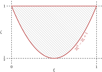
Figure 1: The shaded region is the allowed one for the parameters $\left(\xi,\zeta\right)$.

However, the crucial point is that this does not mean that $\left(\xi,\zeta\right)$ can be anywhere in the rectangle with vertices in $\left(0,\frac{1}{2}\right)$ and $\left(1,1\right)$. Indeed, from equations (11) and (12) it can be shown that the possible values of $\left(\xi,\zeta\right)$ correspond to

$$2\xi^{2}-2\xi+1\leq\zeta\leq 1\,,$$ (17)

which defines the shaded region depicted in figure 1. Since the function $F_{1}\left(\zeta\right)$ defined in (15) is monotonic, the condition ‘$0<F_{1}\left(\zeta\right)$ for all $\zeta$’ is equivalent to ‘$0<F_{1}\left(\frac{1}{2}\right)$ and $0<F_{1}\left(1\right)$’ which translates into the requirement

$$0<\lambda_{\Delta}+\frac{1}{2}\lambda^{\prime}_{\Delta}\textrm{ and }0<\lambda_{\Delta}+\lambda^{\prime}_{\Delta}\,.$$ (18)

As for the condition in (16), note that ‘$0<F_{2}\left(\xi,\zeta\right)$ for all $\xi$ and $\zeta$’ is trivially the same as $0<\min F_{2}\left(\xi,\zeta\right)$, so one is left with the job of finding the minimum of $F_{2}$. Furthermore, since this function is monotonic in both $\xi$ and $\zeta$, we know that its minimum occurs at the border of the shaded region in figure 1; to be more specific, this argument shows that the minimum of the function must occur somewhere along the line defined by $\zeta=2\xi^{2}-2\xi+1$, with $0\leq\xi\leq 1$. Then we may take

$$\widehat{F}\left(\xi\right) \equiv F_{2}\left(\xi,2\xi^{2}-2\xi+1\right)$$ (19)

noticing that the sign of $\widehat{F}^{\prime\prime}\left(\xi\right)$ is constant — it is the same as the one of $\lambda^{\prime}_{\Delta}$. Therefore, one can always find a value $\xi_{0}$ where $\widehat{F}^{\prime}\left(\xi_{0}\right)=0$. Such a $\xi_{0}$ will be a minimum if $\widehat{F}^{\prime\prime}\left(\xi_{0}\right)>0$ and, furthermore, one must also make sure that $0\leq\xi_{0}\leq 1$ (or equivalently that $\widehat{F}^{\prime}\left(0\right)<0$ and $\widehat{F}^{\prime}\left(1\right)>0$ since $\widehat{F}^{\prime}$ is a monotonous function). This will be true if and only if $\lambda^{\prime}_{\Delta}\sqrt{\lambda_{H}}>\left|\lambda^{\prime}_{H\Delta}\right|\sqrt{\lambda_{\Delta}+\lambda^{\prime}_{\Delta}}$, in which case

$$\widehat{F}\left(\xi_{0}\right) =\lambda_{H\Delta}+\frac{1}{2}\lambda^{\prime}_{H\Delta}+\frac{1}{2}\sqrt{\left(2\lambda_{H}\lambda^{\prime}_{\Delta}-{\lambda^{\prime}_{H\Delta}}^{2}\right)\left(2\frac{\lambda_{\Delta}}{\lambda^{\prime}_{\Delta}}+1\right)}\,.$$ (20)

The remaining possibility is that the minimum of $\widehat{F}$ in the interval $\xi\in\left[0,1\right]$ is at $\xi=0$ or $1$, from which we get the constraints that both $\widehat{F}\left(0\right)=\lambda_{H\Delta}+\sqrt{\lambda_{H}\left(\lambda_{\Delta}+\lambda^{\prime}_{\Delta}\right)}$ and $\widehat{F}\left(1\right)=\lambda_{H\Delta}+\lambda^{\prime}_{H\Delta}+\sqrt{\lambda_{H}\left(\lambda_{\Delta}+\lambda^{\prime}_{\Delta}\right)}$ should be positive quantities.

In summary, the potential will be bounded from below if and only if

$$\lambda_{H},\,\lambda_{\Delta}+\lambda^{\prime}_{\Delta},\,\lambda_{\Delta}+\frac{1}{2}\lambda^{\prime}_{\Delta},\,\lambda_{H\Delta}+\sqrt{\lambda_{H}\left(\lambda_{\Delta}+\lambda^{\prime}_{\Delta}\right)},\,\lambda_{H\Delta}+\lambda^{\prime}_{H\Delta}+\sqrt{\lambda_{H}\left(\lambda_{\Delta}+\lambda^{\prime}_{\Delta}\right)}>0$$

and

$$\left[\lambda^{\prime}_{\Delta}\sqrt{\lambda_{H}}\leq\left|\lambda^{\prime}_{H\Delta}\right|\sqrt{\lambda_{\Delta}+\lambda^{\prime}_{\Delta}}\textrm{ or }2\lambda_{H\Delta}+\lambda^{\prime}_{H\Delta}+\sqrt{\left(2\lambda_{H}\lambda^{\prime}_{\Delta}-{\lambda^{\prime}_{H\Delta}}^{2}\right)\left(2\frac{\lambda_{\Delta}}{\lambda^{\prime}_{\Delta}}+1\right)}>0\right]\,.$$ (21)

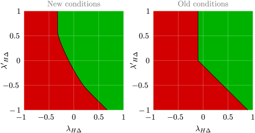
Figure 2: Regions of stability (green) and instability (red) of the potential for $\lambda_{\Delta}=-\frac{1}{3}$, $\lambda^{\prime}_{\Delta}=\frac{3}{4}$ and $\lambda_{H}\approx\frac{1}{4}$. The two plots make it possible to compare the correct stability conditions as given in equation (22) (left) with the ones in use in the literature (right).

The condition in (21) should be compared with the one used up to now in the literature, where the last line of (21) is replaced by $F_{2}\left(0,\frac{1}{2}\right),\,F_{2}\left(1,\frac{1}{2}\right)>0$, which translates into

$$\lambda_{H\Delta}+\sqrt{\lambda_{H}\left(\lambda_{\Delta}+\frac{1}{2}\lambda^{\prime}_{\Delta}\right)},\,\lambda_{H\Delta}+\lambda^{\prime}_{H\Delta}+\sqrt{\lambda_{H}\left(\lambda_{\Delta}+\frac{1}{2}\lambda^{\prime}_{\Delta}\right)}>0\,.$$ (22)

From the discussion so far it should be clear that this condition is too strict: potentials $V$ which obey it are necessarily bounded from below, but not all potentials which are bounded from below do obey it. Indeed, the constraint in (22) assumes that by varying the fields $H$ and $\Delta$ the point $\left(\xi,\zeta\right)$ can be anywhere within the dashed rectangle in figure 1, when in reality only the shaded region is allowed, with two thirds of the area of the rectangle. Restricting to the 5-dimensional box region where $\left|\lambda_{i}\right|\leq 1$, a numerical scan indicates that close to 5% of the valid points are excluded by the constraint in (22), although in certain special scenarios, as in figure 2, this percentage can be significantly larger.

4 Regions of stability and perturbativity

Now that we have the correct stability conditions we consider the renormalization group evolution of the triplet seesaw model. Ignoring all Yukawa couplings except the one of the top, using [17, 18, 19] one finds the renormalization group equations of the model to be the following (see also [20, 21]):

$$\left(4\pi\right)^{2}\frac{dg_{i}}{dt} =b_{i}g_{i}^{3}\textrm{ with }b_{i}=\left(\frac{47}{10},-\frac{5}{2},-7\right)\,,$$ (23)

$$\left(4\pi\right)^{2}\frac{d\lambda_{H}}{dt} =\frac{27}{100}g_{1}^{4}+\frac{9}{10}g_{1}^{2}g_{2}^{2}+\frac{9}{4}g_{2}^{4}-\left(\frac{9}{5}g_{1}^{2}+9g_{2}^{2}\right)\lambda_{H}+12\lambda_{H}^{2}+6\lambda_{H\Delta}^{2}+6\lambda_{H\Delta}\lambda^{\prime}_{H\Delta}+\frac{5}{2}{\lambda^{\prime}_{H\Delta}}^{2}$$

$$+12\lambda_{H}y_{t}^{2}-12y_{t}^{4}\,,$$ (24)

$$\left(4\pi\right)^{2}\frac{d\lambda_{H\Delta}}{dt} =\frac{27}{25}g_{1}^{4}-\frac{18}{5}g_{1}^{2}g_{2}^{2}+6g_{2}^{4}-\left(\frac{9}{2}g_{1}^{2}+\frac{33}{2}g_{2}^{2}\right)\lambda_{H\Delta}+6\lambda_{H}\lambda_{H\Delta}+2\lambda_{H}\lambda^{\prime}_{H\Delta}+4\lambda_{H\Delta}^{2}$$

$$+8\lambda_{\Delta}\lambda_{H\Delta}+6\lambda^{\prime}_{\Delta}\lambda_{H\Delta}+{\lambda^{\prime}_{H\Delta}}^{2}+3\lambda_{\Delta}\lambda^{\prime}_{H\Delta}+\lambda^{\prime}_{\Delta}\lambda^{\prime}_{H\Delta}+6\lambda_{H\Delta}y_{t}^{2}\,,$$ (25)

$$\left(4\pi\right)^{2}\frac{d\lambda^{\prime}_{H\Delta}}{dt} =\frac{36}{5}g_{1}^{2}g_{2}^{2}-\left(\frac{9}{2}g_{1}^{2}+\frac{33}{2}g_{2}^{2}\right)\lambda^{\prime}_{H\Delta}+2\lambda_{H}\lambda^{\prime}_{H\Delta}+8\lambda_{H\Delta}\lambda^{\prime}_{H\Delta}+4{\lambda^{\prime}_{H\Delta}}^{2}+2\lambda_{\Delta}\lambda^{\prime}_{H\Delta}$$

$$+4\lambda^{\prime}_{\Delta}\lambda^{\prime}_{H\Delta}+6\lambda^{\prime}_{H\Delta}y_{t}^{2}\,,$$ (26)

$$\left(4\pi\right)^{2}\frac{d\lambda_{\Delta}}{dt} =\frac{108}{25}g_{1}^{4}-\frac{72}{5}g_{1}^{2}g_{2}^{2}+30g_{2}^{4}-\left(\frac{36}{5}g_{1}^{2}+24g_{2}^{2}\right)\lambda_{\Delta}+4\lambda_{H\Delta}^{2}+4\lambda_{H\Delta}\lambda^{\prime}_{H\Delta}$$

$$+14\lambda_{\Delta}^{2}+12\lambda_{\Delta}\lambda^{\prime}_{\Delta}+3{\lambda^{\prime}_{\Delta}}^{2}\,,$$ (27)

$$\left(4\pi\right)^{2}\frac{d\lambda^{\prime}_{\Delta}}{dt} =\frac{144}{5}g_{1}^{2}g_{2}^{2}-12g_{2}^{4}+2{\lambda^{\prime}_{H\Delta}}^{2}-\left(\frac{36}{5}g_{1}^{2}+24g_{2}^{2}\right)\lambda^{\prime}_{\Delta}+12\lambda_{\Delta}\lambda^{\prime}_{\Delta}+9{\lambda^{\prime}_{\Delta}}^{2}\,.$$ (28)

Using these equations and requiring stability of the scalar potential in the energy range going from the top mass all the way to the Planck mass one obtains the regions of quartic couplings indicated in green in figure 3. The right panel corresponds to the use of the stability conditions used in the literature, while the left panel refers to our new and less restrictive stability conditions. On the other hand the instability regions are indicated in red. Finally those cases which correspond to a stable vacuum but involve non-perturbative dynamics because $\left|\lambda_{i}\right|>\sqrt{4\pi}$ for some quartic coupling $\lambda_{i}$ are indicated in orange. Notice also that the stable region becomes bigger if one imposes stability only up to some intermediate scale, chosen to be $10^{12}$ GeV, as indicated by the light green region in figure 3.

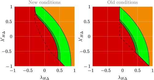
Figure 3: Regions of stability (dark green) and instability (red) considering the energy range going from the top mass all the way to the Planck mass. Those cases which (appear to) lead to a stable vacuum but involve non-perturbative dynamics because $\left|\lambda_{i}\right|>\sqrt{4\pi}$ for some quartic coupling $\lambda_{i}$ are shown in orange. If one requires stability only up to $10^{12}$ GeV the stable region becomes bigger, as indicated by the light green region. The dashed lines indicate the border between the stable and unstable regions at low energies (see figure 2).

5 Phenomenological profile of the triplet seesaw Higgs sector

Since its original proposal there have been many phenomenological studies of the scalar sector of the triplet model, as it constitutes an essential ingredient of the type-II seesaw mechanism. For the benefit of the reader we present in figure 5 of Appendix B a schematic view of the scalar boson mass spectrum in the model given in table 1. One sees that, in addition to the SM Higgs boson found, one has heavy neutral ($H^{0}$,$A^{0}$), singly ($H^{+}$) and doubly charged ($H^{++}$) scalar bosons, whose mass is controlled by $\chi$ and with a small splitting which should not be bigger than indicated on figure 4 if the model is to remain perturbative all the way up to the Planck scale.

The doubly–charged state comes just from the triplet, while all other heavy states come mainly from the triplet, but with a small admixture with the standard model Higgs boson, controlled by the ratio of VEVs $\alpha\equiv v_{\Delta}/v_{H}$. Note that the state $A^{0}$ is identified with the would-be triplet Nambu-Goldstone boson associated to spontaneous lepton number violation which becomes massless as $v_{\Delta}\to 0$. All of these scalar states have a nearly common mass, with a small splitting, both indicated in figure 5. This follows from the consistency requirements such as perturbativity studied in the previous section and displayed in figure 4. Hence, altogether, once the lightest Higgs boson discovered at the LHC is accommodated, one can describe fairly well the scalar sector with just three parameters ($\alpha$, $\lambda^{\prime}_{H\Delta}$ and $\chi$). This is in sharp contrast with other extended electroweak breaking potentials, such as those of supersymmetric models.

For example the singly and doubly–charged members of the triplet have been searched for at accelerators such as LEP as well as hadron colliders  [22, 23, 24, 25]. If sufficiently light, say below 400 GeV or so, the $H^{++}$ will be copiously produced at the LHC, which could enable interesting measurements of its branching ratios of the various leptonic decay channels [26], as well as the leading $WW$ decay branch [27, 28]. The former are determined by the triplet Yukawa couplings. These determine also the pattern of lepton flavour violation decays. Given the small neutrino masses indicated by experiment [29, 30, 31, 32] and our assumption that the scalars are in the TeV region, these Yukawa couplings are expected to be too small to cause detectable signals.

The near degeneracy of the heavy scalars implies that, once the constraints on the charged Higgs bosons are imposed, by choosing a suitably large $\chi$, the neutral ones, including the would–be Majoron, will also have escaped detection at LEP. Moreover, the charged components in the Higgs triplet model provide a potential enhancement of the $H\to\gamma\gamma$ decay branching [33, 34, 8] ratio, which can be probed at the LHC. Last but not least, the triplet introduces changes to the $S,T,U$ oblique parameters.

All of the above phenomena should be studied within parameter regions where the electroweak symmetry breaking is consistent and, as we saw in figure 3, consistency implies strong restrictions on quartic parameter values. Although the relevant restrictions apply mainly to the quartic scalar interactions, and in principle do not translate directly into stringent constraints upon the Higgs boson masses, one has an important restriction on the splitting between the masses of the heavy states, such as the singly and doubly charged scalar bosons, illustrated by the funnel region depicted in figure 4. Performing a dedicated phenomenological study of the scalar sector lies outside the scope of this paper but we hope to have given a helpful guideline.

One last word regarding the naturalness of the scalar potential in the presence of the cubic mass parameter. This follows from the principle that its removal would lead to a theory of enhanced symmetry, in which neutrinos would be massless and lepton number would be conserved. In any case, a dynamical completion of this theory in which the cubic term is replaced by a quartic one is possible and has in fact been suggested long ago [3]. This would imply the presence of a mainly singlet Nambu-Goldstone boson with implications for Higgs decays such as invisibly decaying Higgs bosons [35, 36, 37] whose detailed analysis is more general than the one recently given in reference [14] and lies outside the scope of the present paper.

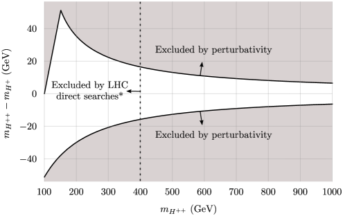
Figure 4: The coupling $\lambda^{\prime}_{H\Delta}$ must be roughly between -0.85 and 0.85 if all quartic couplings are to remain small up to $m_{Planck}$ ($\left|\lambda_{i}\right|<\sqrt{4\pi}$). This perturbativity requirement strongly constrains the mass splitting of the triplet components, particularly if one considers the LHC lower bound $m_{H^{++}}\sim 400$ GeV from direct searches of $H^{++}$ decaying in to leptons [24, 25] (*assuming 100% branching fractions). This plot also assumes that $m_{H^{+}}>100$ GeV.

6 Final remarks

In this paper, we have considered the consistency of the type-II seesaw model symmetry breaking. We included under consistency both the requirements of boundedness from below as well as perturbativity up to some scale. We found that the bounded-from-below conditions for the scalar potential in use in the literature are not correct. For definiteness and simplicity we focused on the case of explicit violation of lepton number. We discussed some scenarios where the correction we have found can be significant. Moreover we have sketched the typical scalar boson profile expected by consistency of the vacuum. Before closing we note that, the restrictions discussed in this paper do not depend on the hypercharge of the scalar triplet $\Delta$, hence the same set of conditions also applies for any other model which extends the scalar sector of the Standard Model with an $SU(2)_{L}$ triplet.

Acknowledgments

This work supported by the Spanish grants FPA2014-58183-P, Multidark CSD2009-00064 and SEV-2014-0398 (MINECO), and PROMETEOII/2014/084 (Generalitat Valenciana).

Appendix A: Conversion between different notations

Given that different notations are used in the literature to write down the different terms in the scalar potential of the model, we provide here table 2 to facilitate comparisons.

Source	$\mu_{H}^{2}$	$\mu_{\Delta}^{2}$	$m_{H\Delta}$	$\lambda_{H}$	$\lambda_{H\Delta}$	$\lambda^{\prime}_{H\Delta}$	$\lambda_{\Delta}$	$\lambda^{\prime}_{\Delta}$
[15]	$m_{H}^{2}$	$M_{\Delta}^{2}$	$\frac{1}{2}\mu$	$\frac{1}{2}\lambda$	$\lambda_{1}$	$\lambda_{4}$	$2\lambda_{2}$	$2\lambda_{3}$
[8]*	$-m^{2}$	$M^{2}$	$\sqrt{2}\mu$	$2\lambda_{1}$	$\lambda_{4}-\lambda_{5}$	$2\lambda_{5}$	$2\lambda_{2}+2\lambda_{3}$	$-2\lambda_{3}$
[20]*	$-m_{\phi}^{2}$	$M_{\xi}^{2}$	$-\left(\lambda_{H}M_{\xi}\right)^{*}$	$\frac{1}{2}\lambda$	$\lambda_{\phi}-\frac{1}{2}\lambda_{T}$	$\lambda_{T}$	$4\lambda_{C}+\frac{1}{2}\lambda_{\xi}$	$-4\lambda_{C}$
[9]*	$-m_{\Phi}^{2}$	$M_{\Delta}^{2}$	$\sqrt{2}\Lambda_{6}$	$\lambda$	$\lambda_{4}+\lambda_{5}$	$-2\lambda_{5}$	$\lambda_{1}+\lambda_{2}$	$-\lambda_{2}$

Table 2: Translation between the notation used in this paper and the one used by other authors. Note that in the cases marked with an asterisk it is also necessary to flip the sign of the doubly charged component of the triplet.

Appendix B: Representative triplet seesaw scalar mass spectrum

In order to grasp in a visual manner the scalar spectrum of the model (see table 1) as well as the effect on the degeneracy of the three new scalars of having $\lambda^{\prime}_{H\Delta}$ constrained to be roughly between -0.85 and 0.85, we present here figure 5.

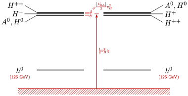
Figure 5: Schematic view of the scalar boson mass spectrum in the triplet seesaw model. The heavy scalars are nearly degenerate. The ordering of the heavy scalar masses depends on the sign of $\lambda^{\prime}_{H\Delta}$ as shown in table 1. Recall that $\chi$ refers to the ratio $m_{H\Delta}/v_{\Delta}$.

References

- [1] S. Weinberg, Varieties of baryon and lepton nonconservation, Phys. Rev. D22 (1980) 1694.
- [2] J. Schechter and J. Valle, Neutrino masses in theories, Phys.Rev. D22 (1980) 2227.
- [3] J. Schechter and J. W. F. Valle, Neutrino decay and spontaneous violation of lepton number, Phys. Rev. D25 (1982) 774.
- [4] M. Sher, Electroweak Higgs potentials and vacuum stability, Phys. Rept. 179 (1989) 273–418.
- [5] S. Alekhin, A. Djouadi and S. Moch, The top quark and Higgs boson masses and the stability of the electroweak vacuum, Phys. Lett. B716 (2012) 214–219, arXiv:1207.0980 [hep-ph].
- [6] I. Gogoladze, N. Okada and Q. Shafi, Higgs boson mass bounds in a type II seesaw model with triplet scalars, Phys. Rev. D78 (2008) 085005, arXiv:0802.3257 [hep-ph].
- [7] W. Chao, M. Gonderinger and M. J. Ramsey-Musolf, Higgs vacuum stability, neutrino mass, and dark matter, Phys. Rev. D86 (2012) 113017, arXiv:1210.0491 [hep-ph].
- [8] E. J. Chun, H. M. Lee and P. Sharma, Vacuum stability, perturbativity, EWPD and Higgs-to-diphoton rate in type II seesaw models, JHEP 11 (2012) 106, arXiv:1209.1303 [hep-ph].
- [9] P. Bhupal Dev, D. K. Ghosh, N. Okada and I. Saha, 125 GeV Higgs boson and the type-II seesaw model, JHEP 1303 (2013) 150, arXiv:1301.3453 [hep-ph].
- [10] O. Lebedev, On stability of the electroweak vacuum and the Higgs portal, Eur. Phys. J. C72 (2012) 2058, arXiv:1203.0156 [hep-ph].
- [11] J. Elias-Miro et al., Stabilization of the electroweak vacuum by a scalar threshold effect, JHEP 06 (2012) 031, arXiv:1203.0237 [hep-ph].
- [12] A. Falkowski, C. Gross and O. Lebedev, A second Higgs from the Higgs portal, JHEP 05 (2015) 057, arXiv:1502.01361 [hep-ph].
- [13] R. Costa, A. P. Morais, M. O. P. Sampaio and R. Santos, Two-loop stability of a complex singlet extended Standard Model, Phys. Rev. D92 (2015) 2 025024, arXiv:1411.4048 [hep-ph].
- [14] C. Bonilla, R. M. Fonseca and J. W. F. Valle, Vacuum stability with spontaneous violation of lepton number (2015), arXiv:1506.04031 [hep-ph].
- [15] A. Arhrib et al., The Higgs potential in the type II seesaw model, Phys.Rev. D84 (2011) 095005, arXiv:1105.1925 [hep-ph].
- [16] K. Olive et al. (Particle Data Group), Review of particle physics, Chin.Phys. C38 (2014) 090001.
- [17] M. E. Machacek and M. T. Vaughn, Two loop renormalization group equations in a general quantum field theory. 1. Wave function renormalization, Nucl. Phys. B222 (1983) 83.
- [18] M. E. Machacek and M. T. Vaughn, Two loop renormalization group equations in a general quantum field theory. 2. Yukawa couplings, Nucl. Phys. B236 (1984) 221.
- [19] M. E. Machacek and M. T. Vaughn, Two loop renormalization group equations in a general quantum field theory. 3. Scalar quartic couplings, Nucl. Phys. B249 (1985) 70.
- [20] W. Chao and H. Zhang, One-loop renormalization group equations of the neutrino mass matrix in the triplet seesaw model, Phys. Rev. D75 (2007) 033003, arXiv:hep-ph/0611323 [hep-ph].
- [21] M. A. Schmidt, Renormalization group evolution in the type I+II seesaw model, Phys. Rev. D76 (2007) 073010, [Erratum: Phys. Rev.D85,099903(2012)], arXiv:0705.3841 [hep-ph].
- [22] Workshop on CP studies and non-standard Higgs physics (2006), arXiv:hep-ph/0608079 [hep-ph].
- [23] A. G. Akeroyd and M. Aoki, Single and pair production of doubly charged Higgs bosons at hadron colliders, Phys. Rev. D72 (2005) 035011, arXiv:hep-ph/0506176.
- [24] G. Aad et al. (ATLAS), Search for doubly-charged Higgs bosons in like-sign dilepton final states at TeV with the ATLAS detector, Eur. Phys. J. C72 (2012) 2244, arXiv:1210.5070 [hep-ex].
- [25] S. Chatrchyan et al. (CMS), A search for a doubly-charged Higgs boson in collisions at TeV, Eur. Phys. J. C72 (2012) 2189, arXiv:1207.2666 [hep-ex].
- [26] A. G. Akeroyd, M. Aoki and H. Sugiyama, Probing Majorana phases and neutrino mass spectrum in the Higgs triplet model at the LHC, Phys. Rev. D77 (2008) 075010, arXiv:0712.4019 [hep-ph].
- [27] S. Kanemura, M. Kikuchi, H. Yokoya and K. Yagyu, LHC Run-I constraint on the mass of doubly charged Higgs bosons in the same-sign diboson decay scenario, PTEP 2015 (2015) 051B02, arXiv:1412.7603 [hep-ph].
- [28] S. Kanemura, M. Kikuchi, K. Yagyu and H. Yokoya, Bounds on the mass of doubly-charged Higgs bosons in the same-sign diboson decay scenario, Phys. Rev. D90 (2014) 11 115018, arXiv:1407.6547 [hep-ph].
- [29] D. Forero, M. Tortola and J. Valle, Neutrino oscillations refitted, Phys.Rev. D90 (2014) 9 093006, arXiv:1405.7540 [hep-ph].
- [30] H. Nunokawa, S. J. Parke and J. W. Valle, CP violation and neutrino oscillations, Prog.Part.Nucl.Phys. 60 (2008) 338–402, arXiv:0710.0554 [hep-ph].
- [31] A. Barabash, 75 years of double beta decay: yesterday, today and tomorrow (2011), arXiv:1101.4502 [nucl-ex].
- [32] F. F. Deppisch, M. Hirsch and H. Pas, Neutrinoless double beta decay and physics beyond the Standard Model, J.Phys. G39 (2012) 124007, arXiv:1208.0727 [hep-ph].
- [33] A. Arhrib et al., Higgs boson decay into 2 photons in the type II Seesaw Model, JHEP 04 (2012) 136, arXiv:1112.5453 [hep-ph].
- [34] A. G. Akeroyd and S. Moretti, Enhancement of H to gamma gamma from doubly charged scalars in the Higgs triplet model, Phys. Rev. D86 (2012) 035015, arXiv:1206.0535 [hep-ph].
- [35] A. S. Joshipura and J. W. F. Valle, Invisible Higgs decays and neutrino physics, Nucl. Phys. B397 (1993) 105–122.
- [36] M. A. Diaz, M. A. Garcia-Jareno, D. A. Restrepo and J. W. F. Valle, Neutrino mass and missing momentum Higgs boson signals, Phys. Rev. D58 (1998) 057702, arXiv:hep-ph/9712487 [hep-ph].
- [37] M. A. Diaz, M. A. Garcia-Jareno, D. A. Restrepo and J. W. F. Valle, Seesaw Majoron model of neutrino mass and novel signals in Higgs boson production at LEP, Nucl. Phys. B527 (1998) 44–60, arXiv:hep-ph/9803362 [hep-ph].