Equilibria with incompressible flows from symmetry analysis

Abstract

We identify and study new nonlinear axisymmetric equilibria with incompressible flow of arbitrary direction satisfying a generalized Grad Shafranov equation by extending the symmetry analysis presented in [G. Cicogna and F. Pegoraro, Phys. Plasmas 22, 022520 (2015)]. In particular, we construct a typical tokamak D-shaped equilibrium with peaked toroidal current density, monotonically varying safety factor and sheared electric field.

The analysis of symmetry properties of ordinary or partial differential equations is a very useful and fruitful tool for studying the general structure and the space of solutions and for finding explicit solutions. We consider symmetries described by continuous Lie groups of transformations, see for example olve -blum . In particular such symmetry techniques were applied to construct linear and nonlinear solutions of the Grad-Shafranov equation ka -ci .

This paper is concerned with the study of a class of solutions obtained through Lie-group-symmetry analysis of the following generalized Grad-Shafranov equation (GGS) tass -thtapo :

$$(1-M_{p}^{2})\Delta^{\star}\psi-\frac{1}{2}(M_{p}^{2})^{\prime}|\nabla\psi|^{2}+\frac{1}{2}\left(\frac{X^{2}}{1-M_{p}^{2}}\right)^{\prime}$$

$$+\mu_{0}r^{2}P_{s}^{\prime}+\mu_{0}\frac{r^{4}}{2}\left[\frac{\rho(\Phi^{\prime})^{2}}{1-M_{p}^{2}}\right]^{\prime}=0$$ (1)

Here, the poloidal magnetic flux function $\psi(r,z)$ labels the magnetic surfaces, where ($r,\phi,z$) are cylindrical coordinates with $z$ corresponding to the axis of symmetry; $M_{p}(\psi)$ is the Mach function of the poloidal fluid velocity with respect to the poloidal Alfvén velocity; $X(\psi)$ relates to the toroidal magnetic field, $B_{\phi}=I/R$, through $I=X/(1-M^{2})$; $\Phi(\psi)$ is the electrostatic potential; for vanishing flow the surface function $P_{s}(\psi)$ coincides with the pressure; $B$ is the magnetic field modulus which can be expressed in terms of surface functions and $R$; $\Delta^{\star}=R^{2}\nabla\cdot(\nabla/R^{2})$; and the prime denotes derivatives with respect to $\psi$. Because of incompressibility the density $\rho(\psi)$ is also a surface quantity and the Bernoulli equation for the pressure decouples from (1):

$$P=P_{s}(\psi)-\rho\left[\frac{v^{2}}{2}-\frac{r^{2}(\Phi^{\prime})^{2}}{1-M_{p}^{2}}\right]$$ (2)

where $v$ is the velocity modulus. The quantities $M_{p}(\psi)$, $X(\psi)$, $P_{s}(\psi)$, $\rho(\psi)$ and $\Phi(\psi)$ are free functions. Derivation of (1) and (2) is provided in tass -thtapo .

Eq. (1) can be simplified by the transformation

$$u(\psi)=\int_{0}^{\psi}\left[1-M_{p}^{2}(f)\right]^{1/2}df$$ (3)

under which (1) becomes

$$\Delta^{\star}u+\frac{1}{2}\frac{d}{du}\left(\frac{X^{2}}{1-M_{p}^{2}}\right)+\mu_{0}r^{2}\frac{dP_{s}}{du}$$

$$+\mu_{0}\frac{r^{4}}{2}\frac{d}{du}\left[\rho\left(\frac{d\Phi}{du}\right)^{2}\right]=0$$ (4)

Note that no quadratic term as $|{\bf\nabla}u|^{2}$ appears anymore in (4). It is emphasized that once a solution of (4) is obtained, the equilibrium can be completely constructed with calculations in the $u$-space by employing (3), and the inverse transformation

$$\psi(u)=\int_{0}^{u}\left[1-M_{p}^{2}(f)\right]^{-1/2}df$$ (5)

For example, one has for the electric field

$${\bf E}=-\nabla\Phi=-\frac{d\Phi(\psi)}{d\psi}\nabla\psi=-\frac{d\Phi(u)}{du}\nabla u$$

Contrary to what is stated in cico2 the (explicit) inversion $\psi=\psi(u)$ is not needed provided that $M_{p}^{2}$ and the other free surface quantities are assigned as function of $u$. For parallel flows ($\Phi^{\prime}=0$), Eq. (4) reduces in form to the usual GS equation.

The symmetry properties of (4), expressed in terms of alternative surface quantities (Eqs. (13)-(16) of cico2 ) in connection with the variational derivation of anmo , were studied in cico2 (see also cico1 and gebh ). Henceforth, we follow closely the analysis developed in cico2 and extend the results therein.

Choosing the free function terms in (4) as

$$\frac{1}{2}\frac{d}{du}\left(\frac{X^{2}}{1-M_{p}^{2}}\right)=\frac{a_{0}}{u^{3}},\ \ \mu_{0}\frac{dP_{s}}{du}=\frac{a_{2}}{u^{7}},$$

$$\mu_{0}\frac{d}{du}\left[\rho\left(\frac{d\Phi}{du}\right)^{2}\right]=\frac{a_{4}}{u^{11}}$$ (6)

where $a_{0},a_{2},a_{4}$ are free parameters, (4) assumes the form

$$\Delta^{\star}u=\frac{a_{0}}{u^{3}}+r^{2}\frac{a_{2}}{u^{7}}+r^{4}\frac{a_{4}}{u^{11}}$$ (7)

This equation admits the Lie point scaling symmetry

$$X_{1}=r\frac{\partial}{\partial r}+z\frac{\partial}{\partial z}+\frac{1}{2}\psi\frac{\partial}{\partial\psi}$$ (8)

and the ‘exceptional’ symmetry

$$X_{2}=2rz\frac{\partial}{\partial r}+(z^{2}-r^{2})\frac{\partial}{\partial z}+z\psi\frac{\partial}{\partial\psi}$$ (9)

If $Y=z\frac{\partial}{\partial r}-\sigma r\frac{\partial}{\partial z}$ is introduced as a weaker type of conditional symmetry (see cico1 ; cico2 ) then we can write the GGS equation in terms of the $Y-$invariant variable $s=\sigma r^{2}+z^{2},\;\;(\sigma\neq 0,1)$. Then the above mentioned symmetries map solutions into solutions of the form

$$u(r,z)=s_{\lambda}^{1/4}\phi(y_{\lambda};\alpha_{0},\alpha_{2},\alpha_{4})$$ (10)

$$y_{\lambda}:=\frac{r^{2}}{s_{\lambda}},\;\;\;s_{\lambda}:=\sigma r^{2}+\left[z+\lambda(r^{2}+z^{2})\right]^{2}$$

For $\sigma=-1$, (10) recovers the class of solutions obtained in cico2 without the restriction of constant densities adopted therein; solutions of the form (10) hold for arbitrary Mach functions, $M_{p}^{2}(u)$ and densities $\rho(u)$.

We will construct and study one tokamak pertinent solution of this symmetry-generated class. Substituting (10) into (7) we obtain

$$[4\sigma(\sigma-1)y^{3}+4(1-2\sigma)y^{2}+4y]\phi^{{}^{\prime\prime}}+$$

$$+[6\sigma(\sigma-1)y^{2}+(4-6\sigma)y]\phi^{{}^{\prime}}+$$

$$+[-\frac{1}{4}+\frac{3\sigma(1-\sigma)}{4}y]\phi=\frac{\alpha_{0}}{\phi^{3}}+\frac{\alpha_{2}y}{\phi^{7}}+\frac{\alpha_{4}y^{2}}{\phi^{11}}$$ (11)

In order that the coefficient of $\phi^{{}^{\prime\prime}}$ in (Equilibria with incompressible flows from symmetry analysis ) vanishes for a particular $y=y_{0}$, we choose $y_{0}=1/(\sigma-1)$. Then, to integrate (Equilibria with incompressible flows from symmetry analysis ) we employ the initial conditions $\phi(y_{0})=1$ and

$$4y_{0}\phi^{{}^{\prime}}(y_{0})=[\frac{1+3\sigma}{4}+\alpha_{0}+\alpha_{2}y_{0}+\alpha_{4}y_{0}^{2}]$$ (12)

the latter one stemming from (Equilibria with incompressible flows from symmetry analysis ) for $y=y_{0}$. We solve numerically (Equilibria with incompressible flows from symmetry analysis ) by choosing $\sigma=1/4$, $\lambda=\sqrt{3}/4$, $\alpha_{0}=1/4$, $\alpha_{2}=-0.5$, $\alpha_{4}=0.1$ and integrating in the interval $y_{0}\leq y\leq{\bar{y}}_{0}$, with ${\bar{y}}_{0}=1/\sigma$. Using cubic fitting we found that

$$\phi(y)=-1.341y^{3}-4.343y^{2}-4.999y-1.106$$ (13)

Thus, we have obtained the equilibrium configuration with a crescent-shaped cross-section shown in Fig. 1. By exploiting the invariance of GGS under constant displacements $z\rightarrow z+d$, the configuration has been properly displaced along the z-axis so that the magnetic axis lies on the plane $z=0$. The outermost magnetic surface corresponding to the flux value of $u_{out}=-125$ Wb touches the $z$-axis at a couple of corners. At the magnetic axis located at $r_{0}=1.19$, $z_{0}=0.05$ we have $u_{0}=-135$ Wb. A more pertinent tokamak equilibrium can be constructed by choosing a fixed boundary to coincide with an interior D-shaped magnetic surface. Such a boundary corresponding to the value of $u_{b}=-132.543$ Wb is indicated by the black-colored curve in Fig. 1 and separately in Fig. 2.

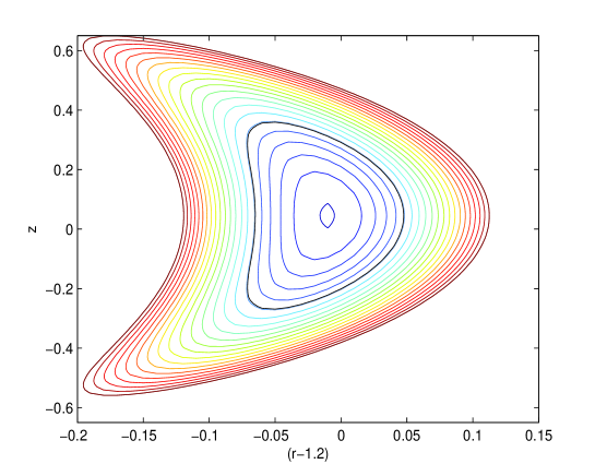
Figure 1: $u$-contours on the poloidal plane for an equilibrium of the class of solutions (10). The black-colored D-shaped curve corresponds to the boundary of a tokamak pertinent equilibrium shown separately in Fig. 2.

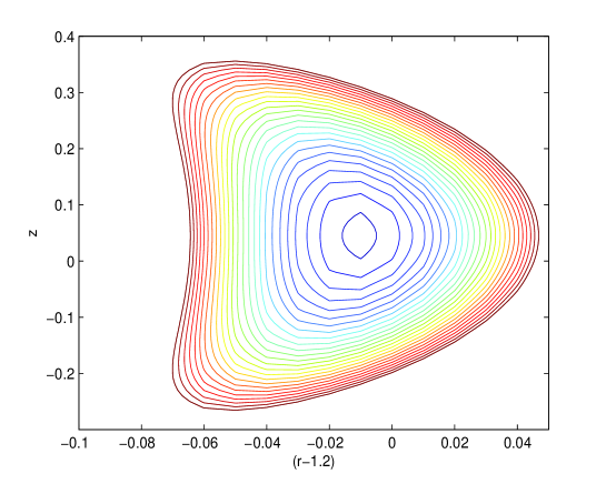
Figure 2: $u$-contours on the poloidal plane for the tokamak D-shaped equilibrium.

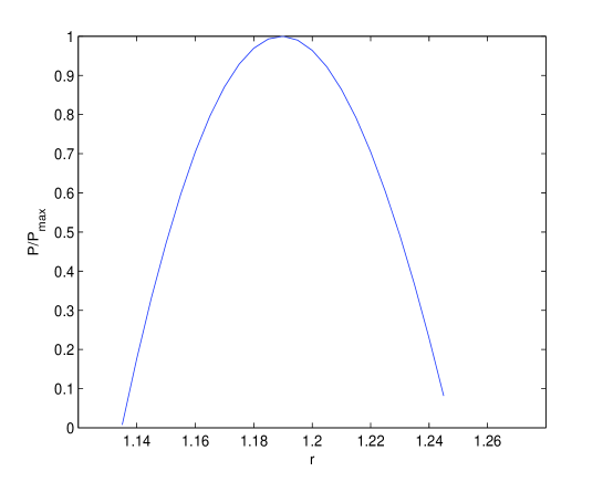
Figure 3: The pressure profile on the plane $z=0$ for the D-shaped equilibrium of Fig. 2. It vanishes on the boundary of the D-shaped equilibrium at $u_{b}=-132.543$ Wb. Here $P_{max}=0.316$ Atm.

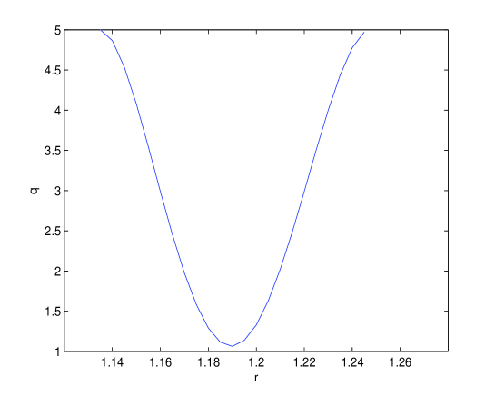
Figure 4: The safety factor for the D-shaped equilibrium of Fig. 2.

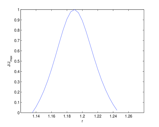
Figure 5: The current density for the D-shaped equilibrium of Fig. 2. It vanishes on the boundary of the D-shaped equilibrium. Here $J_{max}\simeq 1.7MA/m^{2}$.

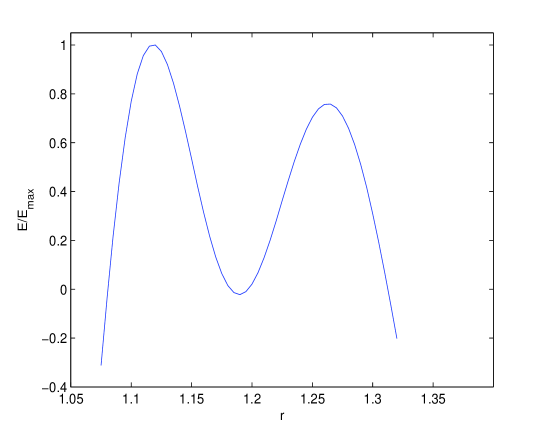
Figure 6: The electric field for the D-shaped equilibrium of Fig. 2. It vanishes on axis. Here $E_{max}=$ 1 Kv/m.

To completely construct the equilibrium we choose the Mach-function and density peaked on the magnetic axis and vanishing on the boundary as $M_{p}^{2}(u)=M_{0}^{2}(1-u^{2}/u_{b}^{2})$, $\rho=\rho_{0}(1-u^{2}/u_{b}^{2})$ respectively, where $M_{0}^{=}0.02$ and $\rho_{0}=4\times 10^{-7}$ Kg/m³. The pressure of the D-shaped equilibrium of Fig. 2, peaked on axis and vanishes on the boundary, is shown in Fig. 3. The safety factor has a typical tokamak variation monotonically increasing from the magnetic axis to the boundary, as can be seen in Fig. 4. The toroidal current density is also peaked on axis and vanishing on the boundary (Fig. 5) unlike a hollow $J_{\phi}$ profile of an equilibrium with parallel flow corresponding to the same ansatz (6) with $a_{4}=0$ constructed in kuth . This result indicates that the electric field associated with the non-parallel component of the flow, shown in Fig. 6, may play a role in determining the equilibrium characteristics.

In summary, by employing Lie and weak conditional symmetries of a GGS equation for plasmas with incompressible flow of arbitrary direction we have extended a class of nonlinear axisymmetric solutions obtained in cico2 . In particular, we constructed a D-shaped configuration with sheared electric field and typical tokamak equilibrium characteristics, i.e. pressure and toroidal current density peaked on the magnetic axis and safety factor monotonically increasing from the axis to the boundary. It would be interesting to extend the search for other relevant equilibria by potentially identifying other weak conditional symmetries following the procedure of cico1 and cico2 . Work along these lines is in progress.

Aknowledgments

This work has been carried out within the framework of the EUROfusion Consortium and has received funding from the National Programme for the Controlled Thermonuclear Fusion, Hellenic Republic. The views and opinions expressed herein do not necessarily reflect those of the European Commission.

References

- (1) P. J. Olver, Application of Lie Groups to Differential Equations (Springer Berlin, 1986).
- (2) CRC Handbook of Lie Group Analysis of Differential Equations edited by N. H. Ibragimov (CRC, Boca Raton, 1994), Vols 1-3.
- (3) G. W. Bluman and S. C. Anco, Symmetry and Integration Methods for Differential Equations (Springer, New York, 2002).
- (4) O. V. Kaptsov, Sov. Phys. JETP 71, 296 (1990).
- (5) R. L. White and R. D. Hazeltine, Phys. Plasmas 16, 123101 (2009).
- (6) G. Cicogna, F. Pegoraro and F. Ceccherini, Phys. Plasmas 17, 102506 (2010).
- (7) Y. E. Litvinenko, Phys. Plasmas 17, 074502 (2010).
- (8) R. Cimpoiasu, Phys. Plasmas 21, 042118 (2014).
- (9) H. Tasso and G. N. Throumoulopoulos, Phys. Plasmas 5, 2378 (1998).
- (10) Ch. Simintzis, G. N. Throumoulopoulos, G. Pantis and H. Tasso, Phys. Plasmas 8, 2641 (2001).
- (11) G. N. Throumoulopoulos, H. Tasso, G. Poulipoulis, J. Plasma Physics 74, 327 (2008).
- (12) G. Cicogna and F. Pegoraro, Phys. Plasmas 22, 022520 (2015).
- (13) U. Gebhardt and M. Kiessling, Phys. Fluids B 4, 1689 (1992).
- (14) T. Andreussi, P. J. Morrison, and F. Pegoraro, Phys. Plasmas 19, 052102 (2012).
- (15) Ap Kuiroukidis, and G. N. Throumoulopoulos, Plasma Phys. Control. Fusion 56 075003 (2014).