Oscillatory dynamics in complex recurrent neural networks

Abstract

Spontaneous oscillations measured by Local field potentials (LFPs), electroencephalograms and magnetoencephalograms exhibits variety of oscillations spanning frequency band ($1-100$ Hz) in animals and humans. Both instantaneous power and phase of these ongoing oscillations have commonly been observed to correlate with pre-stimulus processing in animals and humans. However, despite of numerous attempts it is not fully clear whether the same mechanisms can give rise to a range of oscillations as observed in vivo during resting state spontaneous oscillatory activity of the brain. In the current paper we show how oscillatory activity can arise out of general recurrent on-center off-surround neural network. The current work shows (a) a complex valued input to a class of biologically inspired recurrent neural networks can be shown to be mathematically equivalent to a combination of real-valued recurrent network with real-valued feed forward network, (b) such a network can give rise to oscillatory signatures. We also validate the conjecture with results of simulation of complex valued additive recurrent neural network.

1 Introduction

It has always been a standard practice to break down the brain signals obtained in electroencephalography (EEG) or magnetoencephalography (MEG) in terms of their frequency components obeying the laws of Fourier decomposition. It is even commonplace to compartmentalize the frequencies into neat bunches like $\theta$ (4-8 Hz), $\alpha$ (8-12 Hz), etc. However, the important question is whether these bands are just a matter of convenience or is there an underlying reality to the oscillatory model for the brain. Some recent work has tried to tie the oscillatory framework to underlying spiking model for neurons [2, 10]. This question can be solved only by looking at mathematical properties of neural codes.

In recent years the understanding of neural codes has provided us with insights that go beyond the concepts of rate coding and it is increasingly more commonplace to speak of temporal codes that use spike timing and phase information in order to transmit and process information reliably [12, 14, 7, 3]. However, most of these attempts are to look at neural codes after the presentation of stimulus. Recently, some studies have looked at pre-stimulius brain states in MEG and EEG based studies and have found that it is possible to predict conscious detection of stimuli based on pre-stimulus oscillatory brain activity [8, 15, 9, 5]. For instance in case of near threshold stimuli some researchers have found the pre-stimulus $\alpha$ frequency band modulation to be important [15]. These attempts have drawn a large amount of interest, but have revealed little towards a theoretical or physiological understanding of such phenomena. In the current work we have tried to start from a minimal number of assumptions regarding a neuronal assembly and tried to show how it is possible to theoretically derive such an oscillatory dynamics.

2 Methods

Conjecture 1

If a neural assembly $\mathbb{S}$ of $N$ neurons consists of both feed-forward and recurrent connections with a finite variable bound refractory period $\tau$ between the feed-forward and recurrent connections, the equilibrium solution for the assembly can be characterized by a class of oscillatory functions.

Justification

If a neural assembly comprises of $n_{1}$feed-forward neurons and $n_{2}$ recurrent neurons ($n_{1}+n_{2}\leq N)$, then the general activations of the pools of neurons will be given by

$$\mathbf{\dot{x}_{1}}=\frac{d\mathbf{x_{1}}}{dt}\}_{n_{1}}=\textrm{sgn}(\xi^{T}\xi\mathbf{x_{1}}-\theta)$$ (1)

$$\mathbf{\dot{x}_{2}}=\frac{d\mathbf{x_{2}}}{dt}\}_{n_{2}}=-\mathbf{x_{2}}+\mathbf{F}.\mathbf{x_{2}}+\eta\mathbf{I}_{\mathbf{x_{1}}}$$ (2)

where $\xi$ is the weight matrix for the feed-forward connections, $\theta$ is the threshold, $\eta$ is a scaling multiplier, $\mathbf{F}$ is the non-linear transfer function and $\mathbf{I}_{\mathbf{x_{1}}}$ is the input coming from the feed-forward networks. Now, for the network to be useful there needs to be sustained activity (provided by the recurrent network, see [11]) as well as the ability to restart the network dynamics. The latter is provided by assuming that a smoothing regularizer is provided which varies inversely with the network output [16] (to smooth the network against noisy perturbations), as well as a global decay parameter. In such a network, the overall output function $\overline{<\mathbf{x_{1}}+\mathbf{x_{2}}>}$ (average expectation value of the network output constructed in the line of mean activation in [11]), varies between 0 and $\overline{<\mathbf{x_{2}}>}+I$, where $I$ is the average normalized input to the network. This alone is sufficient to show the possibility of oscillatory solutions. However, to be more rigorous, let us look at the second order time evolution for the feed-forward and recurrent populations. From Eq. 1 we get.

$$\mathbf{\ddot{x}_{1}}=\frac{d^{2}\mathbf{x_{1}}}{dt^{2}}\}_{n_{1}}=\pm 2\delta(\xi^{T}\xi\mathbf{x_{1}}-\theta)$$ (6)

Here $\delta(x)$ is the Dirac delta function. From Eq. 2 we have,

$$d\mathbf{\dot{x}_{2}} = -d\mathbf{x_{2}}+d(\mathbf{F}.\mathbf{x_{2}})$$ (8)

$$=-d\mathbf{x_{2}}+(d\mathbf{F}).\mathbf{x_{2}}+\mathbf{F}.d\mathbf{x_{2}}$$

If $\mathbf{F}$ is a smooth transfer function then the third term in the right hand side of Eq. 8 becomes negligible. Thus we have

$$\mathbf{\ddot{x}_{2}}=-\mathbf{\dot{x}_{2}}+\mathbf{\dot{F}}.\mathbf{x_{2}}$$ (9)

$$\mathbf{\ddot{x}_{2}}=(1-\mathbf{F})\mathbf{x_{2}}+\mathbf{\dot{F}}\mathbf{x_{2}}+\mathcal{\mathcal{O}}(\mathbf{I}_{\mathbf{x_{1}}})$$ (10)

For the recurrent network, near equilibrium (here we assume absence of input because of the finite refractory period of $\tau$), the nonlinear operators $\mathbf{F}$ and $\mathbf{\dot{F}}$ become quasi-linear operators, and thus we have

$$\mathbf{\ddot{x}_{2}}=\frac{d^{2}\mathbf{x_{2}}}{dt^{2}}\}_{n_{2}}=-\parallel\mathbf{F}-(1+\mathbf{\dot{F}})\parallel\mathbf{x_{2}}$$ (11)

This has a form of simple eigenvalue problem. The network will have oscillatory solution if the operator $\parallel\mathbf{F}-(1+\mathbf{\dot{F}})\parallel$ is positive Hermitian. A suitable example is the leaky accumulator network described in [11] where the matrix representing the operator becomes real symmetric. Thus near equilibrium, considering $\mathbf{F}$ is a quasi-linear approximation $<\mathbf{x_{2}}>$, the mean state of the neural assembly near equilibrium / steady state will have a periodic solution $\xi_{n}=Ae^{i(\omega_{n}t-\theta)}$ with $\mathbf{x_{1}}$ contributing to the phase $\theta$. The full neural field dynamics $\psi(x,t)$ can be constructed along the lines of [4] with both spatial and temporal components taken into account as the following

$$\psi(x,t)=\sum\xi_{n}(t)\exp(inkx)$$ (12)

Thus the predictions from this analytical framework can be easily ported to neural mass models as well.

Corollary

An assembly of recurrent neurons with complex-valued inputs and outputs, is formally equivalent to a neural assembly of independent feed-forward and recurrent neurons.

Justification

Let us start with Cohen-Grossberg generalized networks of additive variant with a nonlinear activation function, like the network described by [11, 13, 1]. If inputs and outputs to the network are given by a vector of complex numbers $\bar{\mathbf{z}}_{\{1\times m\}}=\bar{\mathbf{x}}_{\{1\times m\}}+i\bar{\mathbf{y}}_{\{1\times m\}}$ for a network of $m$ nodes, the network dynamics is governed by

$$\frac{dz_{j}}{dt}=-z_{j}+c_{1}F(z_{j})-c_{2}\sum_{k\neq j}F(z_{k})+I_{j}+\mathrm{noise}$$ (13)

where $F(z)=z/(1+z)$. Ignoring noise for the time being, if we decompose the real and imaginary parts of 13, we have

$$\begin{split}\frac{dz_{j}}{dt}&=-z_{j}+c_{1}\frac{z_{j}+\left|z_{j}\right|^{2}}{1+\left|z_{j}\right|^{2}+2\mathrm{Re}(z_{j})}\\ &-c_{2}\sum_{k\neq j}\frac{z_{k}+\left|z_{k}\right|^{2}}{1+\left|z_{k}\right|^{2}+2\mathrm{Re}(z_{k})}+I_{j}\end{split}$$ (14)

And thus the separated real and imaginary parts yield two equations given by,

$$\begin{split}\frac{d\mathrm{Re}(z_{j})}{dt}&=-\mathrm{Re}(z_{j})+c_{1}\frac{\mathrm{Re}(z_{j})}{1+\left|z_{j}\right|^{2}+2\mathrm{Re}(z_{j})}\\ &-c_{1}\sum_{k\neq j}\frac{\mathrm{Re}(z_{k})}{1+\left|z_{k}\right|^{2}+2\mathrm{Re}(z_{k})}+\mathrm{Re}(I_{j})+\mathcal{O}(\left|z\right|^{2})\end{split}$$ (15)

$$\frac{d\mathrm{Im}(z_{j})}{dt}=\sum c^{\prime}_{jk}\mathrm{Im}(z_{k})+\mathrm{Im}(I_{j})$$ (16)

where $c^{\prime}_{jk}$ are constants. Making suitable substitutions ($x_{j}\leftarrow 2(\mathrm{Re}(z_{j})+\left|z_{j}\right|^{2}/2)$, and $y_{j}\leftarrow\mathrm{Im}(z_{j})$ ), we have

$$\frac{dx_{j}}{dt}=-x_{j}+c"_{1}F(x_{j})-c"_{2}\sum_{k\neq j}F(x_{k})+I_{j}+\textrm{constant terms}$$ (17)

$$\frac{dy_{j}}{dt}=\sum c^{\prime}_{jk}y_{k}+I^{\prime}_{j}$$ (18)

From Eq. 17 and 18 it is clear that a combination of recurrent and feedforward networks can function in a way to handle complex inputs and outputs and thus at least the reverse of Conjecture 1 is true in certain cases.

In the following section we show simulations involving additive neural networks giving rise to oscillatory dynamics under complex inputs.

3 Results

In the above, we have shown the possibility of oscillatory brain states under certain equilibrium conditions for a neural assemble consisting of both feed-forward and recurrent connections. We simulated a recurrent on-center off-surround neural network governed by the dynamical equation (complex version of the neural network used in [11])

$$\frac{dz_{i}}{dt}=-x_{i}+\alpha F(z_{i})-\beta\sum_{j=1,j\neq i}^{N}F(z_{j})+I_{i}+noise$$ (19)

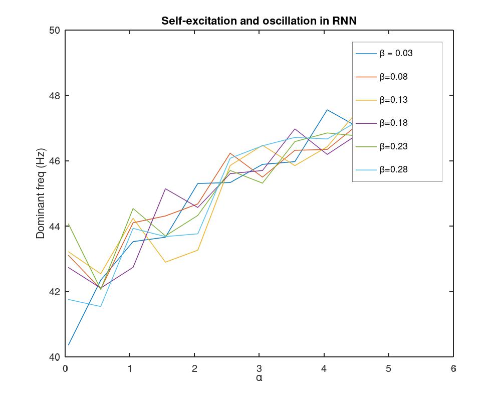
where $z_{i}$ are complex valued activations of the nodes indexed 1 to $N$ (we used 10 nodes for the simulation). All the nodes are fully connected with self-excitation $\alpha$ (we used values 0.05, 0.55, 1.05, 1.55, 2.05, 2.55, 3.05, 3.55, 4.05, 4.55, 5.05) and lateral inhibition $\beta$ (we used 0.03, 0.08, 0.13, 0.18, 0.23, 0.28). Transfer function $F$ is defined as

$$F(z)=\frac{z}{1+z}$$ (20)

$I_{i}$ is a transient complex input for 200 ms steps with values clamped at ($0.7+0.1i$).

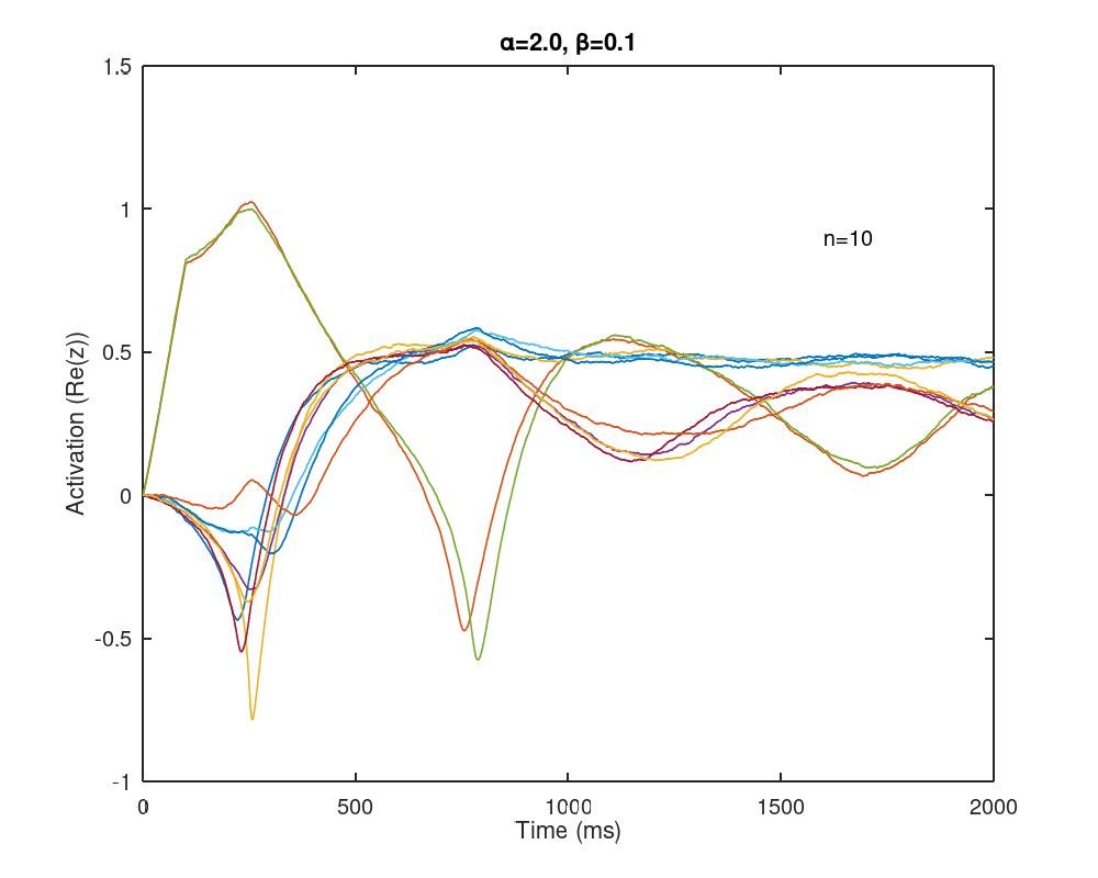
We ran the numerical simulation for total 2000 ms steps using time steps of 0.01 using Euler method. Noise was sampled from a Gaussian distribution with mean 0 and standard deviation of 0.05. Fig. 1 depicts $\mathrm{Re}(z)$ for the network for network parameters $\alpha=2.0$ and $\beta=0.1$.

Figure 1: Real values of the activation for the nodes of the network where $\alpha=2.0$ and $\beta=0.1$.

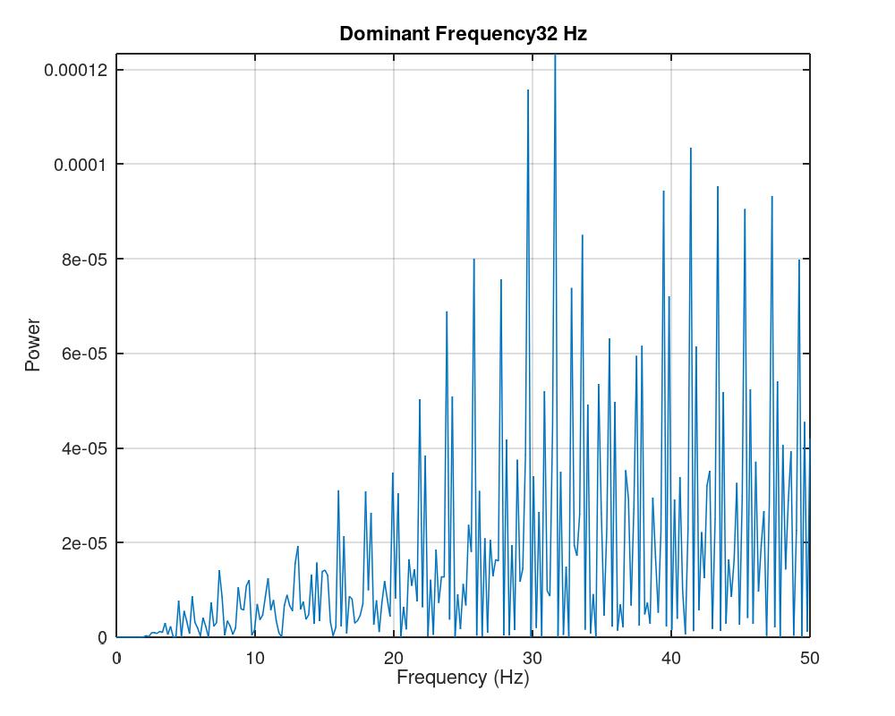
We ran time-frequency analysis on $\mathrm{Re}(z)$ and the results are shown in Fig. 2. We ran 100 simulations for each values of $\alpha$ and $\beta$ and Fig. 3 shows the average dominant frequency values for all $\alpha$ and $\beta$.

Figure 2: Frequency power analysis for $\mathrm{Re}(z)$ for the nodes of the network where $\alpha=2.0$ and $\beta=0.1$.

Figure 3: Average dominant frequency values for all the $\alpha$ and $\beta$ values in simulation.

4 Discussion

In the above, we have shown the possibility of oscillatory brain states under certain equilibrium conditions for a neural assemble consisting of both feed-forward and recurrent connections. We also showed with help of simulations (Fig. 1, 2 & 3) that simple fully connected additive recurrent neural network with complex inputs can lead to oscillatory dynamics. We saw in Fig. 3 that dominant frequency of the steady-state dynamics varies linearly with the self-excitation parameter ($\alpha$) of the network, but not with the lateral inhibition ($\beta$). In the future we intend to investigate similar dynamics for other recurrent network variants like multiplicative and self-organized maps, etc.

Appendix A Cognitive dynamics and pre-stimulus oscillations

Conjecture

If a neural assembly $\mathbb{S}$ of $N$ neurons consists of both feed-forward and recurrent connections with a finite variable bound refractory period $\tau$ between the feed-forward and recurrent connections, the pre-stimulus brain states are determined by the delay between the regions represented by the neural assemblies.

Justification

The conjecture 1 has some interesting consequences. Firstly, it allows for brain states to be defined in terms of a frequency or a distribution of frequencies. In a case of a state with a distribution of frequencies we can think of a characteristic frequency range representing the state, the characteristic frequency being the one with maximal power. The conjecture also allows us to think of the brain states as phenomenal superposition of oscillatory dynamics, allowing us to deal with problems such as stimulus related perturbations to brain states more efficiently.

The prevailing additive idea of brain states in the neuroimaging literature needs no introduction. However, we will formally spell out the bare essentials. Before a test condition appears to a subject the family of brain states or the neural assembly $\mathbb{S}$ in question ($S$) can be thought of as its resting state. In the test condition, a new perturbation comes from our experimental control ($S_{T}$). Or we can write, $S\leftarrow\bar{S}+S_{T}$.

Now if the resting state is imagined as a standing wave, then we have from Eq. 12 $\bar{S}=\sum A\mathrm{cos}(kx)\mathrm{exp}(i\omega_{0}t)$. Since resting state can be taken to be not very location specific we can write the rate of change of the state of neural assembly given by $S$, when a perturbative brain state $S_{T}$ (generally due to oncoming stimulus) interacts with the current state to be given by

$$\frac{\partial S}{\partial t}=i\alpha\mathrm{exp}(\omega_{0}t)+\frac{\partial S_{T}}{\partial t}$$ (21)

From the results of the previous section, if assume the brain states and their perturbations to have solutions of the form $Ae^{i(\omega t-\theta)}$ we can write,

$$a_{1}i\omega e^{i(\omega t-\theta)}=i\alpha e^{\omega_{0}t}+a_{2}i\omega^{\prime}e^{i(\omega^{\prime}t-\theta_{1})}$$ (22)

Here $\omega$ is the pre-stimulus brain state frequency that tries to interact with the incoming perturbation characterized by $\omega^{\prime}$. Separating the real and the imaginary parts and applying the constraint that the imaginary part must go to zero on the left and right hand side of Eq. 22

$$a_{1}\omega\cos(\omega t-\theta)=\alpha\cos(\omega_{0}t)+a_{2}\omega^{\prime}\cos(\omega^{\prime}t-\theta_{1})$$ (23)

Now considering the case $\omega\sim\omega^{\prime}$, we have from Eq. 23 (if $S$ and $S_{T}$ are in similar phase) we have for $t\rightarrow 0$,

$$(a_{1}-a_{2})\omega\cos(\omega t-\theta)=\alpha$$ (24)

Thus we have our constraint,

$$-1\leq\frac{\alpha}{(a_{1}-a_{2})\omega}\leq 1$$ (25)

Thus Eq. 25 shows that the resonant frequency of the pre-stimulus brain states in a region varies with $\alpha$. Interestingly, $\alpha$ is a spatial term dependent on the spatial connectivity as seen above. Thus the frequencies generated in the oscillatory pre-stimulus brain will depend upon the delay between the regions.

Thus there are two consequences of the analytical framework. It shows how a general oscillatory activity can be generated in the particular brain region having both feedforward and recurrent connections. Secondly it connects the general oscillatory signals in the brain that arises from connected regions to be dependent upon the delay in the network connectivity arising from spatial factors.

References

- [1] Rafal Bogacz, Marius Usher, Jiaxiang Zhang and James L. McClelland “Extending a biologically inspired model of choice: multi-alternatives, nonlinearity, and value-based multidimensional choice” In Philosophical Transactions of the Royal Society B: Biological Sciences 362, 2007, pp. 1655–16709 DOI: 10.1017/cbo9780511731525.009
- [2] G. Deco et al. “Key role of coupling, delay, and noise in resting brain fluctuations” In Proceedings of the National Academy of Sciences USA 106.25, 2009, pp. 10302–10307 DOI: 10.1073/pnas.0901831106
- [3] Jacques Gautrais and Simon Thorpe “Rate coding versus temporal order coding: a theoretical approach” In Biosystems 48, 1998, pp. 57–65 DOI: 10.1016/s0303-2647(98)00050-1
- [4] V.. Jirsa and H. Haken “Field Theory of Electromagnetic Brain Activity” In Physical Review Letters 77, 1996, pp. 960–963 DOI: 10.1103/physrevlett.77.960
- [5] J. Keil, N. Muller, N. Ihssen and N. Weisz “On the Variability of the McGurk Effect: Audiovisual Integration Depends on Prestimulus Brain States” In Cerebral Cortex 22, 2012, pp. 221–231 DOI: 10.1093/cercor/bhr125
- [6] Danilo Mandic and Jonathon Chambers “Recurrent neural networks for prediction: learning algorithms, architectures and stability” Wiley, 2001
- [7] Timothée Masquelier “Relative spike time coding and STDP-based orientation selectivity in the early visual system in natural continuous and saccadic vision: a computational model” In Journal of Computational Neuroscience 32, 2012, pp. 425–441 DOI: 10.1007/s10827-011-0361-9
- [8] K.. Mathewson et al. “To See or Not to See: Prestimulus \textalpha Phase Predicts Visual Awareness” In Journal of Neuroscience 29, 2009, pp. 2725–2732 DOI: 10.1523/jneurosci.3963-08.2009
- [9] Elisabeth S. May et al. “Pre- and post-stimulus alpha activity shows differential modulation with spatial attention during the processing of pain” In Neuroimage 62, 2012, pp. 1965–1974 DOI: 10.1016/j.neuroimage.2012.05.071
- [10] Tristan T. Nakagawa et al. “How delays matter in an oscillatory whole-brain spiking-neuron network model for MEG alpha-rhythms at rest” In Neuroimage 87, 2014, pp. 383–394 DOI: 10.1016/j.neuroimage.2013.11.009
- [11] Rakesh Sengupta, Bapi Raju Surampudi and David Melcher “A visual sense of number emerges from the dynamics of a recurrent on-center off-surround neural network” In Brain Research 1582, 2014, pp. 114–224
- [12] Garrett B. Stanley “Reading and writing the neural code” In Nature Neuroscience 16, 2013, pp. 259–263 DOI: 10.1038/nn.3330
- [13] Marius Usher and Jonathan D Cohen “Short term memory and selection processes in a frontal-lobe model” In Connectionist models in Cognitive Neuroscience Springer, 1999, pp. 78–91
- [14] R. van Rullen and Simon J. Thorpe “Rate Coding Versus Temporal Order Coding: What the Retinal Ganglion Cells Tell the Visual Cortex” In Neural Computation 13, 2001, pp. 1255–1283 DOI: 10.1162/08997660152002852
- [15] N. Weisz et al. “Prestimulus oscillatory power and connectivity patterns predispose conscious somatosensory perception” In Proceedings of the National Academy of Sciences, USA 111, 2014, pp. E417–E425 DOI: 10.1073/pnas.1317267111
- [16] Lizhong Wu and John Moody “A Smoothing Regularizer for Feedforward and Recurrent Neural Networks” In Neural Computation 8, 1996, pp. 461–489 DOI: 10.1162/neco.1996.8.3.461