France new regions planning? Better order or more disorder ?

Abstract

This paper grounds the critique of the ’reduction of regions in a country’ not only in its geographical and social context but also in its entropic space. The various recent plans leading to the reduction of the number of regions in metropolitan France are discussed, based on the mere distribution in the number of cities in the plans and analyzed according to various distribution laws. Each case, except the present distribution with 22 regions, on the mainland, does not seem to fit presently used theoretical models. Beside, the number of inhabitants is examined in each plan. The same conclusion holds. Therefore a theoretical argument based on entropy considerations is proposed, thereby pointing to whether more order or less disorder is the key question, - discounting political considerations.

Keywords: France; regional planning; number of inhabitants; number of cities; entropy considerations

I Introduction

According to United Nations Department of Economic and Social Affairs reports ONU_2009 , the majority of the world population resides in urban areas for the first time in human history. Municipalities are emerging as key sites of social experimentation and problems in the 21st century Bettencourt and West_2010 ; Glaeser_2011 ; Grabar_2013 ; Katz and Bradley_2013 . In several countries, the number of municipalities were or will be regrouped to form larger entities, ”cities”, supposedly more manageable in various ways. Obviously, the number of municipalities will be smaller. There is a tendency to see the number of municipalities as a kind of universal, rational and officially depoliticised process, since bearing on numbers rather than population size or wealth, in contrast to and in order to avoid claims of gerrymandering Martis_2008 . Both geographers and planners have been using increasingly sophisticated quantitative and computational methods to explain, suggest or even recommend the number reduction Cox and Mair_1988 ; McCann and Ward_2010 . The point is not discuss such hypotheses nor ”reasonings” which are, as usually admitted, quite debatable, and surely time dependent. Interestingly, another type of number reductionism process occurs at the next administrative level, i.e. the reduction in the number of departments, provinces, regions, depending on the country structure, e.g. as can be illustrated through European statistics NUTS_2013 .

Consider France (FR), as a timely example. The country is made of 27 regions and 101 departments: 22 regions constitute the ”Metropolitan France”, while 5 regions, which are also departments, make the Overseas Territories, called DOM-TOM. (DOM: Départements d’Outre-Mer, or overseas departments; TOM = ”Territoires d’Outre-Mer”, or overseas territories. Both are often grouped as DOM-TOM.) Several proposals have been presented about regrouping the departments into a smaller number of new regions, - supposedly for various administrative and economic reasons, mainly, i.e. to reduce administrative spending, as it has been claimed, but also surely according to some public opinion, to concentrate political power. Some considered regrouping, from 22 to 15, $\dots$, down to 11 regions, envisaged at various recent times, is briefly recalled here below in Sect. II. On Wednesday Dec. 17, 2014, the French Parliament voted to reduce the number of regions to 13 with still some possibility for departments to negotiate their regional membership later. (The reform will be in effect in 2016). There were and still are many manifestations of anger concerning the new regional distribution and content, for diverse reasons. This anger is not of real concern for this paper. Nevertheless, an objective data analysis might shine some light on the process.

The number of departments will remain unchanged. The number of elected councilors will also remain the same. Of course, political power might be modified according to the assembly member political affiliations. The criterion has not been mentioned, although in a related affair, i.e. the regrouping of municipalities in Belgium, to redistribute local power was the main criterion. Nevertheless, let us neglect such a point of view at this level.

Thus, neglecting political constraints, it seems of interest to observe whether the regrouping of regions in FR obeys theoretical laws on the grouping of settlements in an area, according to Gibrat Gibrat or or Yule yule1922 models and subsequent laws. These are not universally obeyed, but they are based on scientific reasoning tied to common sense BGNEGNKVZID . In that spirit, it is fair to mention a broader study of the parametric description of city size distributions (in four European countries: France, Germany, Italy and Spain) by Puente-Ajovin and Ramos Puente-Ajovin and Ramos_2015 through several parametric models. The results are quite coherent. Therefore, for our endeavor, there is no need here to investigate the flurry of models as discussed by Puente-Ajovin and Ramos Puente-Ajovin and Ramos_2015 .

To test those models or rules, the standard way of presenting the administrative content of regions is through the rank-size relationship BGNEGNKVZID ; GabaixIoannides04 ; Brakmanetal99 ; ZDMA , i.e. a display of the list of regions ranked from $r=1$ to its maximum value $r_{M}$, i.e. the number of regions, $N_{r}$. The ranking is based on the number of municipalities in each region $N_{c,r}$, given in decreasing order. For example, Midi-Pyrénées is the French region having the largest number of municipalities (3020), in recent times. The present list is given in Table 3.

The FR number of municipalities , more than 36 000, has been varying almost monthly, although not drastically. Thus, to take such a number evolution over the last few years in the following analysis is not mandatory: the Dec. 2014 law on region regrouping is based indeed on a rather so called stable situation. Thus, the number of municipalities which is considered is that available in Jan. 2014, when the ”final” discussion on the number of regions and their extent last line of discussion started in the French National Assembly. Nevertheless, for convincing the reader, the data on the number of municipalities distribution is also given in Table 3 for the Jan. 2012 time.

It will be of common sense interest to compare considerations on municipalities with the number of inhabitants, which is known in contrast to be a very fluctuating quantity. It was above 63 millions for the metropolitan FR in Jan. 2014 according to INSEE official data INSEEdataNib . Thus, beside the (distribution of the) number of municipalities , the (distribution of the) number of inhabitants is examined in each case here below, within the same statistical framework, along a statistical distribution pertaining to the matter, in Sect. III. N.B. The 6 municipalities without inhabitants in metropolitan FR have been taken all into account.

Thus, region ranking will be found through their $N_{i,r}$ content. It should be understood at once that the ranking $N_{c,r}$ and $N_{i,r}$, are a priori not correlated. In fact, only the two highest ranked regions, Limousin and Corse, maintain their identical rank (21 and 22) in both the number of municipalities and the number of inhabitants.

It is re-stressed that the paper emphasis is on the region number and city number distribution content as a basis for estimating the interest of the proposed plans on a purely numerical basis. Two warnings are still needed at this point. (i) Some analysis difficulty is due to Corse. The island actually forms a region, - with 360 municipalities all together. This number of municipalities is clearly an outlier from a statistical point of view. However, it will be seen that political plans have sometimes imagined that Corse could be merged with some other region from Southern France, - see Sect.II. Thus, for coherence, Corse, although an outlier, has been kept as such in the following data analysis, a priori knowing as a consequence that it would induce a larger error bar on the fit parameters than otherwise. (ii) The DOM-TOM regions or departments are not included much in the following discussion since the discussed region regrouping is irrelevant in their case.

A discussion of the fit features is found in Sect. IV. It will appear that the various intended regroupings are not theoretically highly convincing, to say the least. A suggestion for a complementary approach will be emphasized with a ”thermodynamic/information entropy” argument in Sect.V. A conclusion is found in Sect.VI.

Moreover, for some ”completeness”, some brief analysis of the ranking relationship of departments $only$ according to their number of municipalities is presented in an Appendix. In so doing, the emphasis on outlier effects, for this case, is quite well seen.

II Brief review of a few regrouping plans in a chronological way

The reduction of the metropolitan regions is not a new idea. In 2009, a Committee of reform of the local government agencies, chaired by the former Prime Minister E. Balladur, had one of its proposals, hereby called B15, recommending to reduce the number of regions to 15 areas: Alsace-Lorraine, Auvergne-Limousin, Bourgogne-Franche Comté, Bretagne, Champagne, Corse, Ile de France, Languedoc-Roussillon, Midi-Pyrénées, Nord-Pas de Calais, Normandie, Poitou-Aquitaine, Provence-Rhône-Alpes, Val de Loire-Centre. N.B. Fusions of the areas are best seen when reading Table 3. Notice that the french names are kept. A few names could be used either in english or in french: Burgundy$\leftrightarrow$ Bourgogne, Brittany $\leftrightarrow$ Bretagne, Corsica $\leftrightarrow$ Corse, Normandy $\leftrightarrow$ Normandie, Center $\leftrightarrow$ Centre.

In January 2014, President F. Hollande wished to divide by 2 the number of regions, leading to a map hereby called M11. It can be imagined which would be the list of these 11 new areas: Alsace-Lorraine, Aquitaine, Auvergne-Rhône, Bourgogne-Franche Comté, Bretagne, Grand Paris, Languedoc-Roussillon, Nord-Pas de Calais, Normandie, Provence-Alpes-Côte d’Azur-Corse, Val de Loire. N.B. This plan intends to merge Corse with the Provence-Alpes-Côte d’Azur region.

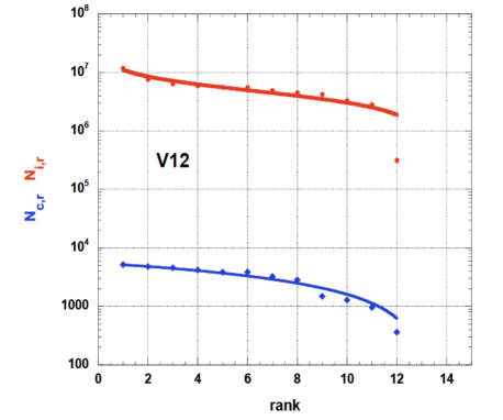
However, the Prime Minister M. Valls proposed a territorial reform on Tuesday, April 8, 2014 based on 12 metropolitan regions, called V12 here below: Aquitaine-Poitou-Limousin, Artois-Picardie, Bourgogne-Franche Comté, Bretagne, Champagne-Alsace-Lorraine-Ardennes, Corse, Ile de France, Midi-Pyrénées-Languedoc-Roussillon, Normandie, Provence-Alpes-Côte d’Azur, Rhône-Alpes-Auvergne, Val de Loire.

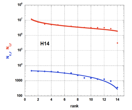
Next on Monday, June 2, 2014, F. Hollande proposed a map with 14 new areas, called H14 here below, i.e. Alsace-Lorraine, Aquitaine, Auvergne-Rhône-Alpes, Bourgogne-Franche Comté, Bretagne, Corse, Ile de France, Midi-Pyrénées-Languedoc-Roussillon, Nord-Pas de Calais-Champagne, Normandie, Pays de la Loire, Picardie-Champagne-Ardennes, Poitou-Charente-Limousin-Centre, Provence–Alpes-Côte d’Azur.

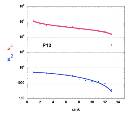
In fine, the national Assembly adopted on Friday, July 18, 2014 a map of France with 13 metropolitan regions. Due to much discussion with the Senate and local authorities, another 13 new region map of France was adopted at the national Assembly, in the night of Wednesday 19th November 2014, but finally on Wednesday Dec. 17, 2014, the ”final” map was approved, to be in effect on the horizon 2016. The new map strictly merges regions, in contrast to other plans which allowed changes in present region borders. The new regions are: (i) Poitou-Charentes, the Limousin and Aquitaine; (ii) Nord-Pas-de-Calais and Picardy; (iii) Champagne-Ardenne, Alsace and Lorraine; (iv) Auvergne and Rhône-Alpes; (v) Bourgogne and Franche-Comté; (vi) Languedoc-Roussillon and Midi-Pyrénées; (vii) High-Normandie and Lower Normandie. Six areas remain unchanged: Brittany, Corse, Ile-de-France, Centre, Pays de la Loire, and Provence-Alpes-Côte d’Azur. This will be called the P13 plan.

III Data analysis

,

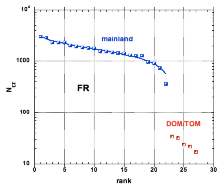
The present (Jan. 2014) number of municipalities $N_{c,r}$ in each of the 27 regions is given in Table 3, thus including the DOM-TOM for completeness. The rank-size relationship is displayed in Fig. 1. A fit is proposed through a reasonable distribution function describing a rank-size rule with 3 parameters

$$y(r)=A\;m_{1}\;r^{-m_{2}}\;(N-r+1)^{m_{3}},$$ (1)

where $A$ is an order of magnitude amplitude, a priori imposed and adapted to the data, without loss of generality, for smoother convergence of the non-linear fit process in finding the $m_{i}$ parameters in a similar order of magnitude range, and $N$ is the number of regions, of course ranked, in decreasing order of magnitude of the relevant variable, $r=1,\dots,r_{M}$, i.e. the maximum number of regions, $N_{r}$. The function has a Beta-Euler function type AbraSteg ; GradRyz which has been shown to be useful under the form

$$\kappa_{3}\;\frac{(N\;r)^{-\gamma}}{(N-r+1)^{-\xi}},$$ (2)

in other related contexts RRPh49.97.3popescu ; Glottom6.03.83popescu ; JoI1.07.155Mansilla ; JQL18.11.274Voloshynovska ; MAJAQM ; MALavPRE . It can be shown that it is related to a power law with exponential cut-off, the so called the Yule-Simon distribution Pwco3

$$y(r)=d\;r^{-\alpha}\;e^{-\lambda r},$$ (3)

which is often used in city size distribution studies. However, the latter distribution assumes that the number of elements to be ranked can extend to infinity, while Eq.(1) emphasizes a finite size limit in ranking the data. In Fig. 1), the data seems well represented by Eq.(1), when the 5 (DOM-TOM) outliers are neglected.

For completeness, a summary of the statistical characteristics for the number distribution of municipalities ($N_{c}$), in the metropolitan, including Corse, regions ($N_{c,r}$) is given in Table 4. Observe that the number of municipalities distributions correspond to negative skewness and negative kurtosis. As expected,the ratio $\mu/\sigma$ is weakly varying, allowing us for some possible inconsistency through the INSEE data tables. The same holds true the asymmetry of the distributions whatever definition of skewness is used.

IV Result discussion

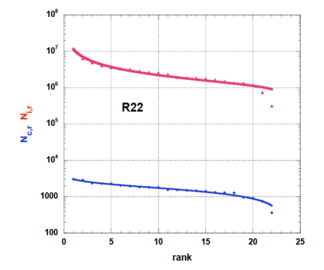
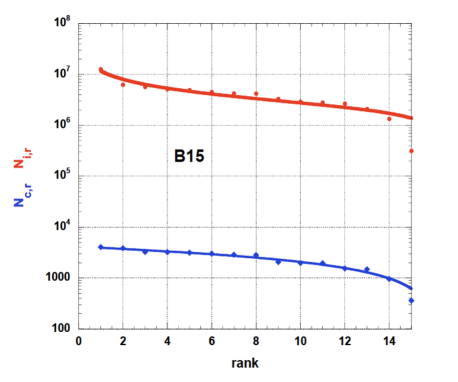
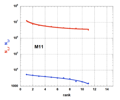
Let the main attention be focussed on the region reduction number plans for metropolitan FR. Consider the various $N_{c,r}$, and also the various possible number of inhabitants $N_{i,r}$ within each plan. The $N_{c,r}$ data of interest for continental FR is compared to the behavior of the corresponding $N_{i,r}$ data for the present 22 regions on Fig. 2. The successive figures, Fig. 3, Fig. 4, Fig. 5, Fig. 6, Fig. 7 display the corresponding data in the various cases, according to the mentioned chronology of the successive plans, presented in Sect. II. The fit parameters are given in Table 1 with the corresponding regression coefficient. The latter spans a short interval [0.962; 0.984] for the $N_{c,r}$ plans, but a slightly larger one [0.931; 0.983] for $N_{i,r}$.

It is observed from Table 1 that the best fits do not always correspond to the expected range $m_{2}>0$ and $m_{3}>0$. For $N_{c,r}$, only the present administrative distribution, R22, or the B15 plan, have both $m_{2}$ and $m_{3}$ exponents positive. In contrast, all, except M11, have both exponents positive in the $N_{i,r}$ cases. In the M11 case, one reason beside these features, might be the small number of data points, - even though one often expects a greater fit precision in such a case. In fact, the M11 plan has $quasi$ the best $R^{2}$. Nevertheless, the $N_{i,r}$ data for the M11 case markedly has no sharp decay at high rank, - since the Corse data point is missing, because the island is merged with another region in M11. Interestingly, this effect ($m_{3}\sim 0$) indicates a more equal number distribution in population between the 11 regions in this plan, except for the highly populated region ($m_{3}\neq m_{2}$).

Notice that the mid range slope, i.e. $-(m_{2}+m_{3})\;(r_{M}/2)^{(m_{3}-m_{2}-1})$, for the fit function is an indication of the $non-equality$ distribution. It is easy to derive that this slope can be = 0, i.e. $m_{3}=-m_{2}$, at $r/(r_{M}+1)=m_{2}/(m_{2}-m_{3})$, whence requesting $m_{3}>0>m_{2}$, for such an ”equality condition” case. Such cases do not exist, as can be deduced from Table 1. In contrast, the largest inequality corresponds to the largest sum $m_{2}+m_{3}$. Interestingly, - from a political view point discussion, the largest slopes occur for the new P13 in the case of $N_{c,r}$, but for the present R22 case for $N_{i,r}$. Thus, the most recent plans do not appear quite convincing from both city and population number distribution points of view.

Thus, at this investigation level, it can be concluded that the present R22 case is quite fine from a theory of settlements point of view. The next best is B15. However, these considerations admit an inequality in distributions,- which might be contrary to criteria of equality (recall the motto of the French Republic!). One counter-argument might be based on the point that the discussion does not pertain to equal maximum size systems, thus compares different systems. A more ”universal” view point should be taken! To investigate this argument, a probability framework seems pertinent, as discussed in Sect. V.

V Entropy connexion

One can consider to have access to a sort of ”probability” for finding a certain ”state” (size occurrence) at a certain rank, through

$$p(r)=\frac{N(r)}{\sum_{1}^{r_{M}}N(r)}\;\sim\;\frac{y(r)}{\sum_{1}^{r_{M}}y(r)}$$ (4)

where $N(r)$ stands for $N_{c,r}$ or $N_{i,r}$.

From Eq.(4), one can obtain something which looks like the Theil index Theil in economy or the Shannon entropy shannon in information theory, $S\equiv-\sum_{1}^{r_{M}}p(r)\;ln(p(r))$. It has to be compared to the maximum disorder number, i.e. $ln(N)$. Whence we define the relative distance to the maximum entropy as

$$d=1-\frac{S}{ln(N)}\;.$$ (5)

A small $d$ value would indicate a state of full disorder (or ”equal order”). Recall that non-equilibrium systems are those with growth (… or decay !) potential, i.e. those susceptible of evolution. Recall also that the notion of entropy maximization ($d\rightarrow 0$) of human systems is different from the concept of entropy increase in thermodynamics.

Values of interest, $d_{c,r}$ or $d_{i,r}$, in obvious notations, are reported in Table 2. First of all, a good agreement is found between the $N_{c,r}$ and $N_{i,r}$ cases, i.e. $d_{c,r}$ and $d_{i,r}$ smoothly decreases and increases respectively, as a function of $N_{r}$, accepting standard error bars, with the notable exception for the M11 plan $d_{c,r}$ which has a very small value, $\sim$ that of the present R22. Notice that the present R22 map is that with the closest distances to 0. The two smallest values occur for the M11 plan, thus suggesting that it is not drastically different from the R22, but still better from an entropic point of view. The new P13 plan has, from this entropic point of view, very similar $d_{c,r}$ and $d_{i,r}$ values, but they are not small. In fact, it has the largest $d_{c,r}$, indicating the most drastic changes with respect to the present time, from a city number distribution point of view.

VI Conclusions

Several questions were raised in the introduction,due to the multiple plans which have been proposed in order to reduce the number of regions in metropolitan France. One aim was to develop an objective analysis of the plans. Therefore, this paper provides a statistical analysis based on two numerical criteria: (i) the distribution of municipalities between France regions, and (ii) that of populations, according to those various plans proposed in recent times. These are standard variables in settlement analyses, because they rely on rather reliable numbers. It has been found that several plans weakly obeyed classical settlement models through their respective rank-size relationships. However, several cases are intriguing, in not fulfilling theoretical behaviors. Considering an entropy (disorder $vs.$ order) criterion would seem to avoid a contempt argument about this scientific approach. From such an analysis point of view, it seems that the city number or population number give opposite optimization suggestions. In fact, it is concluded that the M11 plan, based on the most simple reduction plan, seems the best for both criteria. The future P13 plan, on the contrary, seems in this respect far from respecting the second term in the motto of the French Republic (Liberté, Egalité, Fraternité).

Next, the (fundamental ?) question is of philosophical nature: is disorder better or worse than order? Often, order is claimed to be more equalitarian. However, it is known that disorder is the source of growth, - quasi all systems of interest are non-equilibrium systems. Therefore, the ”state of disorder” is a criterion to be further examined. It would be interestingly monitored for future data mining.

However, the evolution of a non-equilibrium systems, like a country state, is surely far from being described in terms of a simple set of differential equations, - for a few variables. Furthermore, a long term growth or decay evolution is quasi unpredictable, - the more so since the so called initial conditions are far from being precise. Moreover, there is no doubt that an objective set of criteria has a weak weight with respect to short term political interests, - even hidden. It seems a little bit strange also that economic considerations have not been given much weight in any plan. One can admit that this would lead to never ending debates.

In fine, notice that the final voted plan refers to the merging of regions, without questioning whether a re-distribution of departments across previous region borders, or any gerrymandering, could lead to an optimization in searching for the solution in the reduction of the number of regions problem. Note that this will be possible up to 2019, but within a very strict political scenario demanding several consensus with a 3/5 majority.

Acknowledgements This work has been performed in the framework of COST Action IS1104 ”The EU in the new economic complex geography: models, tools and policy evaluation”. Moreover, this paper is part of scientific activities in COST Action TD1210 ’Analyzing the dynamics of information and knowledge landscapes’.

VII Appendix. Department analysis

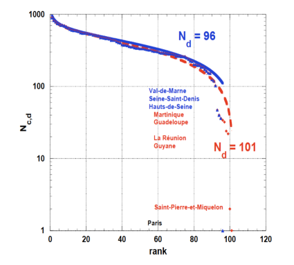
For completeness, the number distribution $N_{c,d}$ of municipalities in the FR departments can be discussed within the main text framework. Notice that ranking this data is more sensitive to the merging or creation of municipalities , since the numbers are smaller than in the region cases. E.g., the department having the greatest number of municipalities , 895, is Pas-de-Calais, among the 101 departments. In contrast, another example: Paris Department is ranked 101, - in fact, this department contains only one city, the capital of France, but belongs to the region Ile-de-France which has about 1281 municipalities . Observe that Paris ranking changes from 101 to 96 under a DOM-TOM ”elimination process”. The Paris department is clearly an outlier. See some characteristics of the distributions in Table 4.

For the demonstration, consider a semi-log plot of the number, $N_{c,d}$, of municipalities in the (metropolitan) 96 and (all) 101 FR departments ranked by decreasing order of ”importance” on Fig. 8. Interestingly, the behavior is similar to the $N_{c,r}$ cases. However, the occurrence of outliers cannot be debated. They lead to very different fit parameter values. The best 3-parameter function fit values for $N_{c,d}$ are found in Table 5.

The DOM/TOM effect is greatly emphasized, pointing to a huge disparity between the mainland and the territorial communities. Fig. 8 allows to emphasize the (visually and numerically annoying) contribution from outliers in such fits and analyses.

Figure 1: Semi-log plot of the number, $N_{c,r}$, of municipalities in the 27 FR regions ranked by decreasing order of ”importance”: blue half filled squares are for the metropolitan area; red half filled squares for the DOM-TOM. The best 3-parameter function, Eq. (1), fit is shown for the metropolitan area only ($R^{2}$= 0.978), but including Corse; the DOM-TOM have to be considered as outliers.

Figure 2: Semi-log plot of the number, $N_{c,r}$, of municipalities (blue diamonds) and $N_{i,r}$, of inhabitants (red triangles), in the 22 FR mainland regions ranked by decreasing order of importance for the R22 plan. The best 3-parameter function, Eq. (1), fit is shown for values and regression coefficient found in Table 1.

Figure 3: Semi-log plot of the number, $N_{c,r}$, of municipalities (blue diamonds) and $N_{i,r}$, of inhabitants (red triangles), in the 22 FR mainland regions ranked by decreasing order of importance for the B15 plan. The best 3-parameter function, Eq. (1), fit is shown for values and regression coefficient found in Table 1.

Figure 4: Semi-log plot of the number, $N_{c,r}$, of municipalities (blue diamonds) and $N_{i,r}$, of inhabitants (red triangles), in the 22 FR mainland regions ranked by decreasing order of importance for the M11 plan. The best 3-parameter function, Eq. (1), fit is shown for values and regression coefficient found in Table 1.

Figure 5: Semi-log plot of the number, $N_{c,r}$, of municipalities (blue diamonds) and $N_{i,r}$, of inhabitants (red triangles), in the 22 FR mainland regions ranked by decreasing order of importance for the H14 plan. The best 3-parameter function, Eq. (1), fit is shown for values and regression coefficient found in Table 1.

Figure 6: Semi-log plot of the number, $N_{c,r}$, of municipalities (blue diamonds) and $N_{i,r}$, of inhabitants (red triangles), in the 22 FR mainland regions ranked by decreasing order of importance for the V12 plan. The best 3-parameter function, Eq. (1), fit is shown for values and regression coefficient found in Table 1.

Figure 7: Semi-log plot of the number, $N_{c,r}$, of municipalities (blue diamonds) and $N_{i,r}$, of inhabitants (red triangles), in the 22 FR mainland regions ranked by decreasing order of importance for the P13 plan. The best 3-parameter function, Eq. (1), fit is shown for values and regression coefficient found in Table 1.

Figure 8: Semi-log plot of the relationship between the number, $N_{c,d}$, of municipalities in the 101 FR departments (red diamonds) ranked by decreasing order of ”importance” and in the 96 metropolitan departments (blue triangles); the best 3-parameter function fits values, Eq. (1), are shown. N.B. Paris changes rank, from 101 to 96; best 3-parameter fit values are found in Table 5 .

$N_{c,r}$	R22	B15	H14	P13	V12	M11
$Am_{1}$	915$\pm$120	638$\pm$148	211$\pm$ 91	216$\pm$114	601$\pm$241	1774$\pm$270
$m_{2}$	0.155$\pm$0.081	0.012$\pm$0.042	-0.101$\pm$0.068	-0.099$\pm$0.085	-0.015$\pm$0.077	0.108$\pm$0.036
$m_{3}$	0.390$\pm$0.038	0.674$\pm$0.078	1.162$\pm$0.153	1.227$\pm$0.195	0.864$\pm$0.151	0.458$\pm$0.058
R2	0.980	0.973	0.968	0.962	0.965	0.984
$N_{i,r}$	R22	B15	H14	P13	V12	M11
$Am_{1}/10^{6}$	7.36$\pm$1.97	5.66$\pm$2.81	7.4$\pm$2.0	4.2$\pm$1.8	43$\pm$1.9	13.96$\pm$2.2
$m_{2}$	0.678$\pm$0.034	0.521$\pm$0.083	0.510$\pm$0.070	0.382$\pm$0.080	0.334$\pm$0.092	0.554$\pm$0.042
$m_{3}$	0.141$\pm$0.084	0.269$\pm$0.175	0.168$\pm$0.131	0.385$\pm$0.157	0.379$\pm$0.169	-0.053$\pm$0.063
R2	0.983	0.936	0.948	0.947	0.931	0.981

Table 1: Parameter values allowing with Eq.(1) nice fits, as indicated by the regression coefficient R² values.

$N_{c,r}$	R22	B15	H14	P13	V12	M11
$ln(N_{r})$	3.0910	2.7081	2.6391	2.5649	2.4849	2.3979
$-\sum p\;ln(p)$	3.0126	2.6056	2.4809	2.3871	2.3260	2.3334
$d_{c,r}$	0.0254	0.0378	0.0599	0.0693	0.0639	0.0269
$N_{i,r}$	R22	B15	H14	P13	V12	M11
$ln(N_{r})$	3.0910	2.7081	2.6391	2.5649	2.4849	2.3979
$-\sum p\;ln(p)$	2.8284	2.5128	2.4837	2.4038	2.3419	2.3178
$d_{i,r}$	0.0850	0.0721	0.0589	0.0628	0.0575	0.0334

Table 2: Relative distance ($d_{c,r}$ and $d_{i,r}$) values, Eq.(5), to full disorder

$r$	Region name	$N_{c,r}$	$N_{d,r}$	$N_{c,r}$
		Jan. 2012		Jan. 2014
1	Midi-Pyrénées	3020	8	3020
2	Rhône-Alpes	2879	8	2874
3	Lorraine	2339	4	2338
4	Aquitaine	2296	5	2296
5	Picardie	2291	3	2291
6	Bourgogne	2046	4	2046
7	Champagne-Ardenne	1954	4	1953
8	Centre	1841	6	1841
9	Basse-Normandie	1812	3	1812
10	Franche-Comté	1785	4	1785
11	Nord-Pas-de-Calais	1545	2	1545
12	Languedoc-Roussillon	1545	5	1545
13	Pays de la Loire	1502	5	1496
14	Poitou-Charentes	1462	4	1460
15	Haute-Normandie	1419	2	1420
16	Auvergne	1310	4	1310
17	Île-de-France	1281	8	1281
18	Bretagne	1270	4	1270
19	Provence-Alpes-Côte d’Azur	963	6	958
20	Alsace	904	2	904
21	Limousin	747	3	747
22	Corse	360	2	360
	SUBTOTAL	36 571	96	36 552
23	Martinique	34	1	34
24	Guadeloupe	32	1	32
25	La Réunion	24	1	24
26	Guyane	22	1	22
27	Mayotte	17	1	17
	TOTAL	36 700	101	36 681

Table 3: Number $N_{c}$ of municipalities and of departments ($N_{d}$), in the (22 Mainland and Corse + 5 DOM-TOM) France regions, on Jan. 01, 2012 and 2014.

	$N_{c,r}$		$N_{c,r}$		$N_{c,d}$
	Jan.01, 2012		Jan.01, 2014		Jan.01, 2014
min	17	360	17	360	1 (**)	1 (**)
Max	3020	3020	3020	3020	895	895
$N_{c}$	36 700	36 571	36 681	36 552	36 681	3 652
$N_{r}$ or $N_{d}$	27	22	27	22	101	96
Mean ($\mu$)	1359.3	1662.3	1358.6	1661.5	363.18	380.75
Median ($m$)	1462	1545	1460	1545	332	339.50
RMS	1608.4	1781.8	1607.6	1780.9	413.32	423.91
Std Dev ($\sigma$)	876.30	656.61	875.94	656.44	198.31	187.33
Std Err	168.64	139.99	168.57	139.95	19.732	19.119
Skewness	-0.1017	0.2179	-0.1018	0.2167	0.3331	0.4416
Kurtosis	-0.7728	-0.2192	-0.7745	-0.2232	-0.2857	-0.1904
$\mu/\sigma$	1.5512	2.5316	1.5510	2.5311	1.8314	2.0325
$3(\mu-m)/\sigma$	-0.3516	0.5359	-0.3473	0.5324	0.4717	0.6606

Table 4: Summary of statistical characteristics for the number distribution of municipalities ($N_{c}$) in the various regions ($N_{c,r}$) or departments ($N_{c,d}$) in FR on different years. (**) N.B. Paris forms a department with only 1 city, itself.

	$N_{c,d}$	$N_{c,r}$	$N_{c,d}$	$N_{c,r}$
	$whole$ FR		FRmetrop
$A\;m_{1}$	446.4	111.0	848.0	916.1
$m_{2}$	0.131	0.048	0.148	0.155
$m_{3}$	0.654	0.991	0.525	0.389
$R^{2}$	0.989	0.955	0.990	0.978

Table 5: Best fit parameter values (top) in Eq. (1) for the $N_{c,d}$ data, distinguishing 101 or 96 departments; see Fig.8; some $N_{c,r}$ data fit values are repeated for ease.

References

- (1)
- (2) Bettencourt, L.; West, G. A unified theory of urban living. Nature 2010, 467, 912–913.
- (3) Glaeser, E.L. Triumph of the City: How Our Greatest Invention Makes Us Richer, Smarter, Greener, Healthier, and Happier. New York: Penguin Press 2011.
- (4) Grabar, H. (2013) Municipalities will save us! Salon, 31 July. Available online at: [Accessed 5 January 2015].
- (5) Katz, B.; Bradley, J. The Metropolitan Revolution: How municipalities and Metros Are Fixing Our Broken Politics and Fragile Economy. Washington, DC: Brookings Institution Press 2013.
- (6) Martis, K.C. The Original Gerrymander, Political Geography 2008, 27, 833-839.
- (7) Cox, K. R.; Mair, A. Locality and community in the politics of local economic development, Annals of the Association of American Geographers 1988, 78: 307-325.
- (8) McCann, E.; Ward, K. Relationality/territoriality: toward a conceptualization of municipalities in the world, Geoforum 2010, 41, 175-184.
- (9)
- (10) Gibrat, R. Les inégalités économiques: Applications aux inégalités des richesses, à la concentration des entreprises, aux populations des villes, aux statistiques des familles, etc., d’une loi nouvelle, la loi de l’effet proportionnel. Sirey, Paris, 1931.
- (11) Yule, G.U. A Mathematical Theory of Evolution, based on the Conclusions of Dr. J. C. Willis, F.R.S., Phil. Trans. Roy Soc. London B 1922, 213, 21-87.
- (12) Vitanov, N.K.; Dimitrova, Z.I. Bulgarian Cities and the New Economic Geography Vanio Nedkov, Sofia, 2014).
- (13) Puente-Ajovin, M.; Ramos, A. On the parametric description of the French, German, Italian and Spanish city size distributions, Annals of Regional Science 2015, 54 489-509.
- (14) Gabaix, X.; Ioannides, Y.M. The Evolution of City Size Distributions, in: Henderson, J.V., Thisse, J.-F. (Eds.), Handbook of regional and Urban Economics, Vol. 4, Amsterdam, Elsevier 2004.
- (15) Brakman, G.; Garretsen, H.; van Marrewijk, C.; van den Berg, M. The Return of Zipf: Towards a Further Understanding of the Rank-Size Distribution, Journal of regional Science 1999, 39, 182-213.
- (16) Dimitrova, Z.; Ausloos, M. Primacy analysis of the system of Bulgarian cities, Central European Journal of Physics, in press
- (17) N.B. On various INSSE web sites where the relevant data can be downloaded, it is claimed that the numbers are not always coherent, because the data summary can come from various sources with different geographical bases. Much effort has been made in the present research to maintain coherence in the downloaded data though much cross checking. The following sites have been used :
- (18) Abramowitz, M.; Stegun, I. Handbook of Mathematical Functions Dover, New York, 1970.
- (19) Gradshteyn, I.S.; Ryzhik, I.M. Table of Integrals, Series and Products Academic Press, New York, 2000.
- (20) Popescu, I.; Ganciu, M.; . Penache, M.C.; Penache, D. On the Lavalette ranking law, Romanian Reports in Physics 1997, 49, 3-27 .
- (21) Popescu, I.; On a Zipf’s Law Extension to Impact Factors, Glottometrics 2003, 6, 83-93.
- (22) Mansilla, R.; Köppen, E.; Cocho, G.; Miramontes, P. On the behavior of journal impact factor rank-order distribution, Journal of Informetrics 2007, 1, 155-160..
- (23) Voloshynovska, I.A. Characteristic Features of Rank-Probability Word Distribution in Scientific and Belletristic Literature, Journal of Quantitative Linguistics 2011 18, 274-289 .
- (24) Ausloos, M. Toward fits to scaling-like data, but with inflection points & generalized Lavalette function, Journal of Applied Quantitative Methods 2014, 9, 1-21.
- (25) Ausloos, M. Two-exponent Lavalette function. A generalization for the case of adherents to a religious movement, Phys. Rev. E 2014, 89, 062803.
- (26) Rose, C.; Murray, D.; Smith, D. Mathematical Statistics with Mathematica, Springer, New York, 2002, p. 107.
- (27) Theil, H. Economics and Information Theory, Chicago: Rand McNally and Company 1967.
- (28) Shannon, C. A mathematical theory of communications, Bell. Syst. Tech. J. 1948, 27, 379-423; , Bell. Syst. Tech. J. 1948, 27, 623-656; see also Prediction and entropy of printed English, , Bell Syst. Tech. J. 1951, 30, 50-64.