Recent Advances in Reaction-Diffusion Equations with Non-Ideal Relays
Abstract
We survey recent results on reaction-diffusion equations with discontinuous hysteretic nonlinearities. We connect these equations with free boundary problems and introduce a related notion of spatial transversality for initial data and solutions. We assert that the equation with transverse initial data possesses a unique solution, which remains transverse for some time, and also describe its regularity. At a moment when the solution becomes nontransverse, we discretize the spatial variable and analyze the resulting lattice dynamical system with hysteresis. In particular, we discuss a new pattern formation mechanism — rattling, which indicates how one should reset the continuous model to make it well posed.
1 Introduction
1.1 Motivation
In this chapter we will survey recent results on reaction-diffusion equations with a hysteretic discontinuity defined at every spatial point. We also refer to [1, 2, 3] and the more recent surveys by Visintin [4, 5] for other types of partial differential equations with hysteresis.
The equations we are dealing with in the present chapter were introduced in [6, 7] to describe growth patterns in colonies of bacteria (Salmonalla typhirmurium). In these experiments, bacteria (non-difussing) are fixed to the surface of a petri dish, and their growth rate responds to changes in the relative concentrations of available nutrient and a growth-inhibiting by-product. The model asserts that at a location where there is a sufficiently high amount of nutrient relative to by-product, the bacteria will grow. This growth will continue until the production of by-product and diffusion of the nutrient lowers this ratio below a lower threshold, causing growth to stop. Growth will not resume until the diffusion of by-product raises the relative concentrations above an upper threshold that is distinct from the lower. Numerics in [6] reproduced the formation of distinctive concentric rings observed in experiments, however the question of the existence and uniqueness of solutions, as well as a thorough explanation of the mechanism of pattern formation, remained open.
1.2 Setting of the Problem
In this chapter we will treat the following prototype problem:
| (1) | |||
| (2) | |||
| (3) |
Here is a domain with smooth boundary, , where , , is a real-valued function on , and is a hysteresis operator defined as follows (see Figure 1a). Fix two real numbers , an integer , and two continuous functions and such that for . Define the sets
Definition 1.1
Let , where is a continuous function. We say that if the following hold:
-
(1)
for every .
-
(2)
If , then .
-
(3)
If , then is continuous in a neighorhood of .
The operator is called the non-ideal relay and item 3 means that the non-ideal relay jumps up (or down) when (or ). This definition is equivalent to the definitions of non-ideal relay found in [10, 1, 11]. If , then we call the configuration of at the moment , and we call the initial configuration. Now let be a function of and a function of , then is defined in the same way by treating as a parameter, i.e., there is a non-ideal relay at every with input , configuration , and initial configuration .

1.3 Set-Valued Hysteresis
First results on the well-posedness of (1)–(3) were obtained in [12, 13] for set-valued hysteresis, and their model problems are worth explaining in more detail. In both papers, the uniqueness of solutions as well as their continuous dependence on initial data remained open.
First we discuss the work of Visintin [13], which treats (1)–(3) for arbitrary with replaced by a set-valued operator called a completed relay (see Figure 1b). We still use the thresholds , and will consider constant hysteresis branches , and . We also define the set .
Definition 1.2
Let , where is a continuous function, and let . We say if the following hold:
-
(1)
for every .
-
(2)
If , then ; if (or ), then (or ).
-
(3)
If , then is constant in a neighborhood of .
-
(4)
If (or ), then is non-decreasing (or non-increasing) in a neighborhood of .
By treating as a parameter, is defined for as we have done previously for . Visintin[13] proved the existence of and such that the equation
with , Dirichlet boundary conditions, and initial data is satisfied in a weak sense in . Visintin [13] and more recently Aiki and Kopfova [14] proved the existence of solutions to modified versions of [6, 7], where the hysteretic discontinuity was a completed relay responding to a scalar input. A non-ideal relay with vector input, as in [6, 7], behaves almost identically to a non-ideal relay with scalar input, but for clarity of exposition we only consider scalar inputs in this chapter.
Let us now turn to the model hysteresis operator proposed by Alt in [12] (see Figure 1c). We still consider and , and introduce the set
Definition 1.3
Let , where is a continuous function, and let . We say that if the following hold:
-
(1)
for every .
-
(2)
If , then .
-
(3)
If , then is constant in a neighborhood of .
-
(4)
If (or ), then is non-decreasing (or non-increasing) in a neighborhood of .
One can define for by treating as a parameter as we did when defining and .
To highlight the main difference between the completed relay and Alt’s relay , suppose that and has a local maximum at time . Then, as soon as decreases, jumps to , however remains constant.
Let us introduce the notation , with defined analogously. Alt’s existence theorem can, omitting the technical assumptions, be stated in the following way. Let and suppose . Then the following holds:
-
(1)
There exists and such that a.e. in and
-
(2)
We have
on , and on .
-
(3)
For every with on and on ,
1.4 Slow-Fast Approximation
Equations of the type (1)–(3) are deeply connected with slow-fast systems where the variable is replaced by a fast bistable ordinary differential equation with a small parameter
| (4) |
A typical example are the FitzHugh–Nagumo equations, where and the hysteresis branches and are the stable parts of the nullcline of (see Figure 2).

1.5 Free Boundary Approach
Problem (1)–(3) with hysteresis has two distinct phases and a switching mechanism, hence it can be considered as a free boundary problem. First observe that the hysteresis naturally segregates the domain into two subdomains depending on the value of . Denote
| (5) |
Let us look at how the free boundary can evolve for a simple example on the interval .
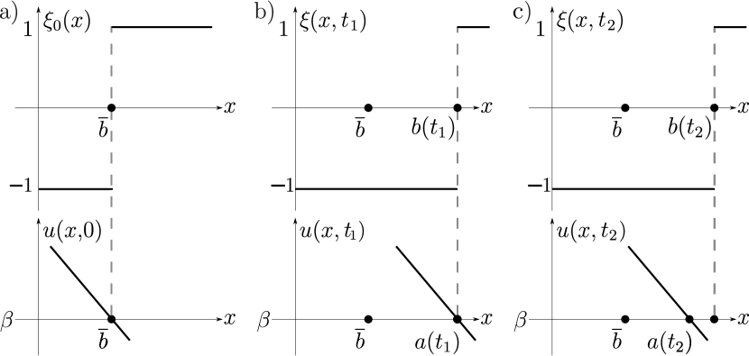
Consider a neighborhood of , and suppose at time , and are subintervals separated by a point (Figure 3a). Let for , for , and let be the unique solution of in . If at time the value of at points have already risen above , then has switched from to . These are the points such that (Figure 3b). Now if at time the value of at the switched points has fallen below again, remains switched. These are the points such that (Figure 3c). More succinctly, if and if , where .
1.6 Overview
This chapter is organized in the following way.
In Section 2 we will investigate the well-posedness of (1)–(3) for transverse initial data. For the existence of solutions and their continuous dependence on initial data was established in [11], uniqueness of the solution in [20] and the analogous results for systems of equations in [21]. Preliminary results for were obtained in [22].
In Section 3 we consider the regularity of solutions , in particular, whether the generalized derivatives and are uniformly bounded. We will summarize the results of [23], where the authors proved that these derivatives are locally bounded in a neighborhood of a point not on the free boundary. They also showed that this bound depends on the parabolic distance to the parts of the free boundary that do not contain the sets or .
2 Transverse Initial Data
2.1 Setting of a Model Problem
In this section we will discuss the well-posedness of problem (1)–(3) under the assumption that is transverse with respect to , a notion which we will make precise shortly. In order to illustrate the main ideas, we will treat the following model problem in detail and then discuss generalizations at the end of this section (see Subsection 2.4). Let be two constants, and let the hysteresis branches be given by and . Consider the prototype problem
| (6) | |||
| (7) | |||
| (8) |
We will treat in Subsection 2.2 (see [11, 20]) and (see [22]) in Subsection 2.3. Throughout this subsection we will always assume that and are consistent with each other, i.e., if (or ), then (or ). In particular, this means that for every , is continuous from the right as a function of .
Since in general , we will look for solutions in the Sobolev space with . This is the space consisting of functions with two weak spatial derivatives and one weak time derivative from (see [25, Chapter 1]). If , then for every the trace is well defined and (see, e.g., [25, p. 70]). To ensure that is regular enough to define the spatial transversality property, we henceforth fix a such that . It follows that if , then and , where is the standard Hölder space (see [26, Section 4.6.1]).
The subspace of functions with homogeneous Neumann boundary conditions is a well-defined subspace, and in this section we always assume that .
Definition 2.1
We note that if , then is a measurable function on (see [1, Section VI.1]).
2.2 Case
Let and be given by (5).
Definition 2.2
Let . We say is transverse with respect to if the following hold:
-
(1)
There is a such that and .
-
(2)
If , then .
Definition 2.3
A solution is called transverse if for all , is transverse with respect to .
Theorem 2.4 (See [11, Theorems 2.16 and 2.17])
Let be transverse with respect to . Then there is a such that the following hold:
- (1)
- (2)
- (3)
Let us define the closed, convex, bounded subset of
For any , define the function
| (9) |
Let be the solution to problem (6)–(8) with nonlinearity in place of . We claim that can be chosen small enough such that the configuration of is defined by a unique discontinuity point . Note that we do not yet claim that .
To prove the claim, first fix . It is a result of classical parabolic theory [25, Chapter 4] that for all
| (10) |
where depend only on and . The claim now follows from (10) with the help of the implicit function theorem.
Observe that is a solution of problem (6)–(8) if , i.e., . We therefore look for a fixed point of the map , .
Consider and define via similarly to (9), and let be the corresponding solutions. Observe that only if , in particular,
| (11) |
Applying (10) again, and using and the implicit function theorem, we see that the left hand side of (11) bounds . One can additionally show that bounds , hence
| (12) |
In particular (12) shows that is a continuous map on . Moreover, one can use (10) to show that is bounded in , and since is compactly embedded into , the Schauder fixed point theorem implies that has a fixed point.
Theorem 2.5 (see [20, Theorem 2.2])
We prove the theorem by expressing solutions as a convolution with the Green function for the heat equation with Neumann boundary conditions. Let us use this function to estimate the solution of the heat equation with zero initial data, Neumann boundary conditions, and the right hand side :
| (13) |
Also note that satisfies the inequality (see, e.g., [27])
| (14) |
where does not depend on , , or .
Similarly to the proof of Theorem 2.4, for every the integral of over is bounded by and hence by and hence by . Combining this with (13) and (14), and taking the supremum over we get
where does not depend on . Thus for small enough. A passage to arbitrary is standard.
Theorem 2.6 (See [11, Theorem 2.9])
The crux of the proof is showing that for sufficiently large , all the solutions exist on the same time interval . To this end we note that we have in fact given an explicit construction of , and that this depends on , , and if , also on . Hence for and close enough to and in their respective norms, the same can be used.
2.3 Case
For the case a notion of transversality has been studied in a model problem. For clarity we will define transversality for the case where the threshold is adjoined to the free boundary between and , and is not. The general case is treated similarly. In what follows, let denote the topological interior of a subset , and let be defined similarly to but taking instead of . In [22] the existence and uniqueness of solutions were studied for initial data transverse in the following sense (see Figure 4a and 4b, and recall that is given by (5)).
Definition 2.7
We say the function is transverse with respect to if the following hold:
-
(1)
and are measurable, , , and has zero Lebesgue measure.
-
(2)
for .
-
(3)
for .
-
(4)
If , then there is a neighbourhood of , a set , a , and a map such that
-
(4.a)
is a composition of a translation and a rotation and
-
(4.b)
There is a continuous function such that the configuration function in (which we denote by , ) is given by
-
(4.c)
, which we write as , satisfies .
-
(4.a)

We observe that in Subsection 2.2, the boundary between and was a single point . But when , this boundary is assumed to have the structure of a continuous codimension submanifold in a neighborhood of a point on the free boundary where takes a threshold value. Also note that for non-transversality can be caused by the geometry of in addition to the possible degeneracy of (see Figure 4c and Subsection 2.4 for further discussion).
Theorem 2.8 (see [22, Theorems 3.18 and 3.19])
The main ideas of the proof are similar to those for the case . Since is transverse in the 1d sense for every , one can prove continuity of a map that now maps functions () to solutions of problem (6)–(8) with the right hand side . Estimate (10) implies that , and the compactness of the embedding and the Schauder fixed point theorem together imply that has a fixed point in .
2.4 Generalizations and Open Problems
Let us list some generalizations for the case .
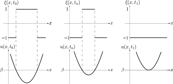
Change of topology. Suppose becomes non-transverse at some time in the sense of Definition 2.2. Then one of two possibilities arise. Either has touched a threshold with zero spatial derivative at some point in , or this is not the case but . In the latter case, one can continue the solution, and it remains unique, by redefining the problem effectively without hysteresis [11, Theorem 2.18]. We say that the topology of the hysteresis has changed at time , in the sense that transitions from piecewise constant to uniformly constant.
Continuous dependence on initial data. If is a solution such that the topology has changed for some , then need not continuously depend on the initial data since a sequence of approximating solutions may become non-transverse at moments with and (the dashed line in Figure 5). But if we also assume that each is a transverse solution, then solutions do depend continuously on their initial data.
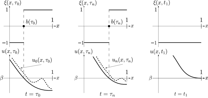
Finite number of discontinuities. The results in Subsection 2.2 remain valid if the hysteresis topology is defined by finitely many discontinuity points. The hysteresis changing topology in the sense we described for one point of discontinuity corresponds to these points merging together in the general case (see Figure 6).
General nonlinearity. The results in this section also hold for the more general problem (1)–(3). First one must assume that is locally Lipschitz and dissipative (see [11, Condition 2.11]). With such an , and if and are locally Hölder continuous, then transverse solutions exist and can be continuted up to a maximal interval of transverse existence. If one additionally assumes that transverse solutions are unique, they can be shown to continuously depend on their initial data. To prove the uniqueness of solutions the authors of [20, 22] make the stronger assumption on and , namely that
for in a left neighborhood of , with and , plus an analogous inequality for and a right neighborhood of . This condition covers the case where and are the stable branches in the slow-fast approximation as in Figure 2 (see the appendix of [20] for further discussion).
Systems of equations. In [21, Theorem 2.1], the results of Subsection 2.2 were generalized to systems of equations of the type in problem (1)–(3). It was also shown therein that problem (1)–(3) can be coupled to ordinary differential equations to cover the Hoppensteadt–Jäger model from [6, 7].
Let us conclude this subsection by discussing an open problem.
Open problem. In Figure 4c, one can see that for every , is transverse in the 1d sense (with two discontinuties), but since the free boundary cannot be represented as a graph with codomain at the point , this initial data is not transverse. Whether Definition 2.7 can be generalized to include such cases is the subject of future work, and at this stage the authors strongly suspect that item 4 of Definition 2.7 can be replaced by the following statement: if , then . In other words, the assumption that the free boundary is a graph is not necessary, and hence Figure 4c would also be transverse. This question is intimately linked to the topology of the free boundary. Whether solutions can be continued to a maximal interval of existence and how to pose continuous dependence of initial data is unclear for the quite general conditions on and in Definition 2.7. These questions also apply to the case where and has infinitely many discontinuities.
3 Regularity of Strong Solutions
To begin with let us discuss what we mean by regularity of solutions in this context. First observe that we cannot expect a classical solution since has a jump discontinuity. Therefore the “optimal” regularity we expect is . In this section we obtain “locally”, for points outside of the static part of the free boundary. We will also assume the following condition:
Condition 3.1
and .
Let us introduce the notation and observe that is smooth on the interior of .
The free boundary is defined as the set . Moreover, we define and . Note that both and have zero Lebesgue measure whenever is a solution of problem (6)–(8). This follows from the fact that a.e. on and Condition 3.1 (see Alt’s argument in the introduction and [12]).
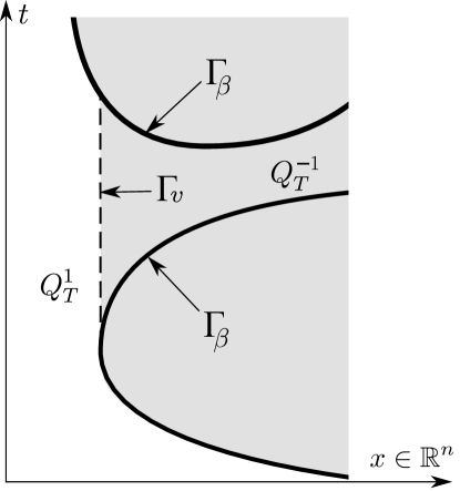
The estimates we obtain will depend critically on the static part of the free boundary . If , then and by continuity of , for sufficiently small. This means and so if we draw the -axis vertically as in Figure 7, looks like a vertical strip.
Next we recall the definition of a parabolic cylinder
We define the parabolic distance between and a set as
This is all the notation we need to state the main result of [23].
Theorem 3.2 (see [23, Theorem 2.3])
To explain the main ideas in the proof we define some further notation. Let and , with and defined similarly. Furthermore, define and .
The crucial point in the proof is the quadratic growth estimate
| (15) |
and (the estimate on is similar). The main tool for showing the quadratic bound (15) is the local rescaled version of the Caffarelli monotonicity formula, see [28, 23, 29].
Furthermore, the quadratic growth estimate (15) implies the corresponding linear bound for
| (16) |
with . The dependence of and on the distance in (15) and (16) arises due to the monotonicity formula. Near neither the local rescaled version of Caffarelli’s monotonicity formula nor its generalizations (such as the almost monotonicity formula) are applicable to the positive and negative parts of the spatial directional derivatives , with .
Besides estimates (15) and (16), one also needs information about the behaviour of near . Although may have jumps across the free boundary, one can show that is a continuous function in a neighborhood of . In addition, the monotonicity of the jumps of in the -direction provides one-sided estimates of near and . Combining these results with the observation that on , and on gives
| (17) |
Inequalities (15)–(17) allow one to apply methods from the theory of free boundary problems (see, e.g., [18, 19]) and estimate and for a.e. .
4 Non-Transverse Initial Data
4.1 Setting of a Problem
In this section we summarize the recent work [24], where the nontransverse case is analyzed for , and indicate directions for further research. We will be interested in the behavior of solutions near one of the thresholds, say . Therefore, we set and (see Figure 8)
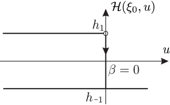
and assume that the initial data satisfy in a small neighborhood of the origin, everywhere outside of the origin, for , and for . In particular, we assume . In this situation, the theorems in Section 2.2 are not applicable. Hence, to understand the dynamics of the solution near the origin, we approximate the continuous equation (6) by its spatial discretization and the initial data by the discrete quadratic function. Namely, we choose a grid step , set , , and consider the system of infinitely many ordinary differential equations with hysteresis
| (18) |
supplemented by the nontransverse (quadratic) initial data
| (19) |
Here we do not explicitly indicate the dependence of on , assuming that if for all and otherwise. As before, we assume that .
Due to [24, Theorem 2.5], problem (18), (19) admits a unique solution in the class of functions satisfying
with some and . Thus, we are now in a position to discuss the dynamics of solutions for each fixed grid step and analyze the limit .
First, we observe that in (18), (19) can be scaled out. Indeed, setting
| (20) |
reduces problem (18), (19) to the equivalent one
| (21) |
Using the comparison principle, it is easy to see that if , then for all and and, therefore, no switchings happen for . Let us assume that
| (22) |
It is easy to show that for all and . However, some nodes can now reach the threshold and switch the hysteresis. The main question is which nodes do this and according to which law.
4.2 Numerical Observations
The following pattern formation behavior is indicated by numerics (see Figure 9).

As time goes on, the spatial profile of forms two symmetric hills propagating away from the origin. At the same time, the whole spatial profile oscillates up and down (never exceeding the threshold ) and touches the threshold in such a way that
| (23) |
where and are integers denoting the number of nodes in the set that switch and do not switch, respectively, on the time interval . In [24], such a spatio-temporal pattern was called rattling.
A more specific pattern occurs if , where and are co-prime integers. In this case, for any large enough, the set contains exactly nodes that switch and nodes that do not switch on the time interval .
If a node switches on the time interval , then we denote its switching moment by ; otherwise, set . In particular, finite values of characterize the propagation velocity of the two hills mentioned above. Numerics indicates that, for the nodes where is finite, we have
| (24) |
and
| (25) |
where do not depend on and . In particular, (24) and (25) mean that the hills propagate with velocity of order , while the cavity between the hills has a bounded steepness, which distinguishes the observed phenomenon from the “classical” traveling wave situation.
4.3 Rigorous Result
The recent work [24] provides a rigorous analysis of the rattling in the case , where, according to (24), all the nodes are supposed to switch at time moments satisfying
| (26) |
where does not depend on . In [24], the authors found the coefficient and proved that if finitely many nodes , , switch at time moments satisfying (26), then all the nodes , , switch at time moments satisfying (26) (see the rigorous statement below). One of the main tools in the analysis is the so-called discrete Green function that is a solution of the problem
| (27) |
The important property of the discrete Green function is the following asymptotics proved in [30]:
| (28) |
where
| (29) |
and does not depend on .
Now if we (inductively) assume that the nodes switched at the moments satisfying (26), while no other nodes switched on the time interval , then the dynamics of the node for (and until the next switching in the system occurs) is given by
| (30) |
At the (potential) switching moment , the relations (), equality (30), the Taylor formula, and asymptotics (28) yield
| (31) | ||||
where
and “l.o.t.” stands for lower order terms that we do not explicitly specify here. Note that is the Riemann sum for the integral
| (32) |
Therefore, equality (31) can be rewritten as
| (33) |
It is proved in [24] that there exists a unique for which the coefficient at in (33) vanishes. The most difficult part is to analyze the lower order terms in (33) that involve:
- (1)
-
(2)
the remainder in the asymptotic (28) for the discrete Green function ,
-
(3)
the remainders arising from approximating the integral by the Riemann sum .
In particular, one has to prove that if for , then the lower order terms vanish for specified above and . This allows one to continue the inductive scheme and (after an appropriate analysis of the nodes for ) complete the proof.
The rigourous formulation of the main result in [24] is as follows.
Theorem 4.1 (see [24, Theorem 3.2])
Assume that (22) holds and that . Let be a unique root of the equation
| (34) |
with given by (32). Then there exists a constant and a function both explicitly constructed with the following property. If
| (35) | ||||
then each node , , switches; moreover, the switching occurs at a time moment satisfying (26) with and as in (35).
We note that the explicit formula (30) for the solution allows one to verify the fulfillment of finitely many assumptions (35) numerically with an arbitrary accuracy for any given values of and . The graphs in Figure 10 taken from [24] represent the values of , , and that fulfill assumption (35) for and .

4.4 Open Problems
To conclude this section, we indicate several directions of further research in the nontransverse case.
Case . In this case, one has to additionally prove a specific switching pattern (23). We expect that the tools developed in [24] will work for rational . The irrational case appears to be a much more difficult problem.
Multi-dimensional case. Numerics indicates that the behavior analogous to (23) occurs in higher spatial dimensions for different kinds of approximating grids. Figure 11 illustrates the switching pattern for a two-dimensional analog of problem (21), where the Laplacian is discretized on the square and triangular lattices, respectively.

Limit . We introduce the function
(which is piecewise constant in for every fixed ). Making the transformation inverse to (20) and assuming (23) and (24), we can deduce that, as , the function approximates a smooth function , which satisfies for . In other words, sticks to the threshold line on the expanding interval .
Similarly to , we consider the function
which is supposed to approximate the hysteresis in (6). We see that the spatial profile of for is a step-like function taking values and on alternating intervals of length of order . Hence, it has no pointwise limit as , but converges in a weak sense to the function given by for and for . We emphasize that does not depend on (because does not). On the other hand, if , the hysteresis operator in (6) cannot take value by definition, which clarifies the essential difficulty with the well-posedness of the original problem (6) in the nontransverse case. To overcome the non-wellposedness, one need to allow the intermediate value for the hysteresis operator, cf. the discussion of modified hysteresis operators due to Visintin and Alt in the introduction. A rigorous analysis of the limit is an open problem, which may lead to a unique “physical” choice of an appropriate element in the multi-valued Visintin’s hysteresis in Definition 1.2.
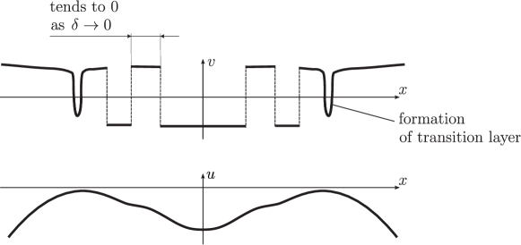
Rattling in slow-fast systems. One may think that the rattling occurs exclusively due to the discontinuous nature or hysteresis. This is not quite the case. Consider an equation of type (6) with the hysteresis replaced by the solution of a bistable ordinary differential equation of type (4), e.g.,
| (36) |
Numerical solution of system (36) with a nontransverse initial data and near the origin reveals a behavior analogous to that for a spatially discrete system (see Figure 12). As the spatial profile of touches the threshold at some point , the spatial profile of forms a peak-like transition layer around that rapidly converges to a plateau. Thus, as time goes on, the spatial profile of converges to a step-like function taking values and on alternating intervals, whose length tends to zero as . A rigorous analysis of the limit is an open problem.
Acknowledgements
The authors are grateful for the support of the DFG project SFB 910 and the DAAD project G-RISC. The work of the first author was partially supported by the Berlin Mathematical School. The work of the second author was partially supported by the DFG Heisenberg Programme. The work of the third author was partially supported by Chebyshev Laboratory (Department of Mathematics and Mechanics, St. Petersburg State University) under RF Government grant 11.G34.31.0026, JSC “Gazprom neft”, by the Saint-Petersburg State University research grant 6.38.223.2014 and RFBR 15-01-03797a.
References
- [1] A. Visintin, Differential Models of Hysteresis. Applied Mathematical Sciences, Berlin Heidelberg: Springer-Verglag, 1994.
- [2] P. Krejčí, Hysteresis, Convexity and Dissipation in Hyperbolic Equations. GAKUTO International series, Gattötoscho, 1996.
- [3] M. Brokate and J. Sprekels, Hysteresis and Phase Transitions. Applied Mathematical Sciences, New York: Springer-Verlag, 1996.
- [4] A. Visintin, “Ten issues about hysteresis,” Acta Applicandae Mathematicae, vol. 132, no. 1, pp. 635–647, 2014.
- [5] A. Visintin, “P.D.E.s with hysteresis 30 years later.,” Discrete Contin. Dyn. Syst., Ser. S, vol. 8, no. 4, pp. 793–816, 2015.
- [6] F. Hoppensteadt and W. Jäger, “Pattern Formation by Bacteria,” in Biological Growth and Spread (W. Jäger, H. Rost, and P. Tautu, eds.), vol. 38 of Lecture Notes in Biomathematics, pp. 68–81, Springer Berlin Heidelberg, 1980.
- [7] F. Hoppensteadt, W. Jäger, and C. Pöppe, “A hysteresis model for bacterial growth patterns,” in Modelling of Patterns in Space and Time (W. Jäger and J. D. Murray, eds.), vol. 55 of Lecture Notes in Biomathematics, pp. 123–134, Springer Berlin Heidelberg, 1984.
- [8] A. Marciniak-Czochra, “Receptor-based models with hysteresis for pattern formation in hydra,” Mathematical Biosciences, vol. 199, no. 1, pp. 97 – 119, 2006.
- [9] A. Köthe, Hysteresis-Driven Pattern Formation in Reaction-Diffusion-ODE Models. PhD thesis, University of Heidelberg, 2013.
- [10] M. Krasnosel’skii, M. Niezgodka, and A. Pokrovskii, Systems with Hysteresis. Springer Berlin Heidelberg, 2012.
- [11] P. Gurevich, S. Tikhomirov, and R. Shamin, “Reaction diffusion equations with spatially distributed hysteresis,” Siam J. of Math. Anal., vol. 45, no. 3, pp. 1328–1355, 2013.
- [12] H. W. Alt, “On the thermostat problem,” Control Cybern., vol. 14, no. 1-3, pp. 171–193, 1985.
- [13] A. Visintin, “Evolution problems with hysteresis in the source term,” SIAM J. Math. Anal., vol. 17, no. 5, 1986.
- [14] T. Aiki and J. Kopfová, “A mathematical model for bacterial growth described by a hysteresis operator,” in Recent Advances in Nonlinear Analysis, pp. 1–10, 2008.
- [15] P. Krejčí, “The hysteresis limit in relaxtion oscillation problems,” J. Physics.: Conf. Ser., no. 22, pp. 103–123, 2005.
- [16] E. Mischenko and N. Rozov, Differential Equations with Small Parameters and Relaxation Oscillations. New York: Plenum, 1980.
- [17] C. Kuehn, Multiple Time Scale Dynamics, vol. 191 of Applied Mathematical Sciences. Springer International Publishing, 2015.
- [18] D. Apushkinskaya and N. Uraltseva, “Uniform estimates near the initial state for solutions of the two-phase parabolic problem.,” St. Petersbg. Math. J., vol. 25, no. 2, pp. 195–203, 2014.
- [19] H. Shahgholian, N. Uraltseva, and G. S. Weiss, “A parabolic two-phase obstacle-like equation,” Adv. Math., vol. 221, no. 3, pp. 861–881, 2009.
- [20] P. Gurevich and S. Tikhomirov, “Uniqueness of transverse solutions for reaction-diffusion equations with spatially distributed hysteresis,” Nonlinear Anal., vol. 75, pp. 6610–6619, December 2012.
- [21] P. Gurevich and S. Tikhomirov, “Systems of reaction-diffusion equations with spatially distributed hysteresis.,” Mathematica Bohemica (Proc. Equadiff 2013), vol. 139, no. 2, pp. 239–257, 2014.
- [22] M. Curran, “Local well-poseness of a reaction-diffusion equation with hysteresis.,” Master’s thesis, Fachbereich Mathematik und Informatik, Freie Universität Berlin, 2014.
- [23] D. Apushkinskaya and N. Uraltseva, “On regularity properties of solutions to the hysteresis-type problem,” Interfaces and Free Boundaries, vol. 17, no. 1, pp. 93–115, 2015.
- [24] P. Gurevich and S. Tikhomirov, “Spatially discrete reaction-diffusion equations with discontinuous hysteresis,” ArXiv:1504.02385 [math.AP], 2015.
- [25] O. Ladyzhenskaya, V. Solonnikov, and N. Uraltseva, Linear and Quasilinear Equations of Parabolic Type. Providence, Rohde Island: American Mathematical Society, 1968.
- [26] H. Triebel, Interpolation Theory, Function Spaces, Differential Operators. Carnegie-Rochester Conference Series on Public Policy, North-Holland Publishing Company, 1978.
- [27] S. Ivasishen, “Green’s matrices of boundary value problems for Petrovskii parabolic systems of general form. ii,” Math. USSR-Sb, no. 4, pp. 461–498, 1981.
- [28] L. Caffarelli and S. Salsa, A Geometric Approach to Free Boundary Problems. Graduate studies in mathematics, American Mathematical Soc., 2005.
- [29] D. Apushkinskaya, H. Shahgholian, and N. Uraltseva, “Boundary estimates for solutions of the parabolic free boundary problem,” Journal of Mathematical Sciences, vol. 115, no. 6, pp. 2720–2730, 2003.
- [30] P. Gurevich, “Asymptotics of parabolic Green’s functions on lattices,” ArXiv:1504.02673 [math.AP], 2015.