A family of lowered isothermal models

Abstract

We present a family of self-consistent, spherical, lowered isothermal models, consisting of one or more mass components, with parameterized prescriptions for the energy truncation and for the amount of radially biased pressure anisotropy. The models are particularly suited to describe the phase-space density of stars in tidally limited, mass-segregated star clusters in all stages of their life-cycle. The models extend a family of isotropic, single-mass models by Gomez-Leyton and Velazquez, of which the well-known Woolley, King and Wilson (in the non-rotating and isotropic limit) models are members. We derive analytic expressions for the density and velocity dispersion components in terms of potential and radius, and introduce a fast model solver in python (limepy), that can be used for data fitting or for generating discrete samples.

1 Introduction

The evolution of globular clusters (GCs) is the result of an interplay between stellar astrophysics (stellar and binary evolution, stellar mergers, etc.), dynamical two-body relaxation and the interaction with the tidal field of their host galaxy (Heggie & Hut, 2003). Despite this plethora of physical processes at work on their respective time-scales, the instantaneous surface brightness profiles and kinematics of GCs are well described by relatively simple distribution function (DF) based models that need very few assumptions (Gunn & Griffin, 1979; Meylan & Heggie, 1997; Zocchi, Bertin & Varri, 2012).

The relative simplicity of GC properties is owing to the absence of gas and non-baryonic dark matter and the collisional nature of their evolution, which drives them to tractable properties, such as spherical symmetry, isotropy and (quasi-)equipartition between different mass species (e.g. Spitzer, 1987). Because the relaxation time-scale of GCs is much longer than their dynamical time, their instantaneous properties can be described by models that satisfy the collisionless Boltzmann equation (see e.g. Chapter 8 in Bertin, 2014).

Two-body interactions in GCs evolve the velocity distribution of stars towards a Maxwell-Boltzmann distribution, at least in the core, where the relaxation time-scale is short. Models with isothermal cores are therefore a good choice for fitting properties of GCs. An obvious starting point for a discussion on model choice is, therefore, the isothermal model. This model has an infinite spatial extent and infinite mass (Chandrasekhar, 1939) and to make the model applicable to real star clusters, the assumption of the idealized Maxwell-Boltzmann distribution of velocities needs to be relaxed. This can be done by changing the model such that stars have a finite escape velocity. Woolley (1954) developed such a model by simply ‘lowering’ the (specific) energy $E$ by a constant. The DF, which describes the density in six-dimensional phase-space as a function of $E$, is then simply $f(E)=A\exp[-(E-\phi(r_{\rm t}))/s^{2}]$, for $E\leq\phi(r_{\rm t})$, and $f(E)=0$ for $E>\phi(r_{\rm t})$. Here $s$ is a velocity scale, which in the isothermal model equals the one-dimensional velocity dispersion and $E$ is reduced by the specific potential at the truncation radius $r_{\rm t}$, $\phi(r_{\rm t})$. This truncation in energy mimics the role of tides due to the host galaxy, which makes it easier for stars to escape by reducing the escape velocity. The resulting models are nearly isothermal in the core, and have a finite mass and extent.

The DF of these models is discontinuous at $E=\phi(r_{\rm t})$. Michie (1963) and King (1966) avoided this by subtracting a constant from the DF introduced by Woolley, which makes the models continuous at $E=\phi(r_{\rm t})$. Compared to the Woolley models, the density of stars near the escape energy is reduced in these models (hereafter referred to as King models), and they display a more gentle truncation of their density profile. The resulting, more extended, low-density envelopes make these models resemble real GCs more (for an in depth discussion on the effect of the truncation on the density profiles see Hunter, 1977). The spherical, non-rotating limit of the models introduced by Wilson (1975), hereafter called Wilson models, are models that are continuous both in the DF and its derivative. This is achieved by subtracting an additional term linear in $E$ from the DF. These models are yet more spatially extended than King models. For some GCs in Local Group galaxies, the Wilson models provide a better description of the observed surface brightness profiles compared to the King models (McLaughlin & van der Marel 2005; Carballo-Bello et al. 2012 also show that models that are more extended than King models better describe the surface brightness profiles of some GCs).

An additional outcome of the two-body relaxation process is that it drives the velocity distribution of the stars towards isotropy. Isotropic models, defined by a DF that only depends on $E$, are therefore a natural choice for clusters that are in late stages of their evolution, near dissolution. At early phases, however, the velocity distribution in the outer parts is expected to be radially anisotropic. This is, first, because the (incomplete) violent relaxation process that takes place during their formation results in a halo of radial orbits (Lynden-Bell, 1967). Secondly, two-body ejections from the dense core populate the halo with radial orbits on a two-body relaxation time-scale (Spitzer & Shapiro, 1972). Michie (1963) proposed a separable DF, dependent on $E$ and on the (specific) angular momentum $J$ to introduce radial anisotropy (hereafter referred to as Michie-King models). The DF of the Michie-King models is the product of the isotropic DF with an exponential term with a $J^{2}$ dependent argument. This is similar to Eddington’s method of including radial anisotropy in the isothermal model (Eddington, 1915). As a result, the inner parts of the models remain approximately isothermal and isotropic, which is appropriate to GCs because there the relaxation time is short, and anisotropy becomes important at larger distances from the centre. Near the truncation radius the models become isotropic again as a result of the energy truncation. The latter property has a somewhat coincidental resemblance to GCs, because near the Jacobi radius the orbits of stars gain angular momentum due to the interaction with the (tri-axial) tidal potential (Oh & Lin, 1992), therewith suppressing the amount of radial anisotropy near the truncation energy. A review of the effect of anisotropy on model properties can be found in Binney (1982).

In real GCs, which contain multiple mass components, the relaxation process drives the systems towards equipartition, resulting in the heavier components being more centrally concentrated, a state which is often referred to as mass segregated. King models with different mass species were first introduced by Da Costa & Freeman (1976) and have since been applied to take into account the effects of mass segregation in mass-modelling efforts of Galactic GCs (e.g. M3: Gunn & Griffin 1979, Omega Cen: Meylan 1987 and larger samples of GCs: Pryor & Meylan 1993; Sollima et al. 2012). Mass segregation is important for almost all of the Galactic GCs, given their short relaxation time-scales, relative to their ages (Hénon, 1961; Gieles, Heggie & Zhao, 2011). Approximating multimass systems by single-mass models can lead to severe biases in the inferred properties of GCs (Shanahan & Gieles, 2015; Sollima et al., 2015) and it is, therefore, desirable to have the ability to include multiple mass components in a dynamical model of a GC.

It is our aim to develop a family of models that capture the general behaviour of collisional systems discussed above, and whose properties can be varied by parameters that can be constrained by observational data. Davoust (1977) showed that the expressions for the DF of the isotropic Woolley, King and Wilson models can be generalized by a DF in which the exponential function of $E$ is reduced by the leading orders of its series expansion. This approach was further generalized by Gomez-Leyton & Velazquez (2014, hereafter GV14), who showed that solutions in between these models can be obtained (these models are briefly reviewed in Section 2.1.3). In this paper we extend the models of GV14 to allow for the presence of (radially biased) pressure anisotropy and multiple mass components. We present an efficient Poisson solver in python to facilitate the use of these models in fitting observational data, and in drawing samples from the models, which can be used as initial conditions for numerical simulations.

The paper is organized as follows: in Section 2, we define the models and in Section 3, we illustrate their main properties. In Section 4, we present the code limepy and our conclusions and a discussion are presented in Section 5. Supporting material can be found in the appendices.

2 Model definition and scaling

2.1 Single-mass models

2.1.1 Distribution function (DF)

The DF of the single-mass family of models is

$$f(E,J^{2})=\displaystyle A\exp\left(-\frac{J^{2}}{2r_{\rm a}^{2}s^{2}}\right)E_{\gamma}\left(g,-\frac{E-\phi(r_{\rm t})}{s^{2}}\right)$$ (1)

for $E\leq\phi(r_{\rm t})$, and 0 for $E>\phi(r_{\rm t})$. The DF depends on two integrals of motion: the specific energy $E=v^{2}/2+\phi(r)$, with $v$ the velocity and $\phi(r)$ the specific potential at distance $r$ from the centre, and the norm of the specific angular momentum vector $J=|\textbf{\emph{r}}\times\textbf{\emph{v}}|=rv\sin\vartheta$, where r and v are the position vector and velocity vector, respectively, and $\vartheta$ is the angle between them. The energy $E$ is lowered by the potential at the truncation radius $\phi(r_{\rm t})$.

In equation (1) we introduced the function

$$E_{\gamma}(a,x)=\begin{cases}\exp(x)&a=0\\ \displaystyle\exp(x)P(a,x)&a>0,\end{cases}$$ (2)

where $P(a,x)\equiv\gamma(a,x)/\Gamma(a)$ is the regularized lower incomplete gamma function (see Appendix D.1 for the definition of this function and its properties). Combining the exponential and the incomplete gamma function into a single function $E_{\gamma}(a,x)$ has advantages in deriving the model properties (see GV14 and Appendix D.2 for details on the behaviour of this function).

A model is specified by three parameters: the central potential, which is a required boundary condition for solving Poisson’s equation and defines how concentrated the model is; the anisotropy radius $r_{\rm a}$, which determines the amount of anisotropy present in the system (for increasing $r_{\rm a}$ the models are more isotropic); the truncation parameter $g$, which controls the sharpness of the truncation of the model (this parameter is called $\gamma$ in GV14). The physical units of a model are defined by two scales: the velocity scale $s$, and the normalization constant $A$, which sets the phase-space density and therewith the total mass $M$. For more information regarding scales and parameters of the models we refer the reader to Section 2.1.2.

The isotropic models ($r_{\rm a}\rightarrow\infty$) and their properties are discussed in detail in GV14. For these models, and integer values of $g$, three well-known families of models are recovered: when $g=0$ we retrieve the Woolley (1954) models, for $g=1$ we recover the King models (Michie, 1963; King, 1966), and for $g=2$ we find the (isotropic, non-rotating) Wilson models (Wilson, 1975). In practice, the models defined by equation (1) are radially anisotropic for $r_{\rm a}\lesssim r_{\rm t}$, because of the $J^{2}$ dependence in the first exponential. When $g=1$, the DF is the Michie-King model (Michie, 1963), which is often used to fit GC data (e.g. Meylan, 1987; Sollima et al., 2012).

The potential $\phi(r)$ is found by solving Poisson’s equation. For the self-consistent problem we consider here, the potential is completely determined by the density $\rho$ associated with the DF. This problem is non-linear, because the DF depends on the potential. Since the models defined by equation (1) are spherically symmetric, Poisson’s equation is

$$\frac{1}{r^{2}}\frac{{\rm d}}{{\rm d}r}\left(r^{2}\frac{{\rm d}\phi}{{\rm d}r}\right) =4\pi G\rho,$$ (3)

where the density is obtained by means of an integration of the DF over all velocities

$$\rho=\int{\rm d}^{3}v\,f(E,J^{2}).$$ (4)

In Sections 2.1.3 and 2.1.4, we derive analytic expressions for $\rho$ as a function of $\phi$ and $r$. Note that only in the anisotropic case the dependence on the radial coordinate $r$ is both implicit (through $\phi$, as in the isotropic case), and explicit, i.e. $\rho(\phi,r)$. Having analytic expressions for $\rho(\phi,r)$, avoids the need of solving a double integral at each radial step, making it significantly faster to obtain the solution to Poisson’s equation. In the next section we introduce a convenient set of units to solve the model.

2.1.2 Scaling and units

To solve Poisson’s equation, we use a dimensionless (positive) energy $\hat{E}=\hat{\phi}-\hat{k}$, with dimensionless potential $\hat{\phi}=(\phi(r_{\rm t})-\phi)/s^{2}$, and $\hat{k}\equiv v^{2}/(2s^{2})$. As in King (1966), we consider the dimensionless density by normalizing $\rho$ to its central value, i.e. $\hat{\rho}=\rho/\rho_{0}$. In this way, Poisson’s equation in dimensionless form reads

$$\frac{1}{\hat{r}^{2}}\frac{{\rm d}}{{\rm d}\hat{r}}\left(\hat{r}^{2}\frac{{\rm d}\hat{\phi}}{{\rm d}\hat{r}}\right)=-9\hat{\rho}.$$ (5)

The dimensionless radius is now defined by the other scales: $\hat{r}=r/r_{\rm s}$, with $r_{\rm s}^{2}=9s^{2}/(4\pi G\rho_{0})$. This radial scale was introduced in King (1966) and is often referred to as the King radius. The factor of 9 was introduced to give $r_{\rm s}$ the meaning of a core radius, because for models with moderately high central concentration, the projected density at $r_{\rm s}$ is about one half of its central value.

The Poisson equation is solved by assuming the boundary conditions at $\hat{r}=0$: $\hat{\phi}=\hat{\phi}_{0}$ and ${\rm d}\hat{\phi}/{\rm d}r=0$. As mentioned in Section 2.1.1, the central potential $\hat{\phi}_{0}$ is one of the parameters that define the model.

2.1.3 Isotropic models

We first briefly review the isotropic version of these models, as introduced by GV14. Many quantities can be derived from the DF. The density $\rho$ is found by integrating the DF over all velocities (equation 4) and the pressure is found by taking the second velocity moment of the DF

$$\rho =(2\pi s^{2})^{3/2}A\mathcal{I}^{\rho},$$ (6)

$$\rho\sigma^{2} =(2\pi s^{2})^{3/2}s^{2}A\mathcal{I}^{\rho\sigma^{2}}.$$ (7)

Here $\sigma^{2}=3\sigma_{\rm 1d}^{2}$ is the mean-square velocity, $\sigma_{\rm 1d}$ is the one-dimensional velocity dispersion and we introduce a dimensionless density integral ($\mathcal{I}^{\rho}$) and a dimensionless pressure integral ($\mathcal{I}^{\rho\sigma^{2}}$)

$$\mathcal{I}^{\rho} =\frac{2}{\sqrt{\pi}}\int_{0}^{\hat{\phi}}{\rm d}\hat{k}\,\hat{k}^{1/2}E_{\gamma}(g,\hat{\phi}-\hat{k})=E_{\gamma}(g+\textstyle{\frac{3}{2}}\displaystyle,\hat{\phi}),$$ (8)

$$\mathcal{I}^{\rho\sigma^{2}} =\frac{4}{\sqrt{\pi}}\int_{0}^{\hat{\phi}}{\rm d}\hat{k}\,\hat{k}^{3/2}E_{\gamma}(g,\hat{\phi}-\hat{k})=3E_{\gamma}(g+\textstyle{\frac{5}{2}}\displaystyle,\hat{\phi}).$$ (9)

The results of these integrations follow straightforwardly from the convolution formula of the $E_{\gamma}(a,x)$ function (equation 105). An alternative derivation by means of fractional calculus is presented in Appendix B. The dimensionless density that appears in Poisson’s equation is therefore $\hat{\rho}=\mathcal{I}^{\rho}/\mathcal{I}_{0}^{\rho}$, where $\mathcal{I}_{0}^{\rho}$ is the result of equation (8) evaluated at $\hat{\phi}=\hat{\phi}_{0}$. The dimensionless mean-square velocity is found from $\hat{\sigma}^{2}=\sigma^{2}/s^{2}=\mathcal{I}^{\rho\sigma^{2}}/\mathcal{I}^{\rho}$.

2.1.4 Anisotropic models

Here we present the relevant quantities for the anisotropic case. The details of the derivations can be found in Appendix A, and the derivations by means of fractional calculus can be found in Appendix B. To solve the anisotropic models, we introduce $t=\cos\theta$, such that we can write the integral over the angles as $4\pi\int_{0}^{1}{\rm d}t$. We further introduce $\hat{p}=\hat{r}/\hat{r}_{\rm a}$ such that the density integral becomes

$$\mathcal{I}^{\rho} =\frac{2}{\sqrt{\pi}}\!\int_{0}^{\hat{\phi}}\!{\rm d}\hat{k}\int_{0}^{1}\!{\rm d}t\,\exp\left[\hat{k}\hat{p}^{2}(t^{2}-1)\right]\hat{k}^{1/2}E_{\gamma}(g,\hat{\phi}-\hat{k})$$

$$=\frac{2}{\sqrt{\pi}}\int_{0}^{\hat{\phi}}{\rm d}\hat{k}\,\frac{F(\hat{p}\hat{k}^{1/2})}{\hat{p}}E_{\gamma}(g,\hat{\phi}-\hat{k}).$$ (10)

Here $F(x)$ is Dawson’s integral and we refer to Appendix D.3 for some properties of this function. To first order, $F(x)\propto x$, and we thus find that for large $\hat{r}_{\rm a}$, i.e. small $\hat{p}$, equation (10) converges to the integral of the isotropic model (equation 8). The solution of the integration gives $\mathcal{I}^{\rho}$ as a function of $\hat{\phi}$ and $\hat{p}$

$$\mathcal{I}^{\rho}\!=\!\frac{E_{\gamma}(g+\textstyle{\frac{3}{2}}\displaystyle,\hat{\phi})}{1+\hat{p}^{2}}+\frac{\hat{p}^{2}}{1+\hat{p}^{2}}\frac{\hat{\phi}^{g+\tfrac{3}{2}}{{}_{1}}F_{1}(1,g+\textstyle{\frac{5}{2}}\displaystyle,-\hat{\phi}\hat{p}^{2})}{\Gamma(g+\tfrac{5}{2})}.$$ (11)

Here ${{}_{1}}F_{1}(a,b,x)$ is the confluent hypergeometric function whose properties are given in Appendix D.4. For small $\hat{p}$, the second term on the right-hand-side goes to zero and the solution converges to the isotropic result of equation (8). This expression for the density integral allows for fast computations of the right-hand-side of Poisson’s equation and facilitates efficient solving of the anisotropic models.

For the anisotropic models, we need to calculate both the radial and the tangential components of the pressure tensor, as well as the total pressure. The radial and tangential component of the velocity vector are defined as $v_{\rm r}=v\cos\theta$ and $v_{\rm t}=v\sin\theta$ and for the corresponding integrals we find

$$\displaystyle\mathcal{I}^{\rho\sigma_{\rm r}^{2}} =\frac{4}{\sqrt{\pi}}\!\int_{0}^{\hat{\phi}}\!\!\!{\rm d}\hat{k}\!\int_{0}^{1}\!\!\!{\rm d}t\,\exp\!\left[\hat{p}^{2}\hat{k}(t^{2}\!\!-\!1)\right]t^{2}\hat{k}^{3/2}E_{\gamma}(g,\hat{\phi}-\hat{k}),$$ (12)

$$\displaystyle\mathcal{I}^{\rho\sigma_{\rm t}^{2}} =\frac{4}{\sqrt{\pi}}\!\int_{0}^{\hat{\phi}}\!\!\!{\rm d}\hat{k}\!\int_{0}^{1}\!\!\!{\rm d}t\,\exp\!\left[\hat{p}^{2}\hat{k}(t^{2}\!-\!1)\right](1\!-t^{2})\hat{k}^{3/2}E_{\gamma}(g,\hat{\phi}-\hat{k}),$$ (13)

$$\displaystyle\mathcal{I}^{\rho\sigma^{2}} =\frac{4}{\sqrt{\pi}}\!\int_{0}^{\hat{\phi}}\!\!\!{\rm d}\hat{k}\!\int_{0}^{1}\!\!\!{\rm d}t\,\exp\!\left[\hat{p}^{2}\hat{k}(t^{2}\!-\!1)\right]\hat{k}^{3/2}E_{\gamma}(g,\hat{\phi}-\hat{k}).$$ (14)

By carrying out these integrals as described in Appendices A.2 and B.2, we obtain

$$\mathcal{I}^{\rho\sigma_{\rm r}^{2}} \!=\!\frac{E_{\gamma}(g+\textstyle{\frac{5}{2}}\displaystyle,\hat{\phi})}{1+\hat{p}^{2}}\!+\!\frac{\hat{p}^{2}}{1+\hat{p}^{2}}\frac{\hat{\phi}^{g+\tfrac{5}{2}}{{}_{1}}F_{1}(1,g\!+\!\tfrac{7}{2},\!-\hat{\phi}\hat{p}^{2})}{\Gamma(g+\tfrac{7}{2})},$$ (15)

$$\mathcal{I}^{\rho\sigma_{\rm t}^{2}} =\frac{E_{\gamma}(g+\textstyle{\frac{5}{2}}\displaystyle,\hat{\phi})}{1+\hat{p}^{2}}\frac{2}{(1+\hat{p}^{2})}+\frac{2\hat{p}^{2}}{1+\hat{p}^{2}}\frac{\hat{\phi}^{g+\tfrac{5}{2}}}{\Gamma(g+\tfrac{7}{2})}$$

$$\times\left[\frac{{{}_{1}}F_{1}(1,g+\tfrac{7}{2},-\hat{\phi}\hat{p}^{2})}{1+\hat{p}^{2}}+{{}_{1}}F_{1}(2,g+\tfrac{7}{2},-\hat{\phi}\hat{p}^{2})\right],$$ (16)

$$\mathcal{I}^{\rho\sigma^{2}} \!=\!\frac{E_{\gamma}(g+\textstyle{\frac{5}{2}}\displaystyle,\hat{\phi})}{1+\hat{p}^{2}}\frac{(3+\hat{p}^{2})}{(1+\hat{p}^{2})}+\frac{\hat{p}^{2}}{1+\hat{p}^{2}}\frac{\hat{\phi}^{g+\tfrac{5}{2}}}{\Gamma(g+\tfrac{7}{2})}$$

$$\times \left[\!\frac{3+\hat{p}^{2}}{1+\hat{p}^{2}}{{}_{1}}F_{1}(1,g\!+\!\tfrac{7}{2},\!-\hat{\phi}\hat{p}^{2})\!+\!2{{}_{1}}F_{1}(2,g\!+\!\tfrac{7}{2},\!-\hat{\phi}\hat{p}^{2})\right]\!.$$ (17)

Note that the expression for $\mathcal{I}^{\rho\sigma_{\rm r}^{2}}$ resembles the expression for $\mathcal{I}^{\rho}$ of equation (11), in the sense that the functional form is the same, but all arguments and the power index that include $g$ are increased by 1. We already saw a similar resemblance between $\mathcal{I}^{\rho}$ and $\mathcal{I}^{\rho\sigma^{2}}$ in the isotropic case (equations 8 and 9, respectively).

With these expressions for the density and pressure integrals, we defined most of the properties of these models that are of direct relevance for comparison to data. In Section 4.2, we discuss how the projected quantities can be derived.

2.1.5 Limits

In this section we consider some limits of the models. In the core, where $\hat{p}$ is small ($\hat{r}\ll\hat{r}_{\rm a}$), the model is isotropic. This is because the second terms in equations (11), (15), (16) and (17) vanish due to the multiplication by $\hat{p}^{2}$.

Near the truncation radius the models behave like polytropes and are, therefore, also isotropic, because

$$\lim_{\hat{\phi}\rightarrow 0}{{}_{1}}F_{1}(1,a\!+\!1,-\hat{p}^{2}\hat{\phi}) =1,$$ (18)

$$\lim_{\hat{\phi}\rightarrow 0}E_{\gamma}(a,\hat{\phi}) =\frac{\hat{\phi}^{a}}{\Gamma(a+1)},$$ (19)

and the $\hat{p}$ dependence disappears. In this regime, we find

$$\lim_{\hat{\phi}\rightarrow 0}\hat{\rho} =\frac{\hat{\phi}^{g+3/2}}{\Gamma(g+5/2)},$$ (20)

$$\lim_{\hat{\phi}\rightarrow 0}\hat{\rho}\hat{\sigma}^{2} =3\frac{\hat{\phi}^{g+5/2}}{\Gamma(g+7/2)},$$ (21)

$$\lim_{\hat{\phi}\rightarrow 0}\hat{\rho}\hat{\sigma}_{\rm r}^{2} =\frac{1}{3}\lim_{\hat{\phi}\rightarrow 0}\hat{\rho}\hat{\sigma}^{2}=\frac{1}{2}\lim_{\hat{\phi}\rightarrow 0}\hat{\rho}\hat{\sigma}_{\rm t}^{2}.$$ (22)

This suppression of the velocity anisotropy near the truncation radius results naturally from the mathematical definition of the truncation, and is appropriate for tidally truncated systems (Oh & Lin, 1992). In $N$-body models a tangentially biased anisotropy is observed near $r_{\rm t}$ (Sollima et al., 2015), which cannot be reproduced by the models presented here. However, it is likely that most of the stars with tangentially biased velocities are above the escape energy, so-called potential escapers and these are not considered by these models, nor any other model we are aware off.

Models with $\hat{\phi}_{0}\rightarrow 0$ are close to pure polytropes over their entire radial range. In this regime, and for $g=7/2$ (i.e. a polytropic index $n=5$, equation 20), we recover the Plummer (1911) model, which is infinite in extent ($\rho\propto r^{-5}$ at large radii), but finite in mass. Polytropes with $n\geq 5$ (i.e. $g\geq 7/2$) are infinite in extent and will not be considered here. For $g<7/2$ models can have a finite $r_{\rm t}$ depending on both $\hat{\phi}_{0}$ and $r_{\rm a}$ (see GV14 and Section 3).

In the cores of models with $\hat{\phi}_{0}\gg 0$ the DF approaches the isothermal sphere, because

$$\lim_{\hat{\phi}\rightarrow\infty}E_{\gamma}(a,\hat{\phi}) =\exp(\hat{\phi}).$$ (23)

Models with $g\rightarrow\infty$ also approach the isothermal sphere. To conclude, these models approach the isothermal sphere in the limit of $\hat{\phi}_{0}\rightarrow\infty$, independent of $g$, but also in the limit of $g\rightarrow\infty$, independent of $\hat{\phi}_{0}$.

2.2 Multimass models

It is possible to consider models with multiple mass components, by considering the DF as the sum of DFs of the form of equation (1), each of which describes a different mass component with a mass-dependent velocity scale parameter. The first to do this were Da Costa & Freeman (1976), who calculated multimass King models. For a multimass model with $N_{\rm comp}$ mass components, $2N_{\rm comp}+2$ parameters are required in addition to the ones introduced in Section 2.1.1 for single-mass models. These additional parameters are the values for the component masses $m_{j}$, the amount of mass in each component $M_{j}$, $\delta$ and $\eta$. The latter two parameters set the mass dependence of the velocity scale $s_{j}$ and the anisotropy radius of each component $\hat{r}_{{\rm a},j}$, for which we adopt power-law relations

$$s_{j} =s\mu_{j}^{-\delta},$$ (24)

$$\hat{r}_{{\rm a},j} =\hat{r}_{\rm a}\mu_{j}^{\eta}.$$ (25)

Here $\mu_{j}=m_{j}/\bar{m}$ is the dimensionless mass of component $j$ and $\bar{m}$ is the central density weighted mean-mass

$$\bar{m}=\frac{\sum_{j}m_{j}\rho_{0j}}{\sum_{j}\rho_{0j}}.$$ (26)

Note that in the multimass models, the values of $s$ and $\hat{r}_{\rm a}$ are the velocity scale and anisotropy radius corresponding to $\bar{m}$. The definitions of $\delta$ and $\eta$ are such that the anisotropy profiles are approximately mass independent when $\delta=\eta$ (see equation 1). The typical values considered for these parameters are $\delta=1/2$ and $\eta=0$.

We notice that in the limit of infinite $\hat{\phi}_{0}$ the velocity scale $s_{j}$ approaches the one-dimensional velocity dispersion of mass component $j$, $\sigma_{{\rm 1d},j}$, hence the traditional assumption for $\delta=1/2$ implies equipartition ($m_{j}s_{j}^{2}=\bar{m}\sigma_{{\rm 1d},j}^{2}=$ constant). However, it is important to keep in mind that for multimass models with typical and realistic values of $\hat{\phi}_{0}$, the velocity dispersion of each component in the centre is smaller than $s_{j}$ and, therefore, there is no equipartition (see Section 3.2.1 and Merritt 1981; Miocchi 2006).

To solve a multimass model self-consistently, we compute the density for each mass component as in equation (4) and add all components on the right-hand-side of Poisson’s equation. The detailed procedure is described in Gunn & Griffin (1979), and here we only briefly summarize the required steps. The dimensionless Poisson equation to solve is

$$\hat{\nabla}^{2}\hat{\phi}=-9\sum_{j}\alpha_{j}\hat{\rho}_{j},$$ (27)

where $\alpha_{j}$ is the ratio of the central density of the $j$-th mass component to the total central density, such that

$$\sum_{j}\alpha_{j}=\sum_{j}\frac{\rho_{0j}}{\rho_{0}}=1$$ (28)

and

$$\hat{\rho}_{j}=\frac{\rho_{j}}{\rho_{0j}}=\frac{\mathcal{I}^{\rho}(\mu^{2\delta}\hat{\phi},\hat{r})}{{\mathcal{I}^{\rho}(\mu^{2\delta}\hat{\phi}_{0},0)}}.$$ (29)

By considering multiple mass components, we introduce an eigenvalue problem in the solution of Poisson’s equation, because the values of $\rho_{0j}$ that yield the desired ${M}_{j}$ values are not known a priori. Therefore, as a first step to solve the model, we assume that $\alpha_{j}={M}_{j}/\sum_{j}M_{j}$, and we obtain the solution by iteration (see Section 4 for details).

2.3 Normalization and potential energy

In solving the models we have chosen to define the dimensionless quantities in terms of the density scale $\rho_{0}$ and the velocity scale $s$ (Section 2.1.2). In some cases it is useful to have an expression for the normalization constant $A$ in the DF (equation 1), for example, when fitting models to discrete data. From equation (6) we find that $A$ relates to the other scales as

$$A =\frac{\rho_{0}}{(2\pi s^{2})^{3/2}\mathcal{I}_{0}^{\rho}}.$$ (30)

For the multimass models there is a normalisation for each component, $A_{j}$. The relation with the mass scale $M_{\rm s}=M/\hat{M}$ is $M_{\rm s}=r_{\rm s}^{3}\rho_{0}=r_{\rm s}^{3}(2\pi s^{2})^{3/2}A\mathcal{I}_{0}^{\rho}$, where we introduced $\hat{M}=\int\hat{\rho}{\rm d}^{3}\hat{r}$.

The total dimensionless (positive) gravitational energy $\hat{U}$ of the model is calculated from integrating the potential (King, 1966)

$$\hat{U} =\frac{1}{2}\int_{0}^{\hat{M}}{\rm d}\hat{m}\,\hat{\phi}+\frac{\hat{G}\hat{M}^{2}}{2\hat{r}_{\rm t}}.$$ (31)

The second term has to be added because $\hat{\phi}$ is a lowered potential. Note that this integration of $\hat{\phi}$ over mass is readily obtained from solving Poisson’s equation.

3 Model properties

3.1 Single-mass models

3.1.1 Density and velocity dispersion profiles

In Fig. 1, we show the density profiles, the velocity dispersion profiles, and the anisotropy profiles for isotropic and anisotropic models with different values of the truncation parameter $g$. The anisotropy profile is computed from $\sigma_{\rm t}^{2}$ and $\sigma_{\rm r}^{2}$ as

$$\beta=1-\frac{\sigma_{\rm t}^{2}}{2\sigma_{\rm r}^{2}}.$$ (32)

In the case of isotropy $\beta=0$, $0<\beta\leq 1$ indicates radially biased anisotropy (with $\beta=1$ implying fully radial orbits) and for tangentially biased anisotropy $\beta<0$. Because $\beta$ is a measure of anisotropy locally, we also quantify the total amount of anisotropy with

$$\kappa=\frac{2K_{\rm r}}{K_{\rm t}},$$ (33)

introduced by Polyachenko & Shukhman (1981). Here $K_{\rm r}$ and $K_{\rm t}$ are the radial and tangential components of the kinetic energy, respectively. For isotropic models $\kappa=1$, and for radially biased anisotropic models $\kappa>1$. Polyachenko & Shukhman (1981) found that for $\kappa>1.7\pm 0.25$ radial orbit instability occurs. We use this criterion to check the stability of the anisotropic models we calculate.

Figure 1: Dimensionless density profile (top), velocity dispersion profile (middle) and anisotropy profile (bottom) for models with different truncation parameters $g$ (different colours). Isotropic models are shown with solid lines, anisotropic models with $\hat{r}_{\rm a}/\hat{r}_{\rm h}=1.5$ with dashed lines.

In Fig. 1 we show anisotropic models characterized by $\hat{r}_{\rm a}/\hat{r}_{\rm h}=1.5$. Because the (dimensionless) half-mass radius $\hat{r}_{\rm h}$ is not known before solving the model, we find the value of $\hat{r}_{\rm a}$ that gives the correct ratio $\hat{r}_{\rm a}/\hat{r}_{\rm h}$ iteratively. We see that all models are approximately isothermal in the centre. When increasing $g$, the models become more extended. Including radial anisotropy also results in a larger truncation radius.

Note that, with this choice of $\hat{r}_{\rm a}/\hat{r}_{\rm h}$, the maximum value assumed by the anisotropy function for $g=0$ (Woolley model) is about $0.4$, while for $g=2$ (Wilson model) it is possible to achieve $\beta\simeq 1$ in the outer parts of the model. This dependence of the maximum value of $\beta$ on $g$ does not imply that there are differences in the total amount of anisotropy: for all the anisotropic models shown in Fig. 1, indeed, we find $\kappa\simeq 1.2$. The ability to calculate models with more radial orbits (larger $\beta$) without increasing the radial component of the total kinetic energy is important to keep in mind when considering other physical effects that can enhance or suppress the amount of radial orbits, such as the presence of a dark matter halo (Ibata et al., 2013) and the galactic tides (Oh & Lin, 1992). In a forthcoming study, we quantify the presence of radial orbits in direct $N$-body models of tidally limited clusters (Zocchi et al., 2016).

3.1.2 DF, density of states and differential energy distribution

In the top panels of Fig. 2, we show the DF as a function of $\hat{E}$, for isotropic models, with different values of $g$ and $\hat{\phi}_{0}$. In the middle panels we show the density of states $\mathfrak{g}(\hat{E})$, which is the phase-space volume per unit of energy (see equation 85 for a definition). The bottom panels display the differential energy distribution ${\rm d}\hat{M}/{\rm d}\hat{E}$, which is the amount of mass per unit energy. For the isotropic models it is simply the product of $f(\hat{E})$ and $\mathfrak{g}(\hat{E})$ (equation 84). Details on how this was derived for the models presented here, and on the procedure for anisotropic models, are given in Appendix C. A general discussion on the differential energy distribution can be found in chapter 4 of Binney & Tremaine (1987).

Figure 2: Distribution function (DF, $f(\hat{E})$) (top), the density of states $\mathfrak{g}(\hat{E})$ (middle) and the normalized differential energy distribution $({\rm d}\hat{M}/{\rm d}\hat{E})/\hat{M}=f(\hat{E})\mathfrak{g}(\hat{E})/\hat{M}$ (bottom) for isotropic models with different central potentials ($\hat{\phi}_{0}=3$ in the two left columns and $\hat{\phi}_{0}=7$ in the two right columns) and different $g$ (see the legend in the top left panel).

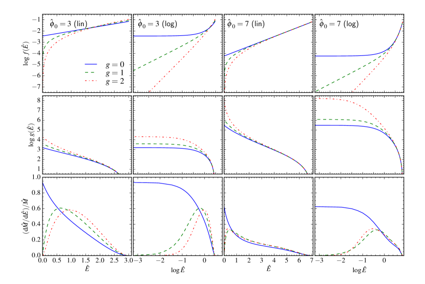
In the first and third columns (linear $x$-scale), we recognize the exponential behaviour of $f(\hat{E})$ for the $g=0$ model, and the exponential behaviour at high $\hat{E}$ for $g>0$ models. From the second and fourth column, we see that at low $\hat{E}$, the DF scales as $f(\hat{E})\propto\hat{E}^{g}$, which corresponds to the regime where the models behave as polytropes. From Fig. 2 it is also evident that when $\hat{E}\simeq\hat{\phi}_{0}$, the model behaviour is independent of $g$.

From the differential energy distribution, we see that only for $g=0$ there is a non-zero mass at $\hat{E}=0$. For models with $g>0$, the truncation is such that $f(\hat{E}=0)={\rm d}\hat{M}/{\rm d}\hat{E}\left|{}_{\hat{E}=0}\right.=0$. These models give rise to more realistic looking density profiles, but in real GCs the number of particles with the escape energy is not zero (Baumgardt, 2001), because of the gradual scattering of particles over the critical energy for escape by two-body relaxation, and because of the finite time for stars to escape from the Jacobi surface imposed by the galactic tidal field (Fukushige & Heggie, 2000).

3.1.3 Finite and infinite models

As discussed in Section 2.1.5, there are no models with finite extent if $g\geq 3.5$. GV14 showed that the maximum value $g_{\rm max}$ to get models with a finite extent depends on $\hat{\phi}_{0}$, and $g_{\rm max}=3.5$ holds in the limit of $\hat{\phi}_{0}\rightarrow 0$. GV14 show that all their isotropic models are finite for $g\lesssim 2.1$.

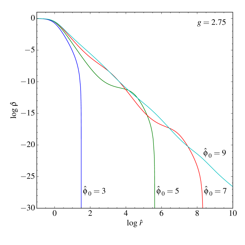
We note that there is a class of isotropic models that are finite in extent, but are not relevant to star clusters, and that are not discussed in GV14. This is illustrated in Fig. 3, where we show density profiles for models with different $\hat{\phi}_{0}$ and $g=2.75$. The model with $\hat{\phi}_{0}=3$ converges to a finite $\hat{r}_{\rm t}$ and has a density profile comparable in shape to the ones shown in Fig. 1. The model with $\hat{\phi}_{0}=9$ is infinite in extent, and only plotted up to $\log\,\hat{r}=10$. The models with $\hat{\phi}_{0}=5$ and $\hat{\phi}_{0}=7$ are finite, but show a sharp upturn in the density profile at large radii, which causes them to have a lot of mass in the envelope, but little energy, which makes these models inapplicable to real stellar systems. Their extreme density contrast between the core and the extended halo makes these models perhaps applicable to red giant stars (see the density profiles for red giants in Passy et al., 2012). To quantify the boundary between models with, and without the core-halo structure, we compute the ratio of the dimensionless virial radius $\hat{r}_{\rm v}=-G\hat{M}^{2}/(2\hat{U})$ over $\hat{r}_{\rm h}$ for a grid of models with $0\leq\hat{\phi}_{0}\leq 20$ and $0\leq g\leq 3.5$, and we show the result as contours in Fig. 4. We find that for a given $g(\hat{\phi}_{0})$, when increasing $\hat{\phi}_{0}(g)$, the change in $\hat{r}_{\rm v}/\hat{r}_{\rm h}$ is large and abrupt once the models develop the core-halo structure. We identify the value of $\hat{r}_{\rm v}/\hat{r}_{\rm h}\simeq 0.64$ as the one separating the two classes of models. In the remaining discussion, we only consider models with $\hat{r}_{\rm v}>0.64\hat{r}_{\rm h}$.

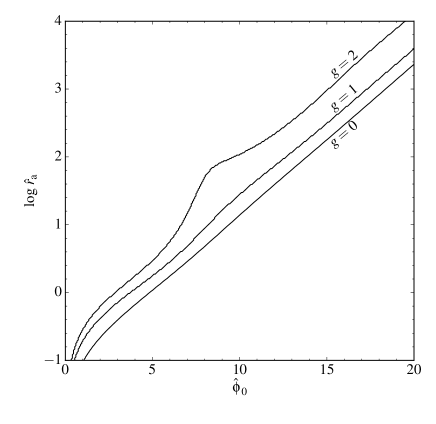
When considering anisotropic models, we find that for each $\hat{\phi}$ and $g$, there is a minimum value of $\hat{r}_{\rm a}$ that can be used to obtain a model that has a finite extent. We note that models with infinite extent can have a finite total mass, but because we envision an application of these models to tidally limited systems we do not consider them here. In Fig. 5, we show the minimum $\hat{r}_{\rm a}$ for which models are finite in extent. The lines show, as a function of $\hat{\phi}_{0}$, and for different $g$, the values of $\hat{r}_{\rm a}$ that are needed to get $\hat{r}_{\rm t}=10^{7}$. Note that this minimum for $\hat{r}_{\rm a}$ goes up approximately exponentially with $\hat{\phi}_{0}$, and also increases with $g$.

Figure 3: Density profiles for isotropic models with truncation parameter $g=2.75$. Models with $\hat{\phi}_{0}=3$, $5$, and $7$ (blue, green, and red line, respectively) have a finite truncation radius, but only the model with $\hat{\phi}_{0}=3$ is relevant when describing GCs; the model with $\hat{\phi}_{0}=9$ (light blue line) is infinite in extent.

Figure 4: Ratio of dimensionless virial radius to half-mass radius, $\hat{r}_{\rm v}/\hat{r}_{\rm h}$, for models with different $\hat{\phi}_{0}$ and $g$. We consider models with $\hat{r}_{\rm v}/\hat{r}_{\rm h}\geq 0.64$ as relevant to describe star clusters. Models that have an infinite $\hat{r}_{\rm t}$ are plotted as $\hat{r}_{\rm v}/\hat{r}_{\rm h}=0$ (i.e. they correspond to the white region in the plot).

Figure 5: Minimum $\hat{r}_{\rm a}$ for finite sized models, for different $\hat{\phi}_{0}$ and $g$.

3.1.4 Entropy

King (1966) suggested that in the process of core collapse, clusters evolve along a sequence of models with increasing central concentration. He also noted that his models are probably not able to describe the late stages of core collapse, because for large central concentration the variation in energy due to a change in the central concentration occurs in the envelope, and not in the core. Further support for this idea comes from Lynden-Bell & Wood (1968), who showed that a maximum in entropy occurs at $\hat{\phi}_{0}\simeq 9$ for both Woolley and King models at constant mass and energy. The entropy of a self-gravitating system is obtained from the DF as

$$S=-\int{\rm d}^{3}r\,{\rm d}^{3}v\,f\ln f\ .$$ (34)

Because two-body encounters continuously increase the total entropy of the system, we do not expect King models to be able to describe a system in the late stages of core collapse (i.e. $\hat{\phi}_{0}\gtrsim 9$). This was confirmed by Fokker-Planck models of isolated star clusters going into core collapse (Cohn, 1980), for which the entropy increase follows that of King models with increasing central concentration, up to a value of $\hat{\phi}_{0}\simeq 9$, but then it continues to rise during the gravothermal catastrophe. Cohn concluded that in this regime, the isotropic King models are not able to describe the entropy evolution in his simulations.

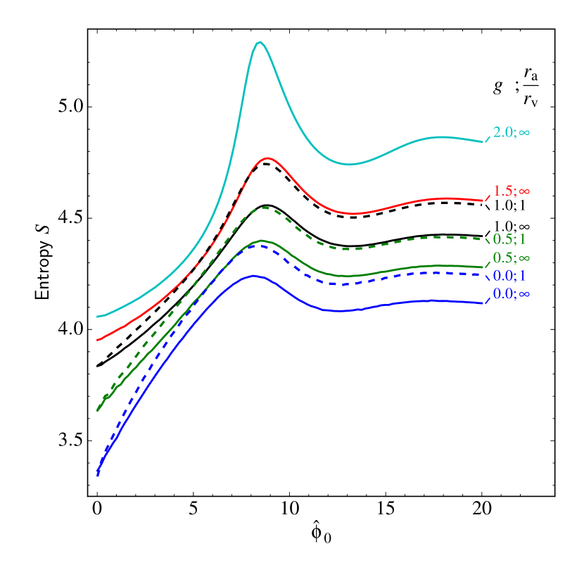
In Fig. 6, we show the entropy $S$, computed as in equation (34), for the isotropic King models (black solid line), which shows a maximum at $\hat{\phi}_{0}\simeq 9$. We also show the entropy curves for different values of $g$, and for selected anisotropic models. All models are scaled to the same $M$ and total energy $E_{\rm tot}$, in the conventional Hénon $N$-body units: $G=M=-4E_{\rm tot}=1$ (Hénon, 1971). For $0\lesssim\hat{\phi}_{0}\lesssim 1$, the anisotropic models are similar to their corresponding isotropic models, and therefore they have similar entropy. From this plot it is apparent that evolution at constant mass and energy, and with increasing entropy is possible beyond $\hat{\phi}\gtrsim 9$ if $g$ is increased, and/or $r_{\rm a}$ is decreased (i.e. including more anisotropy). A local maximum in entropy is seen near $\hat{\phi}_{0}\simeq 17$. Similar oscillating behaviour of the entropy was found for isothermal models in a non-conducting sphere and we refer to Lynden-Bell & Wood (1968) and Padmanabhan (1989) for detailed discussions. A study of equilibria in lowered isothermal models of the Woolley and King-type can be found in Katz et al. (1978); for a discussion on the evolutionary sequence of quasi-equilibrium states in $N$-body systems we refer to Taruya & Sakagami (2005). It would be of interest to compare the models discussed here to the phase-space density of particles in an $N$-body system undergoing core collapse.

Figure 6: Entropy curves for isotropic and anisotropic models with different truncation prescriptions (i.e. different values of $g$). All models are scaled to the same mass and energy. The anisotropic models are shown as dashed lines and for these models we used $r_{\rm a}=r_{\rm v}$. For $g\geq 1.5$ the anisotropic models are not finite for all $\hat{\phi}_{0}$, and the corresponding curves are therefore not plotted. This figure shows that the entropy can be increased by increasing $g$, and/or by decreasing $r_{\rm a}$.

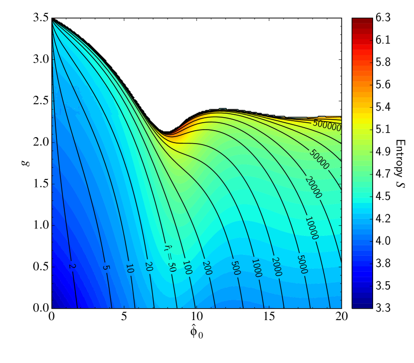
In Fig. 7, we illustrate the dependence of the entropy on $g$ and $\hat{\phi}_{0}$ for isotropic models. For a model with $g=1$ and a low concentration, the entropy can be increased by moving to the right in this diagram, and near $\hat{\phi}_{0}\simeq 9$ the entropy can be increased by increasing $g$.

Figure 7: Entropy contours for isotropic models, all scaled to $G=M=-4E_{\rm tot}=1$, with different $\hat{\phi}_{0}$ and $g$. Contours of constant $\hat{r}_{\rm t}$ are shown as black lines. Moving to the right at constant $g$ leads to an increase of entropy up to $\hat{\phi}_{0}\simeq 9$ (Lynden-Bell & Wood, 1968; Cohn, 1980). The entropy can grow further by increasing $g$ at constant $\hat{\phi}_{0}\simeq 9$. The maximum entropy is found near $\hat{\phi}_{0}\simeq 9$ and $g\simeq 2.2$.

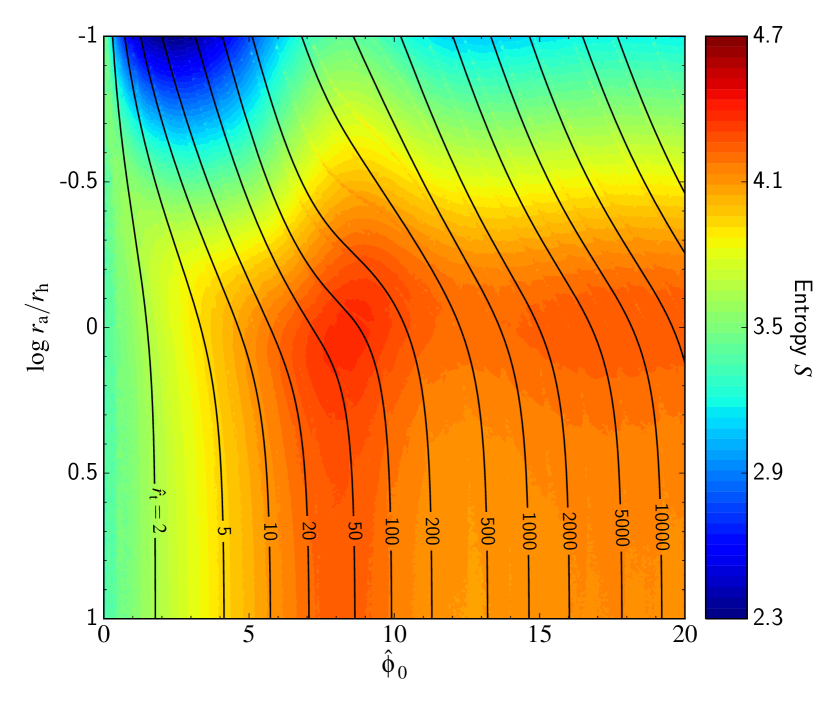
In Fig. 8, we show the dependence of entropy on anisotropy, expressed here in terms of $r_{\rm a}/r_{\rm h}$, for models with $g=0$. We see that for constant $r_{\rm a}/r_{\rm h}\gtrsim 1$, the entropy can increase by increasing $\hat{\phi}_{0}$, up to about $\hat{\phi}_{0}\simeq 9$ (this was also found by Magliocchetti et al., 1998, in a study of anisotropic Woolley, King and Wilson models). The entropy can be increased further by decreasing the anisotropy radius. A maximum is found near $\hat{\phi}_{0}\simeq 9$ and $r_{\rm a}\simeq r_{\rm h}$.

Figure 8: Entropy for models, all scaled to $G=M=-4E_{\rm tot}=1$, with $g=0$ and different concentrations and different amounts of anisotropy, quantified here in terms of $r_{\rm a}/r_{\rm h}$. Contours of constant $\hat{r}_{\rm t}$ are shown as black lines. A maximum in entropy is found at $\hat{\phi}_{0}\simeq 9$ and $r_{\rm a}\simeq r_{\rm h}$.

3.2 multimass models

Multimass models with $N_{\rm comp}$ mass bins require, in addition to the parameters of the single-mass models, $2N_{\rm comp}+2$ parameters (Section 2.2). There is, therefore, a large variety of models that can be considered, and many properties that we can chose from to illustrate the behaviour of these models. We decide to focus on two properties that highlight important features of these multimass models in relation to mass segregation. In a follow-up study (Peuten et al., in preparation) we present a detailed comparison between the multimass models and $N$-body simulations of clusters with different mass functions.

3.2.1 The role of $\delta$

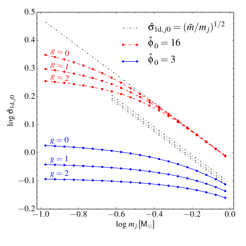
In Fig. 9 we show the dimensionless central velocity dispersion of each mass component, $\hat{\sigma}_{{\rm 1d},j0}$, as a function of its mass $m_{j}$ for isotropic, 20-component models with different $\hat{\phi}_{0}$ and $g$. The mass bins are logarithmically spaced between $0.1\,\mbox{M}_{\rm\odot}$ and $1\,\mbox{M}_{\rm\odot}$ (note that the units are not important, because the model behaviour depends only on the dimensionless values $m_{j}/\bar{m}$), and $M_{j}\propto m_{j}^{0.7}$, which corresponds to a power-law mass function ${\rm d}N/{\rm d}m_{j}\propto m_{j}^{-1.3}$ (i.e. a GC-like mass function). The mass segregation parameter was set to $\delta=1/2$ (for the definition of $\delta$, see equation 24).

Despite the fact that $m_{j}s_{j}^{2}$ is constant for all mass bins, there is no equipartition between the different mass species, i.e. $\sigma_{{\rm 1d},j0}$ does not scale as $m_{j}^{-1/2}$ for the different mass components. This is because only in the limit of infinite central concentration $\hat{\phi}_{0}\rightarrow\infty$, $s_{j}=\sigma_{{\rm 1d},j0}$, but for realistic values of $\hat{\phi}_{0}$, the ratio $\sigma_{{\rm 1d},j0}/s_{j}<1$. Because the central potential for the lower mass components is smaller than the global $\hat{\phi}_{0}$ that defines the model, the truncation in energies reduces $\sigma_{{\rm 1d},j0}$ more for low-mass components (Merritt, 1981; Miocchi, 2006). This is illustrated by the $\hat{\phi}_{0}=16$ model in Fig. 9, for which a constant $m_{j}\sigma_{{\rm 1d},j0}^{2}$ only holds for the most massive bins.

Trenti & van der Marel (2013) recently observed very similar trends between $\sigma_{{\rm 1d},j0}$ and $m_{j}$ in $N$-body models of GCs (see their fig. 1) as those shown in Fig. 9. They concluded that modelling techniques that assume equipartition, such as multimass Michie-King models, are ‘approximate at best’. We stress that multimass models that are widely used in literature, i.e. those with $\delta=1/2$ (Da Costa & Freeman, 1976; Gunn & Griffin, 1979), are not in a state of equipartition, as is illustrated in Fig. 9 and has been stated previously (Merritt, 1981; Miocchi, 2006). In fact, from a comparison of the model behaviour in Fig. 9 and the $N$-body models of Trenti and van der Marel we conclude that the most commonly chosen flavour of multimass models (i.e. King models with $\delta=1/2$) do a good job in reproducing the degree of mass segregation in evolved stellar system (see also Sollima et al., 2015).

Figure 9: Dimensionless central velocity dispersion for each mass component of multimass models with a power-law mass function, and different $\hat{\phi}_{0}$ and $g$. The value of the mass segregation parameter is $\delta=1/2$. Equipartition in energy is only reached for large values of $m_{j}$ for the model with $\hat{\phi}_{0}=16$. The dash-dotted lines show the velocity dispersion each of the models would have in the case of equipartition.

3.2.2 The role of $\eta$

In Fig. 10, we illustrate the effect of the parameter $\eta$ that sets the anisotropy radius of the different mass components (for the definition of $\eta$ see equation 25). We show the anisotropy profiles for three-component models with $m_{j}=[0.2,0.4,0.8]$, and the same mass function as before (i.e. $M_{j}\propto m_{j}^{0.7}$), and for different values of $\eta$. All models have $\hat{\phi}_{0}=9$, $g=1.5$, $\delta=1/2$ and $\hat{r}_{\rm a}=20$.

In the multimass models used in the literature $\eta$ is implicitly assumed to be $0$. From Fig. 10 we can see that this implies that the $\beta$ profile of the high-mass stars rises to larger values. It is tempting to interpret this as that massive stars are on more radial orbits. However, the more massive stars are also more centrally concentrated, where the velocity distribution is more isotropic. To quantify the importance of this effect, we show in each panel the values of the parameter $\kappa_{j}$ for each mass component (equation 33). From this we can see that in fact for the $\eta=0$ models the intermediate mass component is the most anisotropic. The relation between $\beta_{j}$ and $\kappa_{j}$ depends on the mass function, $\hat{\phi}_{0}$, and $g$ and this is therefore not a general property of $\eta=0$ models.

We note that for $\eta=\delta=1/2$ the $\beta_{j}$ profiles are nearly mass independent. Again, this does not mean that the kinetic energy in radial orbits relative to that in tangential orbits is constant, as can be seen from the values of $\kappa_{j}$. When considering a value of $\eta>1/2$ we observe that the component for which $\beta_{j}$ assumes the largest values is the least massive one.

Figure 10: Anisotropy profiles for three-component models ($m_{j}=[0.2,0.4,0.8]$) with different values for the anisotropy parameter $\eta$, that sets the anisotropy radius of the individual components as a function of their mass. All models have $\hat{\phi}_{0}=9$, $g=1.5$, $\delta=1/2$ and $\hat{r}_{\rm a}=20$. The values of $\kappa_{j}$ are shown for each component in the individual panels.

4 The limepy code

4.1 General implementation

We introduce a python-based code that solves the models and allows the user to compute some useful quantities from the DF. The code is called Lowered Isothermal Model Explorer in PYthon (limepy), and is available from: https://github.com/mgieles/limepy.

One of the main features of the code is its flexibility: the user can easily solve isotropic or anisotropic models, and include one or more mass components. The type of model to calculate is determined by the input parameters:

1. the dimensionless central potential $\hat{\phi}_{0}$;

2. the truncation parameter $g$;

3. the anisotropy radius $\hat{r}_{\rm a}$ (for anisotropic models);

4. two arrays $m_{j}$, $M_{j}$ and $\delta$ and $\eta$ (for multimass models).

By default, the model is solved in the dimensionless units described in Section 2.1.2. There we pointed out that the scales of the models are set by $A$ and $s$, which correspond to a mass density (in six-dimensional phase space) and a velocity scale. These two scales, combined with the gravitational constant $G$ then define the radial scale. To allow a user to scale a model to physical units, we decided to use the mass and radial scale as input, and from this the velocity scale is computed internally. The reason for this is that we foresee that an important application of the code is to recover the GC mass and radius from a comparison of the models to data. It is possible to scale the model to physical units by specifying $M$ in $\mbox{M}_{\rm\odot}$ and a radial scale (either $r_{\rm v}$ or $r_{\rm h}$) in ${\rm pc}$. The resulting unit of velocity is then ${\rm km}\,{\rm s}^{-1}$, with $G=0.004302\,{\rm pc}\,({\rm km}\,{\rm s}^{-1})^{2}/\mbox{M}_{\rm\odot}$. Alternative units, such as the Hénon units $G=r_{\rm v}=M=1$ (Hénon, 1971), can be considered by redefining the scales. After solving the model, the values of all typical radii are available: the King radius $r_{\rm s}$, the half-mass radius $r_{\rm h}$, the truncation radius $r_{\rm t}$, the anisotropy radius $r_{\rm a}$, and the virial radius $r_{\rm v}$.

The code solves Poisson’s equation with the ‘dopri5’ integrator (Hairer, Nørsett & Wanner, 1993), which is a Runge-Kutta integrator with adaptive step-size to calculate fourth and fifth order accurate solutions. It is supplied by the scipy sub-package integrate. The relative and absolute accuracy parameters are chosen as a compromise between speed and accuracy and can be adjusted by the user. The basic version of the code allows us to obtain, as a result of this integration, only the potential as a function of radius. The full model solution contains, in addition to the potential, the density, the radial and tangential components of the velocity dispersion, the global velocity dispersion profile, and the anisotropy profile (equation 32). It is possible to use the potential calculated in this way to compute the value of the DF as a function of input $E$ (isotropic models), or $E$ and $J$ (anisotropic models), or positions and velocities.

After solving a model, the code carries out a simple test to see whether it is in virial equilibrium: $2\hat{K}-\hat{U}=0$, where $\hat{K}$ is the dimensionless total kinetic energy (recall that $\hat{U}$ is defined to be positive, equation 31). For models that are infinite in extent, the solver stops at a large radius, the virial equilibrium assertion fails and the lack of convergence is flagged.

For multimass models the central densities of the components need to be found by iteration (Section 3.2). Gunn & Griffin (1979) proposed a recipe in which the ratios of central densities over the total density, $\alpha_{j}$, are set equal to $M_{j}/\sum_{j}M_{j}$ in the first iteration. Because for $\delta>0$ the more massive components are more centrally concentrated, the amount of mass in these components is underestimated in the first iteration, while the mass in low-mass stars is overestimated. After each iteration, $\alpha_{j}$ is multiplied by the ratio of $M_{j}/M_{j}^{\prime}$, where $M_{j}^{\prime}$ is the array of masses obtained in the previous step, and then normalized again. This is repeated until convergence. However, we found that for models with low $\hat{\phi}_{0}$ and a wide mass spectrum the mass function does not always converge with this method. We found that multiplying $\alpha_{j}$ by $\sqrt{M_{j}/M_{j}^{\prime}}$, instead, is more reliable and results in a similar number of iterations for models that do converge with the method proposed by Gunn and Griffin.

Solutions are not numerically stable when considering large values of the arguments of the hypergeometric functions. To stabilize the calculations, we adopt the asymptotic behaviour of the hypergeometric function ${{}_{1}}F_{1}(1,b,-x)$ and ${{}_{1}}F_{1}(2,b,-x)$ for $x\geq 700$ (see equations 118 and 119). For multimass models with a wide mass spectrum (e.g. when stellar mass black holes are considered in addition to the stellar mass function), the central potential of the massive component can be too large for the computation of $\mathcal{I}^{\rho}(\mu^{2\delta}\hat{\phi},\hat{r})$ (see equation 29) in the first iteration. We therefore use the approximation $\hat{\rho}_{j}=\exp[\mu^{2\delta}(\hat{\phi}-\hat{\phi}_{0})]$ if $\mu^{2\delta}\hat{\phi}>700$.

4.2 Model properties in projection

In order to compare the models to observations of GCs, it is necessary to compute the model properties in projection. For a spherically symmetric system, it is straightforward to compute the projected properties as a function of the projected radial coordinate $R$ (for a more detailed discussion, see for example Binney & Tremaine, 1987).

The projected surface mass density is found from the intrinsic mass density as

$$\Sigma(R)=2\int_{0}^{r_{\rm t}}{\rm d}z\,\rho(r),$$ (35)

where $r^{2}=R^{2}+z^{2}$, and $z$ is along the direction of the line-of-sight. The velocity dispersion along the line of sight is given by the following integral

$$\sigma_{\rm LOS}^{2}(R)=\frac{2}{\Sigma(R)}\int_{0}^{r_{\rm t}}{\rm d}z\,\rho(r)\sigma_{z}^{2}(r),$$ (36)

where $\sigma_{z}^{2}$ is the contribution of the velocity dispersion tensor to the $z$-direction. For isotropic models, $\sigma_{z}^{2}=\sigma^{2}/3$. For anisotropic models, it is possible to calculate

$$\sigma_{z}^{2}(r)=\sigma_{\rm r}^{2}\cos^{2}\xi+\sigma_{\theta}^{2}\sin^{2}\xi,$$ (37)

where $\sin\xi=R/r$. We recall that, for the anisotropic models considered here, $\sigma_{\theta}^{2}=\sigma_{\varphi}^{2}=\sigma_{\rm t}^{2}/2$. The component $\sigma_{\varphi}^{2}$ does not contribute to $\sigma_{z}^{2}$, because it is always perpendicular to the line of sight. We can use the anisotropy profile $\beta$ (see equation 32) to rewrite equation (37) as

$$\sigma_{z}^{2}(r)=\sigma_{\rm r}^{2}\left[1-\beta(r)\frac{R^{2}}{r^{2}}\right].$$ (38)

The quantity $\sigma_{\rm LOS}(R)$ is useful when comparing the models to the velocity dispersion profiles that are calculated from radial (i.e. line-of-sight) velocities. Now that proper motions data are becoming available for an increasing number of GCs (Bellini et al., 2014), it is also interesting to compare the velocity dispersion components that can be measured on the plane of the sky with those calculated from the models. This comparison is particularly important because it is a direct way to detect the presence of anisotropy in the systems. We calculate, therefore, the radial and tangential projected components of the velocity dispersion as

$$\sigma_{\rm R}^{2}(R) =\frac{2}{\Sigma(R)}\int_{0}^{r_{\rm t}}{\rm d}z\,\rho(r)\sigma_{\rm S}^{2}(r),$$ (39)

$$\sigma_{\rm T}^{2}(R) =\frac{2}{\Sigma(R)}\int_{0}^{r_{\rm t}}{\rm d}z\,\rho(r)\sigma_{\rm\varphi}^{2}(r),$$ (40)

where $\sigma_{\rm S}^{2}$ is given by

$$\sigma_{\rm S}^{2}(r)=\sigma_{\rm r}^{2}\left[1-\beta(r)\left(\frac{1-R^{2}}{r^{2}}\right)\right].$$ (41)

In the case of multimass models, the projected quantities introduced above are calculated separately for each mass component, by replacing every quantity in the equations above with the respective $j$th profile.

4.3 Generating discrete samples from the DF

A separate sampling routine limepy.sample is provided that generates discrete samples from the models. The routine takes a python object containing a model as input and the number of points $N$ that need to be sampled. In the case of a multimass models the input $N$ is ignored and computed from the total mass $M$ and the pair $m_{j},M_{j}$. Radial positions are sampled by generating numbers between 0 and 1 and interpolating the corresponding $r$ values from the (normalized) cumulative mass profile(s).

To obtain velocities, we first sample values of $x$, where $x=\hat{k}^{3/2}=(\hat{v}^{2}/2)^{3/2}$. The probability density function (PDF) for $x$ can be written as

$$P(x)=\frac{F(\hat{p}x^{1/3})}{\hat{p}x^{1/3}}E_{\gamma}(g,\hat{\phi}(\hat{r})-x^{2/3}),$$ (42)

where $\hat{p}=\hat{r}/\hat{r}_{\rm a}$. The function $P(x)$ has a maximum at $x=0$, and declines monotonically to 0 at $x=\hat{\phi}(\hat{r})^{3/2}$. These properties make it easier to efficiently sample values for $x$ from $P(x)$, than sampling values of $v$ from $v^{2}f(r,v)$. To make the rejection sampling more efficient, we adapt a supremum function $F(x)$, which consists of 10 segments between 11 values $x_{i}$ which are linearly spaced between $0$ and $\hat{\phi}(\hat{r})^{3/2}$, and for each segment $x_{i}<x<x_{i+1}$, $F_{i}(x)=P(x_{i})$. We then sample values from the function $F(x)$, reject the points that are above $P(x)$ and resample the rejected points until all points are accepted. Typically, a handful of iterations are needed.

For anisotropic models we also need to sample angles $\theta$. We do this by sampling values for $t=\cos\theta$. From the DF it follows that the PDF for $t$ is

$$P(t)=\exp\left[\hat{p}^{2}\hat{k}(t^{2}-1)\right].$$ (43)

By integrating equation (43) we find that the cumulative DF is the imaginary error function. This function cannot be inverted analytically, hence the values for $t$ need to be found by numerically inverting this function, which can be done accurately with built-in scipy routines.

When values for $r,v_{\rm t}$ and $v_{\rm r}$ are obtained, these are converted to Cartesian coordinates by generating three additional random angles.

5 Conclusions and discussion

In this study we present a family of lowered isothermal models, with the ability to consider multiple mass components and a variable amount of radially biased pressure anisotropy. The models extend the single-mass family of isotropic models recently developed by GV14. The new additions we propose here make the models ideally suited to be compared to data of resolved GCs.

The models are characterized by an isothermal and isotropic core, and a polytropic halo. The shape of the halo is set by the truncation parameter $g$, that controls the sharpness of the energy truncation, i.e. the prescription of lowering the isothermal model. For integer values of $g$, several well-known isotropic models are recovered: for $g=0$ we recover the Woolley (1954) models, for $g=1$ the Michie (1963), or King (1966) models and $g=2$ corresponds to the non-rotating, isotropic Wilson (1975) models. The DF proposed by GV14, with the introduction of the continuous parameter $g$ to determine the truncation, allows us to consider models in between these models. The advantage of this prescription for the truncation is that it is now possible to control the sharpness of the truncation by means of a parameter.

We present Lowered Isothermal Model Explorer in PYthon (limepy), a python-based code that solves the models, and computes observable quantities such as the density and velocity dispersion profile in projection. In addition, the code can be used to draw random positions and velocities from the DF, which can be used to generate initial conditions for numerical simulations.

It is interesting to discuss possible extensions of, and improvements to the models. One obvious pitfall is that the tidal field is not included in a self-consistent way. To quantify the effect of the omission of the tidal field, we can consider the specific energy $E$ at $r_{\rm t}$. In our models $E(r_{\rm t})=\phi(r_{\rm t})=-GM/r_{\rm t}$, whilst inclusion of the tidal terms would give (for a cluster on a circular orbit, in a reference frame corotating with the galactic orbit) a specific Jacobi energy of $E_{\rm J}(r_{\rm t})=-(3/2)GM/r_{\rm t}$. Therefore, the properties of stars near the critical energy for escape are described only approximately by these models, because in this energy range the galactic tidal potential is of comparable importance as the cluster potential. Another simplification of the models is that the galactic tidal potential is triaxial, whilst our models are spherical. Both of these points could be improved upon by including a galactic tidal potential in the solution of Poisson’s equation, following the methods described by Heggie & Ramamani (1995) or Bertin & Varri (2008), Varri & Bertin (2009).

The models do not include a prescription for rotation, which can be an important factor to take into account when describing real GCs (e.g. Bellazzini et al., 2012). Self-consistent models with realistic rotation curves exist (Varri & Bertin, 2012) and have been successful in describing the rotational properties of several Galactic GCs (Bianchini et al., 2013). It is feasible to include rotation in the models presented in this paper, for example, in the way it is done in the Wilson (1975) model, by multiplying the DF in equation (1) by a $J_{\rm z}$ dependent exponential term. Including the rotation, and a description of the galactic tidal field, would make the models more realistic and, therefore, a worthwhile exercise for future studies.

Lastly, we note that our models could be useful in modelling nuclear star clusters. Despite the fact that these systems are not tidally truncated in the same way as clusters on an orbit around the galaxy centre, their profiles are well described by lowered isothermal models (e.g. Georgiev & Böker, 2014). For a general application to nuclear star clusters, it is desirable to include the effect of the presence of a black hole in the centre, which generates a point-mass potential. Miocchi (2010) provided a method to self-consistently solve King models with an external point-mass potential: this recipe could be used to include the effect of a massive black hole in the models presented here, to make them more versatile in describing nuclear star clusters.

The aim of this project was to introduce models that can be used to describe the phase-space density of stars in tidally limited, mass-segregated star clusters, in any stage of their life-cycle. At early stage, GCs are dense with respect to their tidal density (e.g. Alexander & Gieles, 2013) and at the present day about half of the GCs is still much denser than their tidal density (Baumgardt et al., 2010; Gieles et al., 2011). These GCs ought to have a population of stars with radial orbits in their envelopes, either as a left-over of the violent relaxation process during their formation (Lynden-Bell, 1967), and/or because of two-body ejections from the core (Spitzer & Shapiro, 1972). In this phase we expect models with high values of $g$, and small $r_{\rm a}$ to describe GCs well. These models can thus describe GCs with large Jacobi radii, relative to $r_{\rm h}$. This applies to a large fraction of the Milky Way GC population, and these objects are beyond the reach of King models (Baumgardt et al., 2010). In later stages of evolution, GCs will be more tidally limited, and isotropic, hence we expect $g$ to reduce and $r_{\rm a}$ to increase during the evolution (up to a value that practically corresponds to having isotropic models). Capturing these variations in GCs properties with continuous parameters has the advantage that these parameters can be inferred from data. This avoids the need of a comparison of goodness-of-fit parameters of different models.

When only surface brightness data are available, it is challenging to distinguish between models with different truncation flavours and pressure anisotropy, because their role has an impact mostly on the low-density outer parts, far from the centre of the cluster, where foreground stars and background stars are dominating. The addition of kinematical data of stars in the outer region of GCs greatly aids in discriminating between models, but this is challenging at present. Precise proper motions ($\lesssim 1\,{\rm km}\,{\rm s}^{-1}$) can be obtained with the Hubble Space Telescope (HST; e.g. McLaughlin et al., 2006; Watkins et al., 2015), but the field of view of HST limits observations to the central parts of Milky Way GCs. Radial velocity measurements of stars in the outer parts of GCs are expensive because of the contamination of non-member stars (Da Costa, 2012). The upcoming data of the ESA-Gaia mission will improve this situation: the availability of all-sky proper motions and photometry measurements will facilitate membership selection, and for several nearby GC the proper motions will be of sufficient quality that they can be used for dynamical modelling and to unveil the properties of the hidden low-energy stars (An et al., 2012; Pancino et al., 2013; Sollima et al., 2015). The models presented in this paper allow for higher level of inference of physical properties of GCs from these upcoming data.

In two forthcoming studies we will compare the family of models to a series of direct $N$-body simulations of the long term evolution of single-mass star clusters (Zocchi et al., 2016) and multimass clusters (Peuten et al., in preparation) evolving in a tidal field.

Appendix A Derivations

The DF introduced in equation (1) can be expressed as a function of the dimensionless quantities $\hat{\phi}$, $\hat{k}$ and $\hat{p}$ defined in Sections 2.1.2 and 2.1.4 as

$$f=A\exp\left(-\hat{k}\hat{p}^{2}\sin^{2}\theta\right)E_{\gamma}\left(g,\hat{\phi}-\hat{k}\right).$$ (44)

We want to calculate, for these models, the density and velocity dispersion components. We recall that these quantities can be obtained from the DF in the following way:

$$\rho =\int{\rm d}^{3}v\,f,$$ (45)

$$\sigma^{2}_{i} =\frac{1}{\rho}\int{\rm d}^{3}v\,fv^{2}_{i},$$ (46)

where the subscript $i$ denotes the $i$-th component of the velocity vector. To carry out these integrals of the DF in the three-dimensional velocity volume we can use the dimensionless variable $\hat{k}$ and the variable $t=\cos\theta$

$${\rm d}^{3}v={\rm d}v{\rm d}\theta{\rm d}\varphi\,v^{2}\sin\theta=-{\rm d}\hat{k}{\rm d}t{\rm d}\varphi\,\sqrt{\hat{k}}(2s^{2})^{3/2}.$$ (47)

In calculating the relevant quantities mentioned above, we encounter the following integrals with respect to the variable $t$

$$\int_{0}^{1}{\rm d}t\,\exp\left[-\hat{k}\hat{p}^{2}(1-t^{2})\right]=\frac{F\left(\sqrt{\hat{k}}\hat{p}\right)}{\sqrt{\hat{k}}\hat{p}},$$ (48)

$$\int_{0}^{1}{\rm d}t\,t^{2}\exp\left[-\hat{k}\hat{p}^{2}(1-t^{2})\right]=\frac{1}{2\hat{k}\hat{p}^{2}}-\frac{F\left(\sqrt{\hat{k}}\hat{p}\right)}{2(\sqrt{\hat{k}}\hat{p})^{3}},$$ (49)

where $F(x)$ is the Dawson integral, whose properties are presented in Section D.3. We use the above results to proceed and derive the density and velocity components.

A.1 Density profile

The density is calculated as

$$\rho =\int{\rm d}^{3}v\,f$$

$$=\frac{\tilde{A}}{\sqrt{\pi}}\int_{0}^{\hat{\phi}}{\rm d}\hat{k}\,\int_{0}^{1}{\rm d}t\,\hat{k}^{1/2}\exp\left[\hat{k}\hat{p}^{2}(t^{2}-1)\right]E_{\gamma}\left(g,\hat{\phi}-\hat{k}\right)$$

$$=\tilde{A}\frac{2}{\sqrt{\pi}}\int_{0}^{\hat{\phi}}{\rm d}\hat{k}\,\frac{F\left(\sqrt{\hat{k}}\hat{p}\right)}{\hat{p}}E_{\gamma}\left(g,\hat{\phi}-\hat{k}\right)$$

$$=\tilde{A}\mathcal{I}^{\rho},$$ (50)

where we replaced $\Gamma(3/2)$ by $\sqrt{\pi}/2$, and we introduced $\tilde{A}=A\left(2\pi s^{2}\right)^{3/2}$ and we solved the integral over $t$ as shown in equation (48). The integral $\mathcal{I}^{\rho}$ can be solved by first doing an integration by parts (by using the results in equations 104 and 109) and by then using the convolution formula of equation (105) and the recurrence relation of equation (102) in the following way:

$$\mathcal{I}^{\rho} =\frac{2}{\sqrt{\pi}}\int_{0}^{\hat{\phi}}{\rm d}\hat{k}\,E_{\gamma}\left(g,\hat{\phi}-\hat{k}\right)\frac{F\left(\sqrt{\hat{k}}\hat{p}\right)}{\hat{p}}$$ (51)

$$=\frac{2}{\sqrt{\pi}}\int_{0}^{\hat{\phi}}{\rm d}\hat{k}\,E_{\gamma}\left(g+1,\hat{\phi}-\hat{k}\right)\times\left[\frac{1}{2\sqrt{\hat{k}}}-\hat{p}F\left(\sqrt{\hat{k}}\hat{p}\right)\right]$$

$$=E_{\gamma}\left(g+\tfrac{3}{2},\hat{\phi}\right)-\hat{p}^{2}\frac{2}{\sqrt{\pi}}\int_{0}^{\hat{\phi}}{\rm d}\hat{k}\,E_{\gamma}\left(g,\hat{\phi}-\hat{k}\right)\frac{F\left(\sqrt{\hat{k}}\hat{p}\right)}{\hat{p}}$$

$$\hskip 28.45274pt+\hat{p}^{2}\frac{2}{\sqrt{\pi}}\int_{0}^{\hat{\phi}}{\rm d}\hat{k}\,\frac{\left(\hat{\phi}-\hat{k}\right)^{g}}{\Gamma(g+1)}\frac{F\left(\sqrt{\hat{k}}\hat{p}\right)}{\hat{p}}$$

$$=E_{\gamma}\left(g+\tfrac{3}{2},\hat{\phi}\right)-\hat{p}^{2}\mathcal{I}^{\rho}+\hat{p}^{2}\mathcal{I}_{F,1}.$$ (52)

The integral $\mathcal{I}_{F,1}$ can be calculated by substituting the Dawson function for its series representation (see equation 108), by changing variable to $y=\hat{k}/\hat{\phi}$, by using the Beta function of equation (106), and by recognizing the expression in equation (110)

$$\mathcal{I}_{F,1} =\frac{2}{\sqrt{\pi}}\int_{0}^{\hat{\phi}}{\rm d}\hat{k}\,\frac{\left(\hat{\phi}-\hat{k}\right)^{g}}{\Gamma(g+1)}\frac{F\left(\sqrt{\hat{k}}\hat{p}\right)}{\hat{p}}$$

$$=\frac{\hat{\phi}^{g+\frac{3}{2}}{{}_{1}}F_{1}\left(1,g+\tfrac{5}{2},-\hat{p}^{2}\hat{\phi}\right)}{\Gamma\left(g+\frac{5}{2}\right)},$$ (53)

where ${{}_{1}}F_{1}\left(a,b,x\right)$ is the confluent hypergeometric function (see Section D.4). Therefore, we can finally write the density integral as

$$\mathcal{I}^{\rho}\!=\!\frac{E_{\gamma}(g+\tfrac{3}{2},\hat{\phi})}{1+\hat{p}^{2}}+\frac{\hat{p}^{2}}{1+\hat{p}^{2}}\frac{\hat{\phi}^{g+\frac{3}{2}}{{}_{1}}F_{1}(1,g+\frac{5}{2},-\hat{p}^{2}\hat{\phi})}{\Gamma\left(g+\frac{5}{2}\right)}.$$ (54)

A.2 Velocity dispersion profiles

The velocity dispersion profile can be computed in a similar way as the density, by using again the result in equation (48)

$$\sigma^{2}\rho =\int{\rm d}^{3}v\,v^{2}f$$

$$=\frac{2\tilde{A}s^{2}}{\sqrt{\pi}}\int_{0}^{\hat{\phi}}{\rm d}\hat{k}\!\int_{0}^{1}{\rm d}t\,\exp\left[{-\hat{k}\hat{p}^{2}(1-t^{2})}\right]\hat{k}^{3/2}E_{\gamma}(g,\hat{\phi}-\hat{k})$$

$$=\frac{4\tilde{A}s^{2}}{\sqrt{\pi}}\int_{0}^{\hat{\phi}}{\rm d}\hat{k}\,\frac{F(\sqrt{\hat{k}}\hat{p})}{\hat{p}}\hat{k}E_{\gamma}(g,\hat{\phi}-\hat{k})$$

$$=\tilde{A}s^{2}\mathcal{I}^{\rho\sigma^{2}}.$$ (55)

The integral $\mathcal{I}^{\rho\sigma^{2}}$ can be solved with an integration by parts, then by using equation (105), and finally, after having used the recurrence relation of equation (102), by recognizing the presence of the integral $\mathcal{I}^{\rho}$ found when calculating the density

$$\mathcal{I}^{\rho\sigma^{2}} =\frac{4}{\sqrt{\pi}}\int_{0}^{\hat{\phi}}{\rm d}\hat{k}\,\hat{k}E_{\gamma}\left(g,\hat{\phi}-\hat{k}\right)\frac{F\left(\sqrt{\hat{k}}\hat{p}\right)}{\hat{p}}$$ (56)

$$=\frac{4}{\sqrt{\pi}}\int_{0}^{\hat{\phi}}{\rm d}\hat{k}\,E_{\gamma}\left(g+1,\hat{\phi}-\hat{k}\right)$$

$$\hskip 28.45274pt\times\left[\frac{\sqrt{\hat{k}}}{2}+\frac{F\left(\sqrt{\hat{k}}\hat{p}\right)}{\hat{p}}-\hat{k}\hat{p}^{2}\frac{F\left(\sqrt{\hat{k}}\hat{p}\right)}{\hat{p}}\right]$$

$$=E_{\gamma}\left(g+\tfrac{5}{2},\hat{\phi}\right)+2\mathcal{I}^{\rho}_{g+1}+\hat{p}^{2}\left(\mathcal{I}_{F,2}-\mathcal{I}^{\rho\sigma^{2}}\right),$$ (57)

where $\mathcal{I}^{\rho}_{g+1}=\mathcal{I}^{\rho}(g+1,\hat{p},\hat{\phi})$. We then solve the integral $\mathcal{I}_{F,2}$ in a similar way as we did for $\mathcal{I}_{F,1}$, to get

$$\mathcal{I}_{F,2} =\frac{4}{\sqrt{\pi}}\int_{0}^{\hat{\phi}}{\rm d}\hat{k}\,\hat{k}\frac{F\left(\sqrt{\hat{k}}\hat{p}\right)}{\hat{p}}\frac{\left(\hat{\phi}-\hat{k}\right)^{g}}{\Gamma(g+1)}$$

$$=\frac{\hat{\phi}^{g+\frac{5}{2}}}{\Gamma\left(g+\tfrac{7}{2}\right)}\left[{{}_{1}}F_{1}\left(1,g+\tfrac{7}{2},-\hat{p}^{2}\hat{\phi}\right)\right.$$

$$\left.+2{{}_{1}}F_{1}\left(2,g+\tfrac{7}{2},-\hat{p}^{2}\hat{\phi}\right)\right].$$ (58)

Therefore, we finally have

$$\sigma^{2}\rho =\frac{\tilde{A}s^{2}}{(\hat{p}^{2}+1)}\left\{E_{\gamma}\left(g+\tfrac{5}{2},\hat{\phi}\right)\left(\frac{3+\hat{p}^{2}}{1+\hat{p}^{2}}\right)\right.$$

$$\left.+\frac{\hat{p}^{2}\hat{\phi}^{g+\tfrac{5}{2}}}{\Gamma\left(g+\frac{7}{2}\right)}\left[2\,{{}_{1}}F_{1}\left(2,g+\tfrac{7}{2},-\hat{p}^{2}\hat{\phi}\right)\right.\right.$$

$$\left.\left.+{{}_{1}}F_{1}\left(1,g+\tfrac{7}{2},-\hat{p}^{2}\hat{\phi}\right)\left(\frac{3+\hat{p}^{2}}{1+\hat{p}^{2}}\right)\right]\right\}.$$ (59)

The radial component of the velocity dispersion is given by

$$\sigma_{\rm r}^{2}\rho =\int{\rm d}^{3}v\,(v\cos\theta)^{2}f$$

$$=\frac{2\tilde{A}s^{2}}{\sqrt{\pi}}\int_{0}^{\hat{\phi}}{\rm d}\hat{k}\,\hat{k}^{3/2}E_{\gamma}\left(g,\hat{\phi}-\hat{k}\right)\left[\frac{1}{\hat{k}\hat{p}^{2}}-\frac{F\left(\sqrt{\hat{k}}\hat{p}\right)}{(\sqrt{\hat{k}}\hat{p})^{3}}\right]$$

$$=\frac{\tilde{A}s^{2}}{\hat{p}^{2}}\left[E_{\gamma}\left(g+\tfrac{3}{2},\hat{\phi}\right)-\mathcal{I}^{\rho}\right],$$ (60)

where we solved the integral by using equations (49) and (105). We point out that we can express this quantity by means of the density integrals of the isotropic and the anisotropic case (see also equations 8 and 10 in Section 2). We finally obtain

$$\sigma_{\rm r}^{2}\rho=\tilde{A}s^{2}\left[\frac{E_{\gamma}\left(g+\tfrac{3}{2},\hat{\phi}\right)}{(1+\hat{p}^{2})}-\frac{\hat{\phi}^{g+\tfrac{3}{2}}{{}_{1}}F_{1}\left(1,g+\tfrac{5}{2},-\hat{p}^{2}\hat{\phi}\right)}{(1+\hat{p}^{2})\Gamma\left(g+\frac{5}{2}\right)}\right],$$ (61)

which, by using equations (102) and (113), can be rewritten as

$$\sigma_{\rm r}^{2}\rho=\tilde{A}s^{2}\left[\frac{E_{\gamma}\left(g+\tfrac{5}{2},\hat{\phi}\right)}{(1+\hat{p}^{2})}+\frac{\hat{p}^{2}\hat{\phi}^{g+\tfrac{5}{2}}{{}_{1}}F_{1}\left(1,g+\frac{7}{2},-\hat{p}^{2}\hat{\phi}\right)}{(1+\hat{p}^{2})\Gamma\left(g+\frac{7}{2}\right)}\right].$$ (62)

To calculate the tangential component of the velocity dispersion we solve the integral over $t$ by expressing it as the difference between equation (48) and equation (49), and we carry out an integration by parts

$$\sigma_{\rm t}^{2}\rho =\int{\rm d}^{3}v\,(v\sin\theta)^{2}f$$

$$=\frac{2\tilde{A}s^{2}}{\sqrt{\pi}}\int_{0}^{\hat{\phi}}{\rm d}\hat{k}\,\hat{k}^{3/2}E_{\gamma}\left(g,\hat{\phi}-\hat{k}\right)$$

$$\hskip 7.11317pt\times\left[\frac{2F\left(\sqrt{\hat{k}}\hat{p}\right)}{\sqrt{\hat{k}}\hat{p}}-\frac{1}{\hat{k}\hat{p}^{2}}+\frac{F\left(\sqrt{\hat{k}}\hat{p}\right)}{(\sqrt{\hat{k}}\hat{p})^{3}}\right]$$

$$=\frac{\tilde{A}s^{2}}{\hat{p}^{2}}\left[\hat{p}^{2}\mathcal{I}^{\rho\sigma^{2}}-E_{\gamma}\left(g+\tfrac{3}{2},\hat{\phi}\right)+\mathcal{I}^{\rho}\right].$$ (63)

After recognizing the integrals we solved above, we can finally write

$$\sigma_{\rm t}^{2}\rho =\frac{\tilde{A}s^{2}}{(1+\hat{p}^{2})}\left\{E_{\gamma}\left(g+\textstyle{\frac{5}{2}}\displaystyle,\hat{\phi}\right)\frac{2}{(1+\hat{p}^{2})}\right.$$

$$\left.+\,\frac{2\hat{p}^{2}\hat{\phi}^{g+\tfrac{5}{2}}}{\Gamma(g+\tfrac{7}{2})}\left[\frac{{{}_{1}}F_{1}\left(1,g+\tfrac{7}{2},-\hat{\phi}\hat{p}^{2}\right)}{(1+\hat{p}^{2})}\right.\right.$$

$$\left.\left.+\,{{}_{1}}F_{1}\left(2,g+\tfrac{7}{2},-\hat{\phi}\hat{p}^{2}\right)\right]\right\}\ .$$ (64)

Appendix B Derivations using fractional calculus

Fractional calculus is a branch of mathematics that considers real numbers for the orders of derivatives and integration. Because the integrals that need to be solved contain terms like $\hat{k}^{1/2}$ and $\hat{k}^{3/2}$, we can use semi-derivatives and semi-integrals and integration by parts to solve them. By following Bourdin & Idczak (2014), we define the left- and right-sided Riemann-Liouville fractional integrals of order $\alpha>0$ of a function $q\in L^{1}$ as

$$I^{\alpha}_{a+}q(t) =\frac{1}{\Gamma(\alpha)}\int_{a}^{t}{\rm d}x\,q(x)(t-x)^{\alpha-1},$$ (65)

$$I^{\alpha}_{b-}q(t) =\frac{1}{\Gamma(\alpha)}\int_{t}^{b}{\rm d}x\,q(x)(x-t)^{\alpha-1}.$$ (66)

In the remainder of this section, we will use the result illustrated by Bourdin & Idczak (2014) in their Proposition 2 (for a proof see Samko et al., 1993)

$$\int_{a}^{b}{\rm d}t\,\left(I^{\alpha}_{a+}q_{1}\right)(t)q_{2}(t)=\int_{a}^{b}{\rm d}t\,q_{1}(t)\left(I^{\alpha}_{b-}q_{2}\right)(t).$$ (67)

B.1 Density

When considering the isotropic limit of the DF, the integral to be solved to calculate the density is:

$$\mathcal{I}^{\rho}=\frac{2}{\sqrt{\pi}}\int_{0}^{\hat{\phi}}{\rm d}\hat{k}\,\hat{k}^{1/2}E_{\gamma}\left(g,\hat{\phi}-\hat{k}\right).$$ (68)

We can use fractional calculus to solve it, by changing variable of integration (using $x=\hat{\phi}-\hat{k}$) and by considering that

$$q_{1}(x) =E_{\gamma}\left(g,x\right),$$ (69)

$$q_{2}(x) =1,$$ (70)

$$I^{1/2}_{0+}q_{1}(x) =E_{\gamma}\left(g+\tfrac{1}{2},x\right),$$ (71)

$$I^{1/2}_{\hat{\phi}-}q_{2}(x) =\frac{2(\hat{\phi}-x)^{1/2}}{\sqrt{\pi}},$$ (72)

thus obtaining

$$\mathcal{I}^{\rho} =\int_{0}^{\hat{\phi}}{\rm d}x\,E_{\gamma}(g+\tfrac{1}{2},x)=E_{\gamma}(g+\tfrac{3}{2},\hat{\phi}),$$ (73)

which was solved by using equation (104).

The density of the anisotropic models is calculated by solving the integral $\mathcal{I}^{\rho}$ introduced in equation (51). To do this, we can use the result shown in equation (67) by noticing (see equations 105 and 107) that

$$q_{1}(\hat{k}) =\exp\left(-\hat{k}\hat{p}^{2}\right),$$ (74)

$$q_{2}(\hat{k}) =E_{\gamma}\left(g,\hat{\phi}-\hat{k}\right),$$ (75)

$$I^{1/2}_{0+}q_{1}(\hat{k}) =\frac{2F(\sqrt{\hat{k}}\hat{p})}{\sqrt{\pi}\hat{p}},$$ (76)

$$I^{1/2}_{\hat{\phi}-}q_{2}(\hat{k}) =E_{\gamma}\left(g+\tfrac{1}{2},\hat{\phi}-\hat{k}\right),$$ (77)

and by rewriting the integral of equation (51) as

$$\mathcal{I}^{\rho}=\int_{0}^{\hat{\phi}}{\rm d}\hat{k}\,\exp\left(-\hat{k}\hat{p}^{2}\right)E_{\gamma}\left(g+\tfrac{1}{2},\hat{\phi}-\hat{k}\right).$$ (78)

This integral can be solved by parts, by using the expression of the derivative of the lower incomplete gamma function (equation 98) and by using equation (111) to obtain

$$\mathcal{I}^{\rho}=\frac{E_{\gamma}\left(g+\tfrac{1}{2},\hat{\phi}\right)}{1+\hat{p}^{2}}-\frac{\hat{\phi}^{g+\tfrac{1}{2}}{{}_{1}}F_{1}(1,g+\tfrac{3}{2},-\hat{\phi}\hat{p}^{2})}{(1+\hat{p}^{2})\Gamma(g+\tfrac{3}{2})}.$$ (79)

The last step can be rewritten as equation (54) by using the recurrence relations shown in equations (102) and (113).

B.2 Velocity dispersion

In the isotropic limit of the DF, the velocity dispersion is calculated by means of an integral with the same structure as the one found in equation (68). The velocity dispersion of the anisotropic models is calculated by solving the integral $\mathcal{I}^{\rho\sigma^{2}}$ introduced in equation (56). We can use the result shown in equation (67) also in this case, by considering the function $q_{1}$ introduced in equation (74), its fractional integral (equation 76), and

$$q_{2}(\hat{k}) =\hat{k}\,E_{\gamma}\left(g,\hat{\phi}-\hat{k}\right),$$ (80)

$$I^{1/2}_{\hat{\phi}-}q_{2}(\hat{k}) =\frac{1}{2}E_{\gamma}\left(g+\tfrac{3}{2},\hat{\phi}-\hat{k}\right)+\hat{k}E_{\gamma}\left(g+\tfrac{1}{2},\hat{\phi}-\hat{k}\right),$$ (81)

and by rewriting the integral $\mathcal{I}^{\rho\sigma^{2}}$ as

$$\mathcal{I}^{\rho\sigma^{2}} =\int_{0}^{\hat{\phi}}{\rm d}\hat{k}\exp\left(-\hat{k}\hat{p}^{2}\right)E_{\gamma}\left(g+\tfrac{3}{2},\hat{\phi}-\hat{k}\right)$$

$$+2\int_{0}^{\hat{\phi}}{\rm d}\hat{k}\exp\left(-\hat{k}\hat{p}^{2}\right)\hat{k}E_{\gamma}\left(g+\tfrac{1}{2},\hat{\phi}-\hat{k}\right).$$ (82)

The first integral is in the same form as the one we found for the density, and the second one can be reduced to something similar with an integration by parts. By solving the integrals, we obtain:

$$\mathcal{I}^{\rho\sigma^{2}} =\frac{1}{1+\hat{p}^{2}}\left[E_{\gamma}\left(g+\tfrac{3}{2},\hat{\phi}\right)\left(\frac{3+\hat{p}^{2}}{1+\hat{p}^{2}}\right)-\frac{2\hat{\phi}^{g+\tfrac{3}{2}}}{\Gamma\left(g+\tfrac{3}{2}\right)}\right.$$

$$\left.+\frac{2\hat{\phi}^{g+\tfrac{3}{2}}{{}_{1}}F_{1}(1,g+\frac{5}{2},-\hat{\phi}\hat{p}^{2})}{\Gamma\left(g+\frac{5}{2}\right)}\left(g+\hat{p}^{2}\hat{\phi}+\frac{\hat{p}^{2}}{1+\hat{p}^{2}}\right)\right],$$ (83)

which can be rewritten as equation (59) by using the recurrence relations shown in equations (102), (112), and (113).

By inspecting equations (60) and (63), it is immediate to notice that the radial and tangential components of the velocity dispersion are calculated with integrals that can be written as a combination of those solved in this section by means of fractional calculus.

Appendix C Differential energy distribution

The differential energy distribution gives the amount of mass per units of energy (Binney & Tremaine, 1987). Here we briefly recall how to calculate it for isotropic and anisotropic systems.

For a DF that only depends on $E$, the differential energy distribution can be calculated as:

$$\frac{{\rm d}M}{{\rm d}E}\equiv f(E)\mathfrak{g}(E),$$ (84)

where $f(E)$ is the DF, and $\mathfrak{g}(E)$ is the density of states, which is the volume of phase space per unit energy and is defined as

$${\mathfrak{g}}(E)=\int{\rm d}^{3}r\,{\rm d}^{3}v\,\delta(E-H),$$ (85)

where $\delta(x)$ is the Dirac delta function. For a spherically symmetric systems, this integral can be expressed as

$$\mathfrak{g}(E)=16\pi^{2}\,\int_{0}^{r_{\rm m}(E)}{\rm d}r\,r^{2}\,\int{\rm d}v\,v^{2}\,\delta\left(\frac{1}{2}v^{2}+\phi-E\right),$$ (86)

where $r_{\rm m}(E)$ is the radius at which $\phi=E$. By changing variable (using $y=v^{2}/2$), we finally obtain

$$\mathfrak{g}(E)=16\pi^{2}\,\int_{0}^{r_{\rm m}(E)}{\rm d}r\,r^{2}\,\sqrt{2(E-\phi)},$$ (87)

and the differential energy distribution is therefore

$$\frac{{\rm d}M}{{\rm d}E}=16\pi^{2}\,f(E)\,\int_{0}^{r_{\rm m}(E)}{\rm d}r\,r^{2}\,\sqrt{2(E-\phi)}.$$ (88)

When considering anisotropic systems, for which the DF depends also on the angular momentum $J$, the differential energy distribution is obtained as

$$\frac{{\rm d}M}{{\rm d}E}=\int{\rm d}^{3}r\,{\rm d}^{3}v\,\delta(E-H)f(H,J).$$ (89)

This integral can be expressed as

$$\frac{{\rm d}M}{{\rm d}E}=8\pi^{2}\int{\rm d}r\,r^{2}\int{\rm d}v_{\rm r}\,{\rm d}v_{\rm t}\,v_{\rm t}\,\delta(E-H)f(H,J),$$ (90)

and it can then be rearranged by changing variable and introducing $J=r\,v_{\rm t}$ in the following way

$$\frac{{\rm d}M}{{\rm d}E}=8\pi^{2}\int{\rm d}r\int{\rm d}v_{\rm r}\,{\rm d}J\,J\,\delta(E-H)f(H,J).$$ (91)

The integral over $v_{\rm r}$ is solved by using the fact that

$$v_{\rm r}^{2}=2(E-\Phi)-\frac{J^{2}}{r^{2}},$$ (92)

to obtain

$$\frac{{\rm d}M}{{\rm d}E}=16\pi^{2}\,\int{\rm d}r\int{\rm d}J\,\frac{Jf(E,J)}{\sqrt{2(E-\Phi)-J^{2}/r^{2}}}.$$ (93)

By using the expression for the DF of the models presented in this paper (equation 1) we can perform the integration over $J$ in this last equation and write the differential energy distribution as a function of the part of the DF that depends on energy only, $f(E)$:

$$\frac{{\rm d}M}{{\rm d}E}=16\pi^{2}\,f(E)\,\int_{0}^{r_{\rm m}(E)}{\rm d}r\,\sqrt{2}\,r_{\rm a}s\,r\,F\left(\frac{r\sqrt{E-\phi}}{r_{\rm a}s}\right),$$ (94)

where $F(x)$ is the Dawson integral (see Appendix D.3). In the limit of $r_{\rm a}\rightarrow\infty$ this reduces to the result for the isotropic case shown in equation (88), which follows from substituting the leading term of equation (D14) in equation (C11).

Appendix D Useful properties of mathematical functions

D.1 Useful properties of the gamma functions

The gamma function of a positive integer $n$ is defined as

$$\Gamma(n)=(n-1)!,$$ (95)

while for non-integer arguments $a$, it can be written as an integral

$$\Gamma(a)=\int_{0}^{\infty}{\rm d}t\,t^{a-1}\exp(-t).$$ (96)

The lower incomplete gamma function is given by

$$\gamma(a,x)=\int_{0}^{x}{\rm d}t\,t^{a-1}\exp(-t),$$ (97)

and its derivative is

$$\frac{{\rm d}\gamma(a,x)}{{\rm d}x}=x^{a-1}\exp(-x).$$ (98)

D.2 Useful properties of the $E_{\gamma}(a,x)$ function

The exponential function $E_{\gamma}(a,x)$ is defined as

$$E_{\gamma}(a,x)=\frac{1}{\Gamma(a)}\int_{0}^{x}{\rm d}t\,t^{a-1}\exp(x-t),$$ (99)

and an alternative expression is given by means of the lower incomplete gamma function

$$E_{\gamma}(a,x)=\frac{\exp(x)\gamma(a,x)}{\Gamma(a)}.$$ (100)

The series representation of this function is

$$E_{\gamma}(a,x)=\sum_{i=0}^{\infty}\frac{x^{i+a}}{\Gamma(i+a+1)}.$$ (101)

The following recurrence relation holds

$$E_{\gamma}(a,x)=E_{\gamma}(a+1,x)+\frac{x^{a}}{\Gamma(a+1)}.$$ (102)

The derivative and the integral of $E_{\gamma}(a,x)$ are given by

$$\frac{{\rm d}E_{\gamma}(a,x)}{{\rm d}x} =E_{\gamma}(a-1,x),$$ (103)

$$\int{\rm d}x\,E_{\gamma}(a,x) =E_{\gamma}(a+1,x)+\mathrm{constant}.$$ (104)

A proof of these equations can be easily obtained by writing $E_{\gamma}(a,x)$ as in equation (100), and by considering equation (98) and the recurrence relation (equation 102). The convolution formula

$$\frac{1}{\Gamma(b)}\int_{0}^{x}{\rm d}y\,E_{\gamma}(a,x-y)y^{b-1}=E_{\gamma}(a+b,x)$$ (105)

can be obtained by using the series representation of $E_{\gamma}(a,x)$ (equation 101) and by changing variable, to express the integral with a form that allows us to recognize the Beta function:

$$B(m,n)=\int_{0}^{1}{\rm d}y\,(1-y)^{m-1}y^{n-1}=\frac{\Gamma(m)\Gamma(n)}{\Gamma(m+n)}.$$ (106)

The identity of equation (105) accounts for the fractional integration of $E_{\gamma}(a,x)$ (see equation 65).

D.3 Useful properties of the Dawson integral

The Dawson integral (sometimes called the Dawson function) is defined as

$$F(x)=\exp(-x^{2})\int_{0}^{x}{\rm d}y\exp(y^{2}).$$ (107)

It is also possible to express $F(x)$ as a sum as

$$F(x)=\sum_{i=0}^{\infty}\frac{(-1)^{i}x^{2i+1}\Gamma\left(\tfrac{3}{2}\right)}{\Gamma\left(i+\tfrac{3}{2}\right)}\ .$$ (108)

The Dawson integral is an odd function, and its derivative is

$$\frac{{\rm d}F(x)}{{\rm d}x}=1-2xF(x).$$ (109)

D.4 Useful properties of the confluent hypergeometric function

The confluent hypergeometric function is defined as

$${{}_{1}}F_{1}(a,b,x) =\displaystyle\sum_{i=0}^{\infty}\frac{\Gamma(a+i)}{\Gamma(a)}\frac{\Gamma(b)}{\Gamma(b+i)}\frac{x^{i}}{\Gamma(i+1)}.$$ (110)

It can also be defined by means of an integral, as

$${{}_{1}}F_{1}(a,b,x)=\frac{\Gamma(b)}{\Gamma(a)\Gamma(b-a)}\int_{0}^{1}{\rm d}y\,\exp(xy)y^{a-1}(1-y)^{b-a-1},$$ (111)

which holds for ${\rm Re}(b)>{\rm Re}(a)>0$. The following recurrence relations hold

$${{}_{1}}F_{1}(2,b,x) =(2-b+x)\,{{}_{1}}F_{1}(1,b,x)+b-1,$$ (112)

$$x\,{{}_{1}}F_{1}(1,b+1,x) =b\,{{}_{1}}F_{1}(1,b,x)-b.$$ (113)

We also note that this function is related to the exponential function, and for $b=a$ we have ${{}_{1}}F_{1}(a,a,x)=\exp(x)$. Another useful property of this function is that

$${{}_{1}}F_{1}(a,b,0)=1.$$ (114)

The density (equation 11) and the velocity moments (equations 15 - 17) of anisotropic models are expressed by means of the function ${{}_{1}}F_{1}(a,b,x)$ with $a=1$. When considering $a=1$ in equation (111), we obtain

$${{}_{1}}F_{1}(1,b,x) =\frac{(b-1)}{x^{b-1}}\,\exp(x)\,\gamma(b-1,x).$$ (115)

We point out that when $x<0$ two of the quantities appearing in equation (115) are imaginary. This is the reason why in general this expression cannot be used to speed up the code by expressing the equations mentioned above in a more compact way. When considering integer values of $b$, however, we can simplify the hypergeometric function, and express it by means of exponentials and polynomials. The smallest value of $b$ we use is $g+\tfrac{5}{2}$, therefore $b$ assumes the smallest integer value when $g=\tfrac{1}{2}$ for $b=3$ we calculate

$${{}_{1}}F_{1}(1,3,x) =\frac{2}{x^{2}}\left[\exp(x)-1-x\right].$$ (116)

Combined with the recurrence relation mentioned earlier, the results of the anisotropic models and half-integer values of $g$ can be expressed by means of these elementary functions.

The asymptotic series expansion for the confluent hypergeometric function when $|x|\rightarrow\infty$ is given by

$${{}_{1}}F_{1}(a,b,x) \propto\frac{\Gamma(b)}{\Gamma(b-a)}(-x)^{-a}\left[1+\mathcal{O}\left(\frac{1}{z}\right)\right]$$

$$+\frac{\Gamma(b)}{\Gamma(a)}\exp(x)x^{a-b}\left[1+\mathcal{O}\left(\frac{1}{z}\right)\right].$$ (117)

This is useful to compute the density and velocity moments, because for very large $|x|$ the evaluation of this function becomes inaccurate in python (see section 4.1). In particular, the functions that are needed to compute these quantities, ${{}_{1}}F_{1}(1,b,-x)$ and ${{}_{1}}F_{1}(2,b,-x)$, have the following behaviour for large $|x|$:

$$\lim_{x\rightarrow\infty}{{}_{1}}F_{1}(1,b,-x) =\frac{b-1}{x},$$ (118)

$$\lim_{x\rightarrow\infty}{{}_{1}}F_{1}(2,b,-x) =\frac{(b-1)(b-2)}{x^{2}}.$$ (119)

References

- Alexander & Gieles (2013) Alexander P. E. R., Gieles M., 2013, MNRAS, 432, L1
- An et al. (2012) An J., Evans N. W., Deason A. J., 2012, MNRAS, 420, 2562
- Baumgardt (2001) Baumgardt H., 2001, MNRAS, 325, 1323
- Baumgardt et al. (2010) Baumgardt H., Parmentier G., Gieles M., Vesperini E., 2010, MNRAS, 401, 1832
- Bellazzini et al. (2012) Bellazzini M., Bragaglia A., Carretta E., Gratton R. G., Lucatello S., Catanzaro G., Leone F., 2012, A&A, 538, A18
- Bellini et al. (2014) Bellini A., Anderson J., van der Marel R. P., Watkins L. L., King I. R., Bianchini P., Chanamé J., Chandar R., Cool A. M., Ferraro F. R., Ford H., Massari D., 2014, ApJ, 797, 115
- Bertin (2014) Bertin G., 2014, Dynamics of Galaxies. Cambridge University Press, Cambridge
- Bertin & Varri (2008) Bertin G., Varri A. L., 2008, ApJ, 689, 1005
- Bianchini et al. (2013) Bianchini P., Varri A. L., Bertin G., Zocchi A., 2013, ApJ, 772, 67
- Binney (1982) Binney J., 1982, ARA&A, 20, 399
- Binney & Tremaine (1987) Binney J., Tremaine S., 1987, Galactic Dynamics. Princeton University Press, Princeton, NJ
- Bourdin & Idczak (2014) Bourdin L., Idczak D., 2014, preprint (arXiv:1402.0319)
- Carballo-Bello et al. (2012) Carballo-Bello J. A., Gieles M., Sollima A., Koposov S., Martínez-Delgado D., Peñarrubia J., 2012, MNRAS, 419, 14
- Chandrasekhar (1939) Chandrasekhar S., 1939, An Introduction to the Study of Stellar Structure. Chicago Univ. Press, Chicago, IL
- Cohn (1980) Cohn H., 1980, ApJ, 242, 765
- Da Costa (2012) Da Costa G. S., 2012, ApJ, 751, 6
- Da Costa & Freeman (1976) Da Costa G. S., Freeman K. C., 1976, ApJ, 206, 128
- Davoust (1977) Davoust E., 1977, A&A, 61, 391
- Eddington (1915) Eddington A. S., 1915, MNRAS, 75, 366
- Fukushige & Heggie (2000) Fukushige T., Heggie D. C., 2000, MNRAS, 318, 753
- Georgiev & Böker (2014) Georgiev I. Y., Böker T., 2014, MNRAS, 441, 3570
- Gieles et al. (2011) Gieles M., Heggie D. C., Zhao H., 2011, MNRAS, 413, 2509
- Gomez-Leyton & Velazquez (2014) Gomez-Leyton Y. J., Velazquez L., 2014, J. Stat. Mech.: Theory Exp., 4, 6 (GV14)
- Gunn & Griffin (1979) Gunn J. E., Griffin R. F., 1979, AJ, 84, 752
- Hairer et al. (1993) Hairer E., Nørsett S., Wanner G., 1993, Solving Ordinary Differential Equations I: Nonstiff Problems. Springer-Verlag, Berlin
- Heggie & Hut (2003) Heggie D., Hut P., 2003, The Gravitational Million-Body Problem: A Multidisciplinary Approach to Star Cluster Dynamics. Cambridge Univ. Press, Cambridge
- Heggie & Ramamani (1995) Heggie D. C., Ramamani N., 1995, MNRAS, 272, 317
- Hénon (1961) Hénon M., 1961, Ann. Astrophys., 24, 369; English translation: preprint (arXiv:1103.3499)
- Hénon (1971) Hénon M. H., 1971, Ap&SS, 14, 151
- Hunter (1977) Hunter C., 1977, AJ, 82, 271
- Ibata et al. (2013) Ibata R., Nipoti C., Sollima A., Bellazzini M., Chapman S. C., Dalessandro E., 2013, MNRAS, 428, 3648
- Katz et al. (1978) Katz J., Horwitz G., Dekel A., 1978, ApJ, 223, 299
- King (1966) King I. R., 1966, AJ, 71, 64
- Lynden-Bell (1967) Lynden-Bell D., 1967, MNRAS, 136, 101
- Lynden-Bell & Wood (1968) Lynden-Bell D., Wood R., 1968, MNRAS, 138, 495
- McLaughlin et al. (2006) McLaughlin D. E., Anderson J., Meylan G., Gebhardt K., Pryor C., Minniti D., Phinney S., 2006, ApJS, 166, 249
- McLaughlin & van der Marel (2005) McLaughlin D. E., van der Marel R. P., 2005, ApJS, 161, 304
- Magliocchetti et al. (1998) Magliocchetti M., Pucacco G., Vesperini E., 1998, MNRAS, 301, 25
- Merritt (1981) Merritt D., 1981, AJ, 86, 318
- Meylan (1987) Meylan G., 1987, A&A, 184, 144
- Meylan & Heggie (1997) Meylan G., Heggie D. C., 1997, A&AR, 8, 1
- Michie (1963) Michie R. W., 1963, MNRAS, 125, 127
- Miocchi (2006) Miocchi P., 2006, MNRAS, 366, 227
- Miocchi (2010) Miocchi P., 2010, A&A, 514, A52
- Oh & Lin (1992) Oh K. S., Lin D. N. C., 1992, ApJ, 386, 519
- Padmanabhan (1989) Padmanabhan T., 1989, ApJS, 71, 651
- Pancino et al. (2013) Pancino E., Bellazzini M., Marinoni S., 2013, Mem. Soc. Astron. Italiana, 84, 83
- Passy et al. (2012) Passy J.-C., De Marco O., Fryer C. L., Herwig F., Diehl S., Oishi J. S., Mac Low M.-M., Bryan G. L., Rockefeller G., 2012, ApJ, 744, 52
- Plummer (1911) Plummer H. C., 1911, MNRAS, 71, 460
- Polyachenko & Shukhman (1981) Polyachenko V. L., Shukhman I. G., 1981, Soviet Ast., 25, 533
- Pryor & Meylan (1993) Pryor C., Meylan G., 1993, in Djorgovski S. G., Meylan G., eds, ASP Conf. Ser. Vol. 50, Structure and Dynamics of Globular Clusters. Astron. Soc. Pac. San Francico, p. 357
- Samko et al. (1993) Samko S. G., Kilbas A. A., Marichev O. I., 1993, Fractional integrals and derivatives: theory and applications. Gordon & Breach, Philadelphia, PA
- Shanahan & Gieles (2015) Shanahan R. L., Gieles M., 2015, MNRAS, 448, L94
- Sollima et al. (2015) Sollima A., Baumgardt H., Zocchi A., Balbinot E., Gieles M., Henault-Brunet V., Varri A. L., 2015, MNRAS, 451, 2185
- Sollima et al. (2012) Sollima A., Bellazzini M., Lee J.-W., 2012, ApJ, 755, 156
- Spitzer (1987) Spitzer L., 1987, Dynamical Evolution of Globular Clusters. Princeton, NJ, Princeton University Press, 1987
- Spitzer & Shapiro (1972) Spitzer Jr. L., Shapiro S. L., 1972, ApJ, 173, 529
- Taruya & Sakagami (2005) Taruya A., Sakagami M.-a., 2005, MNRAS, 364, 990
- Trenti & van der Marel (2013) Trenti M., van der Marel R., 2013, MNRAS, 435, 3272
- Varri & Bertin (2009) Varri A. L., Bertin G., 2009, ApJ, 703, 1911
- Varri & Bertin (2012) Varri A. L., Bertin G., 2012, A&A, 540, A94
- Watkins et al. (2015) Watkins L. L., van der Marel R. P., Bellini A., Anderson J., 2015, ApJ, 803, 29
- Wilson (1975) Wilson C. P., 1975, AJ, 80, 175
- Woolley (1954) Woolley R. V. D. R., 1954, MNRAS, 114, 191
- Zocchi et al. (2012) Zocchi A., Bertin G., Varri A. L., 2012, A&A, 539, A65
- Zocchi et al. (2016) Zocchi A., Gieles M., Hénault-Brunet V., Varri A. L. 2016, MNRAS, 462, 696