Galaxy And Mass Assembly (GAMA): Panchromatic Data Release (far-UV—far-IR) and the low-z energy budget

Abstract

We present the GAMA Panchromatic Data Release (PDR) constituting over 230deg² of imaging with photometry in 21 bands extending from the far-UV to the far-IR. These data complement our spectroscopic campaign of over 300k galaxies, and are compiled from observations with a variety of facilities including: GALEX, SDSS, VISTA, WISE, and Herschel, with the GAMA regions currently being surveyed by VST and scheduled for observations by ASKAP. These data are processed to a common astrometric solution, from which photometry is derived for $\sim 221,373$ galaxies with $r<19.8$ mag. Online tools are provided to access and download data cutouts, or the full mosaics of the GAMA regions in each band.

We focus, in particular, on the reduction and analysis of the VISTA VIKING data, and compare to earlier datasets (i.e., 2MASS and UKIDSS) before combining the data and examining its integrity. Having derived the 21-band photometric catalogue we proceed to fit the data using the energy balance code MAGPHYS. These measurements are then used to obtain the first fully empirical measurement of the 0.1-500$\mu$m energy output of the Universe. Exploring the Cosmic Spectral Energy Distribution (CSED) across three time-intervals (0.3–1.1 Gyr, 1.1—1.8 Gyr and 1.8—2.4 Gyr), we find that the Universe is currently generating $(1.5\pm 0.3)\times 10^{35}$ h₇₀ W Mpc^-3, down from $(2.5\pm 0.2)\times 10^{35}$ h₇₀ W Mpc^-3 2.3 Gyr ago. More importantly, we identify significant and smooth evolution in the integrated photon escape fraction at all wavelengths, with the UV escape fraction increasing from 27(18)% at $z=0.18$ in NUV(FUV) to 34(23)% at $z=0.06$. The GAMA PDR can be found at: http://gama-psi.icrar.org/

1 Introduction

Galaxies are complex systems. At the simplest level ionised gas cools within a dark matter halo (White & Rees 1978), condensing in the densest environments to molecular hydrogen (Shu, Adams & Lizano 1987) which may become self-gravitating and lead to the formation of a stellar population (Bate, Bonnell & Bromm 2003). The stars replenish the interstellar medium through supernovae, winds, and other mass-loss processes (Tinsley 1980; Schoenberner 1983) leading to metal enrichment, dust formation, and the heating of the interstellar medium through shocks and other turbulent processes (McKee & Ostriker 2007, see also Fontanot et al. 2006).

The dust attenuates (through absorption and scattering) a significant portion of the starlight (Calzetti et al. 2000), up to 90% depending on inclination for disc systems (see Driver et al. 2007) and the internal dust geometry and composition. The absorbed fraction of the UV/optical light (highly dependent on morphology but typically 30 percent for local Universe disk galaxies) is re-radiated at far-IR wavelengths (Popescu & Tuffs 2002; Tuffs et al. 2004; Driver et al. 2008). Throughout this process gas is being drawn into the galaxy from the intergalactic medium (Keres et al. 2005), outflows driven by supernova expel material (Veilleux, Cecil & Bland-Hawthorn 2005), and tidal interactions with neighbouring dark matter halos may lead to further mass-loss (Toomre & Toomre 1972), or mergers (Lacey & Cole 1993), as well as driving gas to the core leading to re-ignition of the central super-massive black hole (Hopkins et al. 2006). In short, galaxy evolution is governed by a very wide range of complex processes that give rise to multiple energy production and recycling pathways traced from X-ray to radio wavelengths.

Traditionally galaxy surveys have been predominantly single facility campaigns (e.g., the SuperCOSMOS Sky Survey and other Digitised Plate Surveys, Hambly et al. 2001; SDSS, York et al. 2000; 2MASS, Skrutskie et al. 2006; IRAS, Soifer, Neugenbauer & Houck. 1987; FIRST, White et al. 1997; HIPASS, Barnes et al. 2001) and as a result only capable of exploring a fairly narrow wavelength range. Therefore they often only probe one constituent of this process, e.g., radio surveys which sample the neutral gas content (Barnes et al. 2001), optical campaigns sampling the stellar population (York et al. 2000), and far-IR campaigns sampling the dust emission (Soifer et al. 1987). While panchromatic datasets of relatively modest size have been constructed (e.g., the Spitzer Infrared Nearby Galaxy Survey, Kennicutt et al. 2003), they are generally too small to allow a full exposition of, for example, environment and stellar-mass dependencies, or subdividing samples to manage co-dependencies.

Part of the problem in assembling a comprehensive panchromatic catalogue is the range of facilities required, which in many cases are mismatched in sensitivities and resolutions. There are also significant logistical issues: the physics underpinning the energy processes at each wavelength are often very different; the distinct data-streams often have very different wavelength dependent issues requiring a broad range of specialist skills, and the lack of cooperative global structures to coordinate observations across a suite of facilities which cross international borders. Sampling the full energy range therefore requires cooperation and collaboration across a number of subject areas, the cooperation of time-allocation committees, extensive resources to manage the many data-flows in an optimal way, new techniques to combine the data in a robust manner, and an open skies policy towards final data-products by national and international observatories.

Progress in this area has mainly been driven by technological advancements, coupled with large collaborative efforts, and predominantly in two ways: (1) the construction of increasing samples of well-selected nearby galaxies, often on an object-by-object basis across the wavelength range (e.g., the Atlas of SEDs presented by Brown et al. 2014 and the S⁴G collaboration which now samples over 2000 galaxies, see Sheth et al. 2010 and Munoz-Mateos et al. 2015); or (2) the concerted follow-up of the deep fields observed by the Hubble Space Telescope (e.g., the HST GOODs, Giavalisco et al. 2004; HST COSMOS, Scoville et al. 2007; and HST CANDLES, Grogin et al. 2011 and Koekemoer et al. 2011, in particular). In the former the sample sizes are modest ($\sim$100s—1000s of objects), in the latter the galaxies sampled are predominantly at very early epochs (i.e., $z>1$). In short no highly complete panchromatic catalogue of the nearby galaxy population exists, suitable for comprehensive statistical analysis, while also covering the full energy range.

The Galaxy And Mass Assembly survey (GAMA; Driver et al. 2009, 2011; Baldry et al. 2010) is an attempt to provide a comprehensive spectroscopic survey (Robotham et al. 2010; Hopkins et al. 2013; Liske et al. 2015) combined with comprehensive panchromatic imaging from the far-UV to far-IR and eventually radio. Results to date are based mostly on the spectroscopic campaign combined with the optical imaging to explore structure on kpc to Mpc scales, in particular the GAMA group catalogue (Robotham et al. 2011), the filament catalogue (Alpaslan et al. 2014), and structural studies of galaxy populations (e.g., Kelvin et al. 2014).

Here we introduce the panchromatic imaging which has been acquired, by us or other teams, over the past five years from a variety of ground and space-based facilities. These surveys collectively provide near-complete sampling of the UV to far-IR wavelength range, through 21 broad-band filters spanning from 0.15—500$\mu$m. The filters represented are: FUV, NUV, $ugriz$, $ZYJHK_{s}$, W1, W2, W3, W4, 100$\mu m$, 160$\mu m$, 250$\mu m$, 350$\mu m$, and 500$\mu m$. The contributing surveys in order of increasing wavelength are: the GALEX Medium Imaging Survey (Martin et al. 2005) plus a dedicated campaign (led by RJT), the Sloan Digital Sky Survey Data Release 7 (Abazajian et al. 2009), the VST Kilo-degree Survey (VST KiDS; de Jong et al. 2013); the VIsta Kilo-degree INfrared Galaxy survey (VIKING; see description of the ESO Public Surveys in Edge et al. 2013), the Wide-field Infrared Survey Explorer (WISE; Wright et al. 2010), and the Herschel Astrophysical Terahertz Large Area Survey (Herschel-ATLAS; Eales et al. 2010). All of these facilities have uniformly surveyed the four largest GAMA regions referred to as G09, G12, G15 and G23 (with only the latter field not covered by SDSS). In the future the GAMA regions will be surveyed at radio wavelengths by ASKAP (as part of the WALLABY or DINGO surveys) and at X-ray wavelengths by eROSITA.

Combined, the four prime GAMA regions cover 230 deg² and have uniform spectroscopic coverage to $r_{\rm Petro}<19.8$ mag (G09, G12, G15) or $i_{\rm Kron}<19.2$ mag (G23), using a target catalogue constructed from SDSS DR7 (G09, G12 and G15) or VST KiDS (G23) imaging. The original GAMA concept is described in Driver et al. (2009), the tiling algorithm in Robotham et al. (2010), the input catalogue definition in Baldry et al.(2010), the optical/near-IR imaging pipeline in Hill et al. (2011), the spectroscopic pipeline in Hopkins et al. (2013), and the first two data releases including a complete analysis of the spectroscopic campaign and redshift success, in Driver et al. (2011); and Liske et al. (2015) respectively.

One of the scientific motivations is to assemble a comprehensive flux limited sample of $\sim$221,000 galaxies with near-complete, robust, fully-sampled spectroscopic coverage and robust panchromatic flux measurements from the UV to the far-IR and thereafter apply spectral energy distribution analysis codes to derive fundamental quantities (e.g., stellar mass, dust mass, opacity, dust temperature, star-formation rates etc).

In this paper we describe the processing and bulk analysis of the panchromatic data and our discussion is divided into three key sections. Section 2 outlines the genesis and unique pre-processing of each imaging dataset into a common astrometric mosaic for each region in each band (referred to hereafter as the GAMA SWarps), i.e., homogenisation of the data. Section 3 outlines our initial efforts towards combining the various flux measurements from FUV to far-IR which include a combination of aperture-(and seeing)-matched photometry (SDSS/VIKING), table matching (GALEX, SDSS/VIKING, WISE), curve-of-growth with automated edge detection (GALEX), and optical motivated far-IR source detection (SDSS, SPIRE, PACS). In Section 4 we demonstrate and test the robustness of the PDR. Finally in Section 5 we provide an empirical measurement of the FUV-far-IR (0.1 — 500$\mu$m) energy output of the Universe in three volume limited slices centred at 0.5, 1.5, and 2.5 Gyr in look-back time. Note that by energy output we refer to the energy being generated per Mpc³ as opposed to the energy flowing through a Mpc³ (e.g., Driver et al. 2008, 2012; Hill et al. 2010). This is important as the former refers to the instantaneous energy production rate of the Universe (i.e., the luminosity density), whereas the latter is the integrated energy production over all time, including the relic CMB photons (e.g., Domínquez et al. 2011).

Throughout this paper we use $H_{0}$=70$h_{70}$km s^-1 Mpc^-1 and adopt $\Omega_{M}=0.27$ and $\Omega_{\Lambda}=0.73$ (Komatsu et al. 2011). All magnitudes are reported in the $AB$ system.

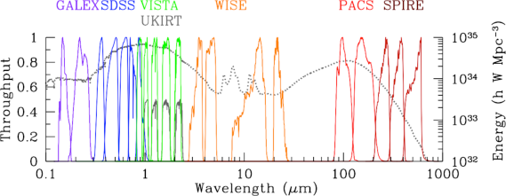
Figure 1: The 21 broad-band combined system throughput curves colour-coded by facility as indicated. Also shown (light grey line) is the recently measured(optical)/predicted(mid and far-IR) cosmic spectral energy distribution derived by Driver et al. (2012). This CSED can be thought of as an energy weighted “canonical” galaxy spectral energy distribution and highlights how the GAMA PDR filter set samples the key energy regime for nearby and low redshift galaxies. Note filters are scaled to a peak throughput of 1 except UKIRT which are scaled to 0.5 for clarity.

Table 1: The GAMA panchromatic imaging regions

GAMA region	SWarp RA centre	SWarp Dec centre	SWarp $\Delta$RA	SWarp $\Delta\delta$
G09	09:00:30	+00:15:00.0	19d15m24s	7d30m18s
G12	11:59:30	-00:15:00.0	19d15m24s	7d30m18s
G15	14:29:30	+00:15:00.0	19d15m24s	7d30m18s
G23	23:00:00	-32:30:00.0	14d00m00s	6d00m00s

Note: G02 is not included here but will be described in a dedicated release paper.

2 Panchromatic data genesis

Fig. 1 shows the wavelength grasp of the 21 broad-band filters. The response curves represent the combined system throughputs, normalised to a peak throughput of 1. Also shown as a line (in light grey) is the nearby energy output from the combined $z<0.1$ galaxy population derived from optical/near-IR analysis of the GAMA dataset (see Driver et al. 2012). This highlights how the various bands are sampling the stellar, polycyclic aromatic hydrocarbons (PAHs), warm (temperature $\sim 50$K) and cool (temperature $\sim 20$K) dust emissions of the low redshift galaxy population (the curve is shown for the energy output at $z=0$). In this section we start the process of constructing individual spectral energy distributions (SEDs) for every object within the GAMA main survey.

The first step is to place the diverse data onto a common astrometric grid. Table. 1 defines the extent of the GAMA PDR regions. We then use the Terapix SWarp package (see Bertin 2010) to build single image mosaics for each waveband and each region (see Hill et al. 2011). The SWarp package uses the tangent plane (TAN) World Coordinate System (WCS) to create a gnomic tangent-plane projection centred on the coordinates shown in Table 1. One might argue about the merit of constructing such large SWarped images ($\sim 110$ deg² each or up to 80GB for SDSS/VIKING data), however it was decided that this was preferable to managing the $\sim 1$ million non-aligned boundaries across the PDR. Taking each facility in turn we now describe the pre-processing necessary to construct our GAMA SWarps. Note that in addition to the native-resolution SWarps (see Table 2) we also construct a set of SWarps at a common 3.39^′′ resolution (i.e., 10 times the VISTA pixel scale) for later use in deriving coverage flags and background noise estimations.

2.1 GALEX MIS, GO and Archive data

The GALaxy Evolution eXplorer (GALEX, Martin et al. 2005) was a medium-class explorer mission operated by NASA and launched on April 28^th 2003. The satellite conducted a number of major surveys and observer motivated programs, most notably the all-sky imaging survey (AIS; typically 200s integrations per tile) and the medium imaging survey (MIS; typically 1500s per tile). The GALEX satellite is built around a 0.5-m telescope with a field-of-view of 1.13 deg², a pixel resolution of 1.5^′′, and a point-spread function FWHM of 4.2^′′ and 5.3^′′ in the FUV (153nm) and NUV (230nm) bands respectively (Morrissey et al. 2007). Imaging data sampled at 1.5 arcsec from V7 of the GALEX pipeline forms the basis for constructing the SWarped images. At the time of commencement of the GAMA survey the GAMA regions contained patchy coverage with GALEX. A dedicated programme led by one of us (RJT), was pursued providing further GALEX observations to MIS depth (1500s) and completed in April 2013 (using funds raised from the GAMA and Herschel-ATLAS Consortium to reactivate and extend the GALEX mission). The final collated data provides near-complete NUV and FUV coverage of the four primary GAMA regions. Due to the failure of the FUV channel mid-mission, the coverage at FUV in G23 is poor. However in G09, G12, and G15, coverage is at the 90% level in both bands (of which almost all is at MIS depth in the NUV, and 60 percent is at MIS depth in the FUV; see Section 2.6).

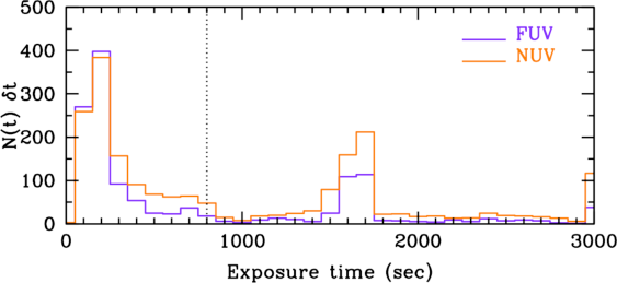
Figure 2: The distribution of exposure times contributing to the final FUV and NUV SWarps. The dotted vertical denotes the cutoff below which frames are not used in the final SWarps.

The analysis of the various GALEX datasets are described in detail in Andrae (2014) and summarised in Liske et al. (2015), and result in background subtracted intensity maps scaled to the common GALEX zero-points (Table 3). As the data originate from a variety of sources the exposure time is variable (see Fig. 2). To create our SWarps we take all available GALEX data frames with exposure times greater than 800s. Within the PDR only GALEX has such variable integration times.

In building the SWarps, a common circular mask (of radius 35^′) was used to trim the outer $\sim 5$ per cent of the image edges where the data quality degrades due to the vignetting of the telescope aperture (see Morrissey et al. 2007 and also Drinkwater et al. 2010 who adopted a similar radius for the WiggleZ survey). In total we have 150, 137, 175, and 22 GALEX pointings in FUV and 167, 175, 176 and 133 in the NUV for G09, G12, G15 and G23 respectively. These are combined to produce single image SWarps at the FUV and NUV native resolution for each region.

Note that a particular subtlety in building the FUV and NUV SWarps is the nature of the sky backgrounds. In the FUV the majority of pixels have zero flux (i.e., sky values of $<1$ photon) and hence the distribution of sky pixel-values is highly asymmetrical (i.e., Poissonian). Great care was taken by the GAMA GALEX team (MS, RJT, EA) to model and remove the backgrounds for each individual frame appropriately and provide to GAMA background subtracted FUV data (see Liske et al 2015, section 4.2 for further details). Hence when constructing the FUV SWarps the background subtraction option was switched off. Furthermore care should be taken in further background analysis of GALEX FUV data by only using mean statistics and not median statistics because of the highly asymmetrical background distribution, and ensuring sufficient counts within any aperture to derive a robust mean. The NUV data has a significant sky signal and is therefore processed with the SWarp background subtraction on using a $128\times 128$ pixel mesh (i.e., 198${}^{\prime\prime}\times$198^′′).

2.2 SDSS DR7

The Sloan Digital Sky Survey (York et al. 2000) provides uniform optical imaging of the G09, G12 and G15 regions in $ugriz$ bands at 0.4^′′ pixel resolution with a typical PSF FWHM of 1.4^′′ (see Hill et al. 2011, figure 3). As the GAMA spectroscopic survey was predicated on the SDSS imaging (Baldry et al. 2010) there is by design uniform $ugriz$ coverage of the three equatorial GAMA regions (G09, G12 and G15). In due course these regions, along with G23, are being surveyed by the KiDS team which will provide both deeper (2mag) and higher ($\times 2$) spatial resolution data (see de Jong et al. 2013).

Here we re-utilise the large mosaic GAMA SWarps built from the Sloan Digital Sky Survey Data Release 7 (Abazajian et al. 2009) by Hill et al. (2011, see update in Liske et al. 2015). In brief this involved the construction of both native seeing SWarps and SWarps built from data frames convolved to a uniform 2^′′ FWHM. The starting point is to download all contributing SDSS frames from the DR7 database, measure the PSF using PSFex (Bertin 2011), renormalise the data to a common zero-point, and produce both native seeing and convolved data frames (using fgauss within HEASoft to produce a common PSF FWHM of 2^′′). We then build SWarps at both the native and convolved resolutions from the distinct renormalised data frames. During the SWarping process (see Bertin 2010; Hill et al. 2011) the sky background is subtracted using a coarse $512\times 512$ pixel median filter to create a grid which in turn is median filtered $3\times 3$ before being fitted by a bi-cubic spline to represent the background structure. The use of a large initial median filter is to ensure minimal degradation of the photometry and shapes of extended systems.

G23 lies too far south to be observed by SDSS but along with G09, G12 and G15 are being observed to a uniform depth within the KiDS survey. The analysis of the KiDS data for GAMA and the preparation of the input catalogue for G23 will be presented in Moffett et al. (2015). At the present time optical SWarps for G23 do not exist.

2.3 VISTA VIKING

The Visible and Infrared Telescope for Astronomy (VISTA, Sutherland et al. 2015) is a 4.1m short focal length infrared optimised survey telescope located 1.5km from the VLT telescopes at Paranal Observatory. VISTA is owned and operated by ESO and commenced operations on 11^th December 2009. VISTA then entered a five year period of survey operation to conduct a number of ESO Public Surveys (Arnaboldi et al.  2007). One of these surveys, the VIsta Kilo-degree INfrared Galaxy Survey (VIKING), will cover 1500 deg² in two contiguous regions located in the north and south Galactic caps plus the G09 region. During the first two years of operations the VIKING survey prioritised the GAMA and Herschel-ATLAS survey regions. The VIKING survey footprint therefore covers all four primary GAMA regions (by design), in five pass bands ($ZYJHK_{s}$) at sub-arsecond resolution to projected $5\sigma$ point-source sensitivities of 23.1, 22.3, 22.1, 21.5, 21.2 AB mag (respectively).

The near-IR camera (VIRCAM, Dalton et al. 2006) consists of 16 Raytheon VIRGO HgCdTe arrays (detectors) sampling an instantaneous field-of-view of 0.6 deg² within the 1.65 deg diameter field. In routine operation a set of micro-dithered and stacked frames are formed, which are referred to as paw-prints. The on-camera dither sequence does not cover the gaps between the detectors and hence a sequence of six interleaved paw-prints is required to produce a contiguous coverage rectangular tile of 1.475 deg $\times$ 1.017 deg.

Paw-print data from the VISTA telescope is pipeline processed (Lewis, Irwin & Bunclark 2010) by the Cambridge Astronomy Survey Unit (CASU) to produce astrometrically and photometrically calibrated data. This process includes flat-fielding, bias subtraction, and linearity corrections. The paw-prints are then transmitted to the Wide Field Astronomy Unit (WFAU) at the Royal Observatory Edinburgh. The WFAU combines the paw-prints into the tiles which are then served to the community through both the ESO archive and the UK VISTA Science Archive (VSA). As the stacked tile data does not include sky-subtraction, sharp discontinuities can be introduced into the tiles. An additional concern is that the tiles may be constructed from paw-prints taken during significantly different seeing conditions. As we wish to both sky-subtract and homogenise the point-spread function to allow for aperture-matched photometry (see Hill et al. 2011), we requested access to all the VIKING paw-print data provided to the WFAU from CASU, which lay within the GAMA primary regions. This consisted of 9269 Rice compressed multi-extension fits files (v1.3 data from the CASU archive). These data were expanded out as individual detectors resulting in 148304 individual frames. Properties were extracted from the headers for each detector (airmass, extinction, exposure time, zero point, sky level, seeing) and the seeing measured directly using PSFex (Bertin 2011). The data for each individual detector were then rescaled to a common zero point (30) using Eqn. 1:

$${\rm I}_{\rm New}={\rm I}_{\rm Old}10^{(-0.4(Z-2.5\log_{10}(1/t)-(\tau(\sec\chi-1))+X_{\rm V.AB}-30))}$$ (1)

where $Z$ is the quoted zero-point, $t$ is the exposure time in seconds, $\tau$ is the extinction in the relevant band and $\sec\chi$ is the airmass. These values are obtained directly from the fits headers post-CASU processing. $X_{\rm V.AB}$ is the conversion from Vega to AB magnitudes (i.e., 0.521, 0.618, 0.937, 1.384 or 1.839 for Z,Y,J,H,K respectively) and were derived by CASU from the convolution of the complete system response functions convolved with the spectrum of Vega and a flat AB spectrum. The response functions in comparison to those for UKIRT are shown in Fig. 1.

These data were convolved with the Gaussian kernel required to produce a FWHM of $2^{\prime\prime}$ by assuming the PSF can be described as a Gaussian and that the convolution of two Gaussians produces a broader Gaussian, i.e., in line with our convolved SDSS data (see Hill et al. 2011). Fig. 3 shows the pre- and post- convolved FWHM as measured by PSFex. As can be seen the original seeing is predominantly sub-arcsecond as expected from the ESO Paranal (NTT peak) site and all the data lies well below our desired target PSF FWHM of 2^′′. Because the data is so much better than the target PSF FWHM value the assumption of a Gaussian profile should produce near-Gaussian final PSFs. Note that the $J$ band data is observed twice, increasing the abundance of independent measurements. The post-processed data is centred close to the target PSF FWHM of $2^{\prime\prime}$ with some indication of slight systematics between the bands at the $5$ per cent level. Note this is not a major concern as we use apertures with minimum major or minor diameters of $5^{\prime\prime}$ when measuring our $u-K_{s}$ aperture-matched photometry (see Section 3.1).

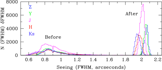
Figure 3: Pre and post convolution seeing measurements of the 148304 VISTA VIKING frames using PSFex.

From our initial SWarps we noted that a portion of data is clearly of very low quality (see Fig. 4). We therefore elected to inspect a subset of the data by selecting three categories: outliers defined as those with seeing better than 0.5^′′ or worse than 1.5^′′, a zero-point multiplier of greater than 40, a sky value of less than 100 ADU counts or a CASU tilecode not equal to 0, 56, or -1, i.e., 9535 frames in total; control defined as a random set of 1000 frames not included in the above selection; and sparse defined as every detector 8 frame not already included in one of the earlier samples, i.e., 6945 frames. These 16590 frames were inspected by two of us (SPD, AHW) using the mogrify routine within the imagemagick package to generate greyscale images where the lowest 2 per cent of data were set black, the highest 10 per cent white, and with histogram equalisation in-between. This scaling amplifies background gradients rendering even the best quality data in the poorest light (see Fig. 4). We then rejected or accepted the frames via visual inspection and attempted to identify a measurable quantity which best separated out the rejected frames, see Fig. 5. This resulted in the adoption of a simple cut on the zero-point multiplier factor, whereby all frames which require a rescaling of $\times 30$ or more are rejected in addition to those already identified from the visual inspections. In total 3262 of our 148304 frames were rejected (i.e., 2.2 per cent of the data). Examples of accepted and rejected frames are shown in Fig. 4 and common causes are bright sky, detector failures and telescope pointing errors.

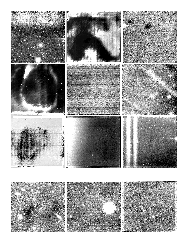
Figure 4: Examples of poor quality (top three rows) and acceptable quality (bottom row) VIKING frames. Approximately 12 per cent of the VIKING data were visually inspected based on outlying values in airmass, sky background, zero-point, and seeing.

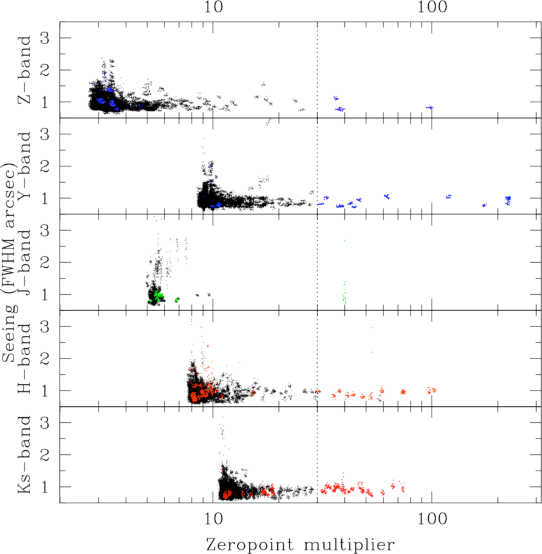
Figure 5: Seeing versus zero-point multiplier for each band (as indicated). A cut of 30 appears to isolate the majority of low quality frames (indicated by the coloured points).

The remaining frames were then SWarped (Bertin et al. 2010) to the GAMA PDR regions specified in Table 1 with a pixel size of 0.339^′′ using the TAN WCS projection. During the SWarping process the background for each contributing detector was removed using a $128\times 128$ pixel median filter which in turn was median filtered by a $3\times 3$ grid before being fitted with a bi-cubic spline. The choice of background filter size is critical; too high and the structure of the tiling becomes apparent in the SWarp (see Fig. 6), too low and galaxy photometry can be affected (see Fig. 7). To optimise the background filter size we produced frames with a range of background filter sizes and performed structural analysis of the brightest 100 galaxies using SIGMA (Kelvin et al. 2012). Fig. 8 shows the magnitude offsets and Fig. 9 shows how the measured major-axis half-light radii vary with background mesh size. We tested pixel grids of $512\times 512$, $256\times 256$, $128\times 128$ and $64\times 64$ and only the smallest filter size had any noticeable impact on the measured properties and hence the second smallest filter size was adopted. Note that this finer filtering (compared to SDSS) is absolutely necessary because of (a) the mode of observation (pointed v drift-scan) and (b) the higher-degree of sky spatial variations in the near-IR wavebands.

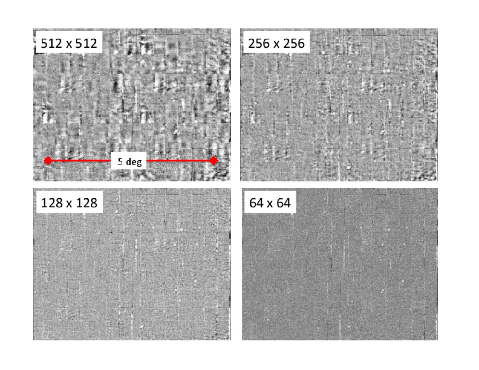
Figure 6: Examples of sections of VIKING data with various background subtractions as indicated.

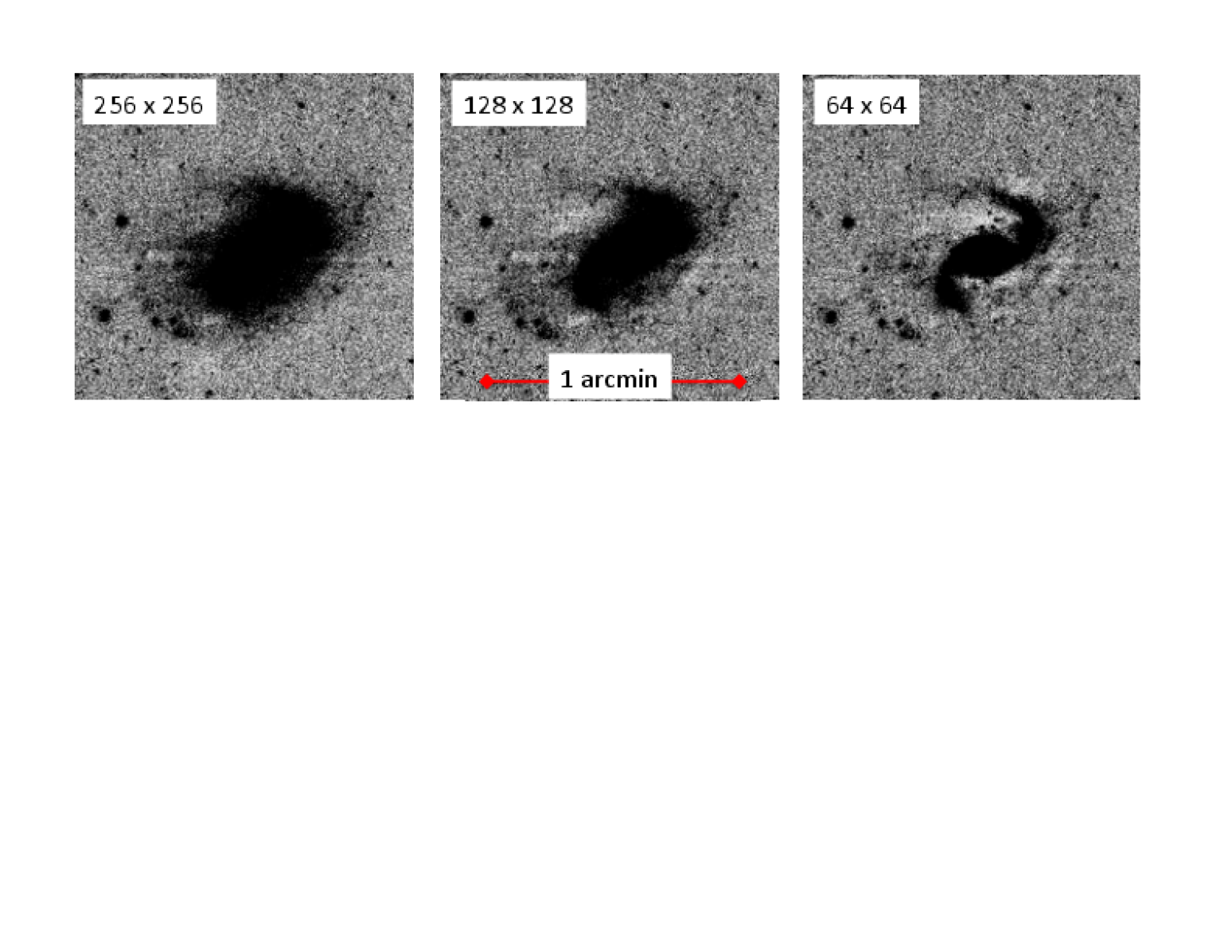
Figure 7: An illustration of the impact of over-smoothing the background on extended objects. The galaxy shown is the largest system in the GAMA region, NGC0895 (located in G02). In the rightmost panel a significant portion of the galaxy has been removed due to the $64\times 64$ pixel sky-subtraction process.

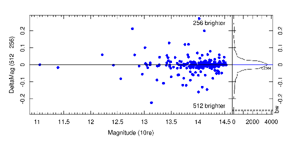
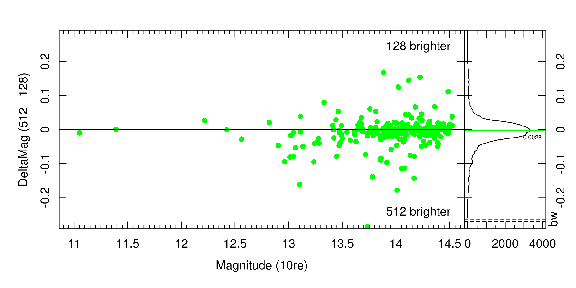
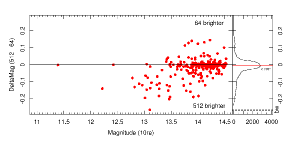
Figure 8: A comparison of flux measurements of the brightest 100 galaxies with varying background subtraction meshes. In each case the flux is compared against that derived from the $512\times 512$ pixel background mesh. In general it is only galaxies brighter than 14^th magnitude with the $64\times 64$ background mesh whose photometry is compromised.

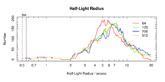
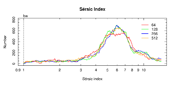
Figure 9: The major-axis half-light radius (upper panel) and the Sérsic index distributions (lower panel) for the brightest 100 galaxies for various background mesh sizes as indicated.

2.4 WISE

The Wide-Field Infrared Survey Explorer (WISE; Wright et al. 2010) is a medium-class explorer mission operated by NASA and was launched on 14^th December 2009. Following approximately 1 month of checks WISE completed a shallow survey of the entire sky in 4 infrared bands (3.4, 4.6, 12 and 22$\mu m$) over a ten month period. WISE is built around a 40-cm telescope with a $47^{\prime}\times 47^{\prime}$ field-of-view, and scans the sky with an effective exposure time of 11s per frame. Each region of sky is typically scanned from tens to hundreds of times (with fields further from the ecliptic being observed more frequently). This allows the construction of deep stacked frames reaching a minimum $5\sigma$ point source sensitivity of 0.08, 0.11, 0.8 and 4 mJy in the W1(3.4$\mu m$), W2(4.6$\mu m$), W3(12$\mu m$) and W4(22$\mu m$) bands (see Wright et al. 2010). The base “Atlas” data consists of direct stacks and associated source catalogues which are publicly available via the WISE and AllWISE data release hosted by the Infrared Science Archive (IRSA). These public data have point-spread function FWHM resolutions of $\sim 8.4^{\prime\prime},9.2^{\prime\prime},11.4^{\prime\prime}$ and $18.6^{\prime\prime}$ in W1, W2, W3 and W4 respectively and a 1.375^′′/pixel scale. However, because of the stability of the point-spread function of the WISE system, higher resolution can be attained using deconvolution techniques, in particular “drizzled” co-addition and the Maximum Correlation Method of Masci & Fowler (2009; see Jarrett et al. 2012). Here we use data which has been re-stacked via the drizzle method as the MCM or HiRes method is computationally expensive and only suited for very large nearby galaxies (see Jarrett et al. 2012, 2013). In brief this involves:

(1) gain-matching and rescaling the data ensuring a common photometric zero-point calibration,

(2) background level offset-matching,

(3) flagging and outlier rejection,

(4) co-addition using overlap area weighted interpolation and drizzle.

Here drizzle refers to the Variable Pixel Linear Reconstruction technique of co-addition using a Point Response Function kernel to construct the mosaics. Full details are provided in the WISE ICORE documentation (Masci 2013). The drizzled data results in final point-source FWHM of $5.9^{\prime\prime},6.5^{\prime\prime},7.0^{\prime\prime}$, and $12.4^{\prime\prime}$ (respectively), see Cluver et al. (2014) and Jarrett et al. (2012) for further details. Fig. 10 shows a comparison for one of our GAMA galaxies between the “Atlas” and drizzled image in each of the four bands. The “drizzled” frames are provided to the GAMA team stacked, calibrated to a common zero point, and background subtracted in sections of $1.56^{\circ}\times 1.56^{\circ}$. These frames are then SWarped into a single large mosaic at the native pixel resolution of $1^{\prime\prime}$ using the same field centre, and projection system as for the previous datasets. In re-gridding the data we also include the SWARP background subtraction using a $256\times 256$ pixel filter.

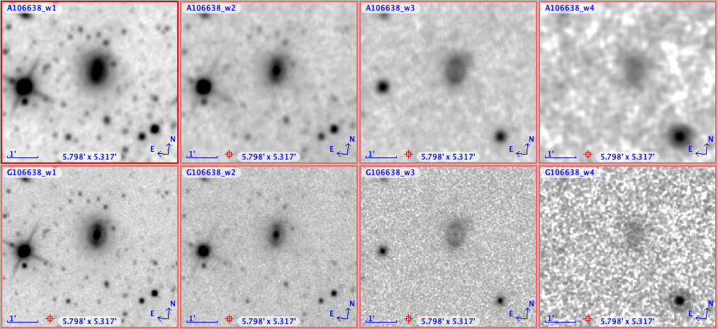
Figure 10: A visual comparison of WISE Atlas images (upper rows) and WISE drizzled images (lower rows) for bands W1, W2, W3, W4 (left-to-right). The panels are displayed over comparable ranges and the improvement in spatial resolution via the drizzling technique is self-evident. For details of the drizzling technique see Jarrett et al. (2012).

2.5 Herschel-ATLAS

The Herschel Space Observatory (Pilbratt et al. 2010) is operated by the European Space Agency and was launched on May 14^th 2009 and conducted a number of major survey campaigns during its 3.5 years of operation. The largest extragalactic survey, in terms of areal coverage, is The Herschel Astrophysical Terahertz Large Area Survey (Herschel-ATLAS; Eales et al. 2010). Herschel-ATLAS images were obtained using Herschel’s fast-scan parallel mode and covered $\sim$600 deg² of sky in five distinct sky regions which included the four principal GAMA fields. The co-ordinated observations used both the PACS (Poglitsch et al. 2010) and SPIRE (Griffin et al. 2010) instruments to obtain scans at 100$\mu m$, 160$\mu m$, 250$\mu m$, 350$\mu m$, 500$\mu m$, i.e., sampling the warm and cold dust components of galaxies from z=0 to z=4. The final maps were the combination of two orthogonal cross-scans giving rise to PSFs with Gaussianised FWHM of 9.6^′′ and 12.5^′′ in 100 and 160$\mu m$ and 18^′′, 25^′′ and 35^′′ in the 250, 350 and 500 $\mu m$ bands respectively (see Valiante et al. 2015 for full details of the PSF characterisation). The data were processed, calibrated, nebularized to remove large scale fluctuations due to cirrus and large scale clustering of high-z sources, (see Valiante et al.2015. and Maddox et al. 2015), and finally mosaiced by the Herschel-ATLAS data reduction team who provided the final maps and 5$\sigma$ source detection catalogues. The reduction process for the two instruments are described in detail in Ibar et al. (2010), and Pascale et al. (2011), to be superseded shortly by Valiante et al. (2015), and the method for source detection is described in detail in Rigby et al. (2011) also updated in Valiante et al. (2015). The absolute zero point calibration is accurate to $\pm 10$ per cent for PACS and $\pm 7$ per cent for SPIRE which provides a potential systematic pedestal in addition to the random sky and object photon noise errors estimated later. Note that as the Herschel-ATLAS data have not yet been publicly released they remain subject to change. Every attempt will be made to ensure the online GAMA PDR provides notifications of any changes or updates.

To date the Herschel-ATLAS data have been used to study the dust and star-formation properties of both near and distant galaxies based on far-IR/optical matched samples (see for example Dunne et al. 2011; Smith et al. 2011, 2012; Bourne et al. 2012 Rowlands et al. 2012). To pre-prepare the data for GAMA we re-SWarp the mosaics provided onto a uniform grid using the field centres from Table 1 using the TAN WCS projection, and preserving the original pixel size as specified in the file headers and shown on Table 2.

Table 2: Key meta-data information of the contributing datasets.

Facility	Dataset	Instrument	Filter	Pivot	Pixel	Point-source	Frames	$m_{\rm AB}-m_{\rm Vega}$
	or survey	or technique	name	Wavelength	Resolution	FWHM	Supplied	(mag)
GALEX	MIS+GO	-	FUV	1535Å	1.5′′	4.1′′	279	2.16
GALEX	MIS+GO	-	NUV	2301Å	1.5′′	5.2′′	297	1.67
SDSS	DR7	-	$u$	3557Å	0.339′′	1.4′′	26758	0.98
SDSS	DR7	-	$g$	4702Å	0.339′′	1.4′′	26758	-0.10
SDSS	DR7	-	$r$	6175Å	0.339′′	1.4′′	26758	0.15
SDSS	DR7	-	$i$	7491Å	0.339′′	1.4′′	26758	0.38
SDSS	DR7	-	$z$	8946Å	0.339′′	1.4′′	26758	0.54
VISTA	VIKING	VIRCAM	$Z$	8800Å	0.339′′	0.85′′	15360	0.521
VISTA	VIKING	VIRCAM	$Y$	10213Å	0.339′′	0.85′′	15797	0.618
VISTA	VIKING	VIRCAM	$J$	12525Å	0.339′′	0.85′′	34076	0.937
VISTA	VIKING	VIRCAM	$H$	16433Å	0.339′′	0.85′′	15551	1.384
VISTA	VIKING	VIRCAM	$Ks$	21503Å	0.339′′	0.85′′	16340	1.839
WISE	AllSky	drizzled	$W1$	3.37$\mu m$	1′′	5.9′′	40	2.683
WISE	AllSky	drizzled	$W2$	4.62$\mu m$	1′′	6.5′′	40	3.319
WISE	AllSky	drizzled	$W3$	12.1$\mu m$	1′′	7.0′′	40	5.242
WISE	AllSky	drizzled	$W4$	22.8$\mu m$	1′′	12.4′′	40	7.871
Herschel	ATLAS	PACS	100$\mu m$	101$\mu m$	3′′	9.6′′	4 (& 1 for G23)	N/A
Herschel	ATLAS	PACS	160$\mu m$	161$\mu m$	4′′	12.5′′	4 (& 1 for G23)	N/A
Herschel	ATLAS	SPIRE	250$\mu m$	249$\mu m$	6′′	18′′	4 (& 1 for G23)	N/A
Herschel	ATLAS	SPIRE	350$\mu m$	357$\mu m$	8′′	25′′	4 (& 1 for G23)	N/A
Herschel	ATLAS	SPIRE	500$\mu m$	504$\mu m$	12′′	36′′	4 (& 1 for G23)	N/A

Table 3: Surface brightness limits of our GAMA SWarp set (FUV to mid-IR).

SWarp	Zero-Point	SWarp mean	$1\sigma_{\rm Sky}$	5$\sigma$ limit		Coverage
Facility/Filter/Field	(AB mag for 1ADU)	(/′′)	(mag arcsec-2)†	(mag)‡	(Jy)⋄	(%)
GALEX FUV G09	$18.82$	$0.000148$	$28.41$	$25.23$	$2.94E-07$	88
GALEX FUV G12	$18.82$	$5.04E-05$	$29.58$	$26.40$	$1E-07$	92
GALEX FUV G15	$18.82$	$0.00013$	$28.54$	$25.37$	$2.59E-07$	95
GALEX FUV G23	$18.82$	$0.000266$	$27.77$	$24.59$	$5.31E-07$	75
GALEX NUV G09	$20.08$	$0.00125$	$27.35$	$23.92$	$9.84E-07$	94
GALEX NUV G12	$20.08$	$0.00116$	$27.43$	$23.99$	$9.17E-07$	97
GALEX NUV G15	$20.08$	$0.00161$	$27.07$	$23.64$	$1.27E-06$	95
GALEX NUV G23	$20.08$	$0.00109$	$27.50$	$24.07$	$8.58E-07$	99
SDSS $u$ G09	$30.00$	$142$	$24.61$	$22.24$	$4.61E-06$	100
SDSS $u$ G12	$30.00$	$163$	$24.47$	$22.09$	$5.28E-06$	100
SDSS $u$ G15	$30.00$	$156$	$24.51$	$22.14$	$5.06E-06$	100
SDSS $g$ G09	$30.00$	$54.3$	$25.66$	$23.29$	$1.76E-06$	100
SDSS $g$ G12	$30.00$	$65.3$	$25.46$	$23.09$	$2.12E-06$	100
SDSS $g$ G15	$30.00$	$62.6$	$25.50$	$23.13$	$2.03E-06$	100
SDSS $r$ G09	$30.00$	$76.7$	$25.28$	$22.91$	$2.49E-06$	100
SDSS $r$ G12	$30.00$	$95.4$	$25.05$	$22.67$	$3.09E-06$	100
SDSS $r$ G15	$30.00$	$90.5$	$25.10$	$22.73$	$2.93E-06$	100
SDSS $i$ G09	$30.00$	$116$	$24.84$	$22.47$	$3.75E-06$	100
SDSS $i$ G12	$30.00$	$140$	$24.62$	$22.25$	$4.56E-06$	100
SDSS $i$ G15	$30.00$	$129$	$24.72$	$22.35$	$4.19E-06$	100
SDSS $z$ G09	$30.00$	$506$	$23.23$	$20.86$	$1.65E-05$	100
SDSS $z$ G12	$30.00$	$579$	$23.09$	$20.71$	$1.88E-05$	100
SDSS $z$ G15	$30.00$	$556$	$23.13$	$20.76$	$1.81E-05$	100
VIKING Z G09	$30.00$	$59.8$	$25.55$	$23.18$	$1.94E-06$	100
VIKING Z G12	$30.00$	$60.6$	$25.54$	$23.17$	$1.97E-06$	100
VIKING Z G15	$30.00$	$62$	$25.51$	$23.14$	$2.01E-06$	99
VIKING Z G23	$30.00$	$67.9$	$25.41$	$23.04$	$2.2E-06$	100
VIKING Y G09	$30.00$	$123$	$24.77$	$22.40$	$3.98E-06$	100
VIKING Y G12	$30.00$	$110$	$24.89$	$22.52$	$3.56E-06$	100
VIKING Y G15	$30.00$	$111$	$24.88$	$22.51$	$3.61E-06$	100
VIKING Y G23	$30.00$	$129$	$24.71$	$22.34$	$4.2E-06$	100
VIKING J G09	$30.00$	$167$	$24.44$	$22.06$	$5.43E-06$	100
VIKING J G12	$30.00$	$161$	$24.48$	$22.10$	$5.23E-06$	100
VIKING J G15	$30.00$	$146$	$24.58$	$22.21$	$4.74E-06$	100
VIKING J G23	$30.00$	$155$	$24.52$	$22.14$	$5.04E-06$	100
VIKING H G09	$30.00$	$329$	$23.70$	$21.33$	$1.07E-05$	98
VIKING H G12	$30.00$	$302$	$23.79$	$21.42$	$9.82E-06$	99
VIKING H G15	$30.00$	$313$	$23.75$	$21.38$	$1.02E-05$	97
VIKING H G23	$30.00$	$325$	$23.71$	$21.34$	$1.06E-05$	100
VIKING K G09	$30.00$	$332$	$23.69$	$21.32$	$1.08E-05$	100
VIKING K G12	$30.00$	$337$	$23.67$	$21.30$	$1.09E-05$	100
VIKING K G15	$30.00$	$303$	$23.79$	$21.42$	$9.83E-06$	100
VIKING K G23	$30.00$	$285$	$23.86$	$21.48$	$9.25E-06$	100
WISE W1 G09	$23.18$	$0.262$	$24.64$	$21.09$	$1.33E-05$	100
WISE W1 G12	$23.18$	$0.281$	$24.56$	$21.01$	$1.43E-05$	100
WISE W1 G15	$23.14$	$0.21$	$24.84$	$21.29$	$1.11E-05$	100
WISE W1 G23	$23.14$	$0.187$	$24.96$	$21.41$	$9.9E-06$	100
WISE W2 G09	$22.82$	$0.327$	$24.04$	$20.38$	$2.55E-05$	100
WISE W2 G12	$22.82$	$0.367$	$23.91$	$20.26$	$2.87E-05$	100
WISE W2 G15	$22.82$	$0.264$	$24.27$	$20.61$	$2.06E-05$	100
WISE W2 G23	$22.82$	$0.229$	$24.42$	$20.77$	$1.79E-05$	100

^† $\mu_{1\sigma}=ZP-2.5\log_{10}({\rm\sigma_{\rm ADU}})$.

^‡ $5\sigma~{}{\rm limit}=ZP-2.5\log_{10}(5\sqrt{\pi HWHM^{2}}\sigma_{\rm ADU})$ where HWHM is Half Width Half-Maximum of the seeing-disc (i.e., 0.5 FWHM).

^⋄ $F_{\nu}(Jy)=3631\times 10^{-0.4{\rm mag}_{5\sigma{\rm limit}}}$

Table 4: Surface brightness limits of our GAMA SWarp set (mid-IR to far-IR.

SWarp	Zero-Point	SWarp mean	$1\sigma_{\rm Sky}$	5$\sigma$ limit		Coverage
Facility/Filter/Field	(AB mag for 1ADU)	(/′′)	(mag arcsec-2)†	(mag)‡	(Jy)⋄	(%)
WISE W3 G09	$23.24$	$2.33$	$22.32$	$18.59$	$0.000133$	100
WISE W3 G12	$23.24$	$2.68$	$22.17$	$18.44$	$0.000153$	100
WISE W3 G15	$23.24$	$1.77$	$22.62$	$18.89$	$0.000101$	100
WISE W3 G23	$23.24$	$2.18$	$22.39$	$18.66$	$0.000125$	100
WISE W4 G09	$19.60$	$0.278$	$20.99$	$16.64$	$0.000802$	100
WISE W4 G12	$19.60$	$0.305$	$20.89$	$16.54$	$0.000879$	100
WISE W4 G15	$19.60$	$0.208$	$21.31$	$16.96$	$0.000599$	100
WISE W4 G23	$19.60$	$0.265$	$21.05$	$16.69$	$0.000762$	100
PACS 100 G09	$8.90$	$0.000562$	$-$	$12.96$	$0.0894$	100
PACS 100 G12	$8.90$	$0.000545$	$-$	$12.99$	$0.0879$	100
PACS 100 G15	$8.90$	$0.000547$	$-$	$12.99$	$0.0863$	100
PACS 100 G23	$8.90$	$0.000476$	$-$	$13.14$	$0.0795$	100
PACS 160 G09	$8.90$	$0.000278$	$-$	$13.44$	$0.103$	100
PACS 160 G12	$8.90$	$0.000273$	$-$	$13.46$	$0.101$	100
PACS 160 G15	$8.90$	$0.000271$	$-$	$13.47$	$0.101$	100
PACS 160 G23	$8.90$	$0.000227$	$-$	$13.66$	$0.0903$	100
SPIRE♭ 250 G09	$11.68$	$0.000759$	$-$	$12.56$	$0.0343$	80
SPIRE♭ 250 G12	$11.68$	$0.00073$	$-$	$12.60$	$0.0330$	81
SPIRE♭ 250 G15	$11.68$	$0.00073$	$-$	$12.59$	$0.0333$	84
SPIRE♭ 250 G23	$11.68$	$0.000885$	$-$	$12.52$	$0.0357$	100
SPIRE♭ 350 G09	$11.67$	$0.000447$	$-$	$12.36$	$0.0412$	80
SPIRE♭ 350 G12	$11.67$	$0.000424$	$-$	$12.41$	$0.0394$	81
SPIRE♭ 350 G15	$11.67$	$0.000423$	$-$	$12.41$	$0.0393$	84
SPIRE♭ 350 G23	$11.67$	$0.000518$	$-$	$12.51$	$0.0357$	100
SPIRE♭ 500 G09	$11.62$	$0.000228$	$-$	$12.16$	$0.0495$	80
SPIRE♭ 500 G12	$11.62$	$0.000217$	$-$	$12.23$	$0.0467$	81
SPIRE♭ 500 G15	$11.62$	$0.000221$	$-$	$12.21$	$0.0476$	84
SPIRE♭ 500 G23	$11.62$	$0.000257$	$-$	$12.17$	$0.0490$	100

^† $\mu_{1\sigma}=ZP-2.5\log_{10}({\rm\sigma_{\rm ADU}})$.

^‡ $5\sigma~{}{\rm limit}=ZP-2.5\log_{10}(5\sqrt{\pi HWHM^{2}}\sigma_{\rm ADU})$ where HWHM is Half Width Half-Maximum of the seeing-disc (i.e., 0.5 FWHM).

^⋄ $F_{\nu}(Jy)=3631\times 10^{-0.4{\rm mag}_{5\sigma{\rm limit}}}$

^♭ SPIRE maps are in units of Jansky per Beam and to generate these zero-points we have added a factor $2.5\log_{10}(B/N^{2})$ where B is the beam size given as 466, 821, and 1770 sq arcsec in 250, 350 and 500$\mu$m respectively and N is the pixel size given in Table 2.

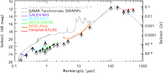
Figure 11: The sensitivity reached in each band as derived from the GAMA SWarps (black lines) and compared to the listed values (coloured lines). Also shown in grey is a typical SED for a dusty galaxy with $r_{\rm AB}=19.8$ mag.

2.6 Cosmetic and noise characteristics of the GAMA SWarp set

To assess the quality of GAMA SWarps we derive the background noise distributions (i.e., sky-subtracted), within selected regions for each of our LOW-RES (i.e., 3.39^′′) SWarps, which are displayed from $-2\sigma$ to $+2\sigma$ in Figs. A27 to A30 for G09, G12, G15 and G23 respectively. The black rectangle represents the GAMA region and the dotted blue rectangle the selected region from which the noise characteristics are derived (the mode and 3$\sigma$-clipped standard deviation). These images show no obvious major sky gradients across the sky regions, however, they do show interesting substructure which highlights correlations in the underlying noise properties. In most cases the correlations highlight the genesis, i.e., the SDSS stripes, GALEX pointings, and VIKING paw-prints. In these cases the noise properties for each particular frame/scan is dictated by the conditions during observations (SDSS and VISTA) or the variability of the various integration times (GALEX). While uniform backgrounds are highly desirable, these are never achieved in practice. Some SDSS scans will be slightly less noisy than others and some paw-prints will have significantly amplified noise characteristics. Interestingly the WISE and Herschel-ATLAS data show the least structure which mainly reflects the benefits of using fixed integration times as well as operating outside the confines of a time-varying atmosphere. However, some impact of observing close to the moon is apparent in the WISE G12 SWarps. Also noticeable in the Herschel-ATLAS data is the reduced noise in the overlap regions as expected.

The noise distributions derived from the GAMA SWarps are shown in Table 3, for GALEX, SDSS, VISTA and WISE data these statistics are derived from fitting a Gaussian distribution to the histogram of data values below the mode. They therefore do not include any confusion estimate and assume the noise is uncorrelated. In all cases the distributions are very well described by a normal distribution implying that the systematic frame-pistoning (i.e., ZP offsets) in the data (arising from the independent calibration of the distinct pointings), is operating at a relatively low level and within the range of the pixel-to-pixel variations. Using the $3\sigma$-clipped standard deviations we derive (analytically) the 1$\sigma$ surface brightness limits and the 5$\sigma$ point-source detection limits for each of the SWarp images (see Table. 3). For the PACS and SPIRE data, where correlated noise is believed to be an issue, we derive the 5$\sigma$ detection limits directly by placing apertures equivalent to the Beam size at random locations across the SWarps and measuring the standard deviation of the resulting aperture fluxes (again fitting to the distribution below the mode). In Fig. 11 the GAMA SWarp detection limits are compared to the values listed online for each facility (as indicated by the colour lines). For GALEX MIS, SDSS DR7, and VIKING, the depths probed agree extremely well. Note that our derived WISE W1 band limit appears significantly deeper than that quoted by the WISE collaboration this is because our values ignore confusion (i.e., fits to the negative noise distribution) whereas the WISE quoted value incorporates this aspect. For Herschel-ATLAS SPIRE we note that the agreement with the SPIRE values reported in Valiante et al. (2015) is extremely good.

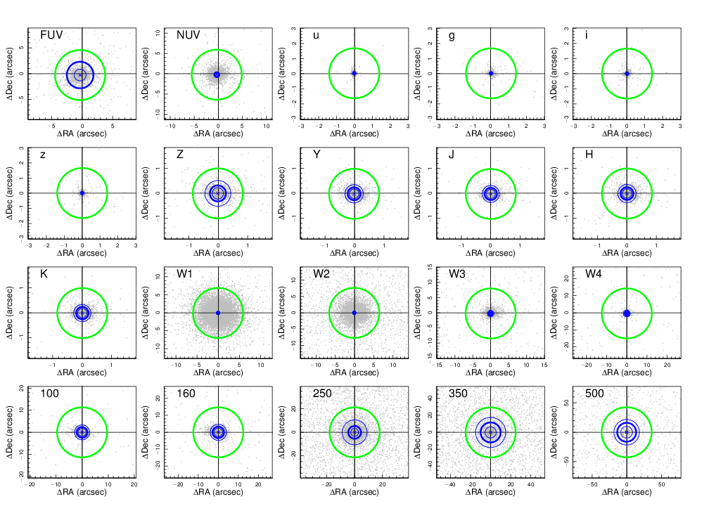
Figure 12: Confirmation of the astrometric accuracy. Each diagram shows the positional offsets of that particular band against the $r$ band GAMA Input or Tiling catalogues (grey data points). The centroid of the population is shown with a blue cross and the (native) PSF FWHM is shown as a green circle. The circles enclosing 50, 66 and 80 per cent of the population is shown by a thin, thick and thin blue line respectively. In all cases the relative astrometry is robust to $<0.1$PSF FWHM, and the 66 per cent spread enclosed with $0.5\times$ the PSF FWHM.

2.7 Astrometric verification

To check the astrometric alignment of the SWarps we run SExtractor over either the entire SWarp set (GALEX, WISE, and Herschel) or a 4sq deg section from G12 (SDSS and VIKING, to keep CPU requirement manageable). We use relatively high signal-to-noise cuts of 100 (GALEX, where the data is not uniform), 10 (WISE and Herschel), or 3 (SDSS and VIKING). We then match to either the GAMA InputCat with $r<17.0$ mag (GALEX, SDSS, VIKING and WISE) or the GAMA TilingCatv45 with $r<17.0$ mag and $(u-g)<1.5$ (Herschel-ATLAS) to isolate star-forming galaxies. Fig. 12 shows the resulting $\Delta$ RA and $\Delta$ Dec diagrams for each band compared to the canonical $r$-band data (grey data points). On Fig. 12 the blue cross (mostly not visible) defines the centroid and the thick green circle indicates the PSF FWHM for that band. The thick blue band defines the region which encloses 66 percent of the population (after accounting for the density of random mis-matches), and the thin blue circles enclose either 50 percent or 80 percent of valid matches. Fig. 12 highlights that in all cases the centroid of the RA and Dec offset is extremely close to zero (below 0.3^′′ in all bands with the FUV and NUV showing the largest offsets, and below 0.02^′′ in the optical and near-IR), and that the 66 percent sprawl lies within $0.5\times$ the PSF FWHM in all bands. We therefore consider the astrometry to be as one would expect given the respective FWHM seeing values.

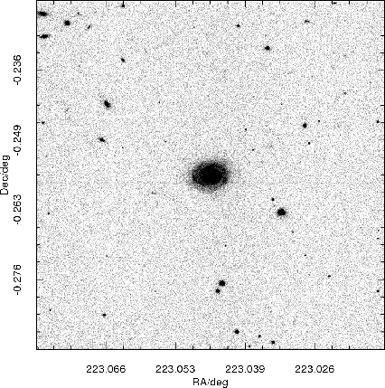
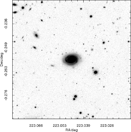
Figure 13: A comparison of the quality of the SDSS $z$ band data (left) against the VISTA VIKING $Z$ band (right).

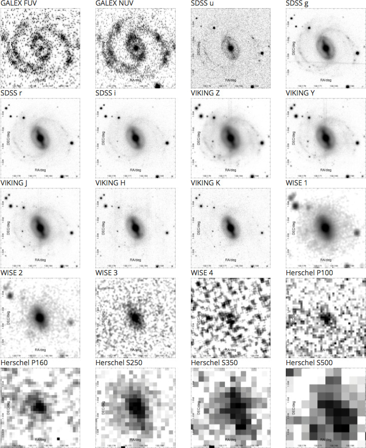
Figure 14: 20 band panchromatic imaging for a $1^{\prime}\times 1^{\prime}$ region centred on GAMA galaxy G371633. Filters increase in wavelength proceeding from left to right and top to bottom, note the SDSS $z$ filter is omitted, i.e., FUV, NUV, u, g, r, i, Z, Y, J, H, K, W1, W2, W3, W4, 100, 160, 250, 350, 500. Produced using the GAMA $\Psi$: http://gama-psi.icrar.org/

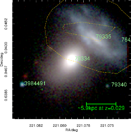
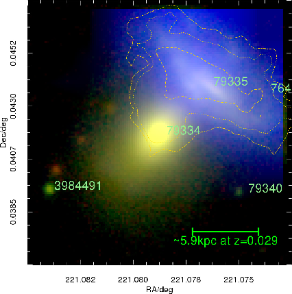
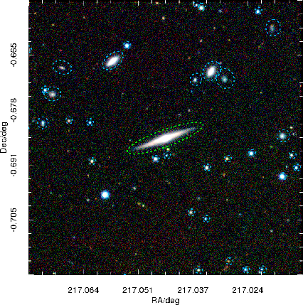
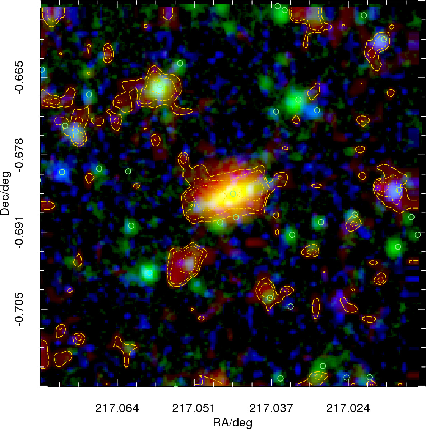
Figure 15: Upper left: A colour composite image of G79334 produced by combining the SDSS $g$ & $r$ with the VIKING H band images. Overlaid are the contours from SPIRE-250 band. GAMA IDs are marked. Upper right: A colour composite of G79334 from GALEX NUV, VIKING $Z$ & $K_{s}$ and with contours overlaid from WISE. Lower left: A $2^{\prime}\times 2^{\prime}$ colour composite centred on G48432 made from data extracted from the GAMA SDSS $r$ & $i$ SWarp combined with the VIKING $H$ SWarp and with the apertures used for the aperture-matched photometry overlaid. (lower right) A composite colour image of G48432 made from GALEX FUV (blue channel), WISE W1 (green channel) and SPIRE 250$\mu m$ (red channel and contours). All images produced using the online GAMA $\Psi$ tool: http://gama-psi.icrar.org/

2.8 Visual inspection of the combined data and data access

Our full dataset is diverse and the volume large. In order to inspect the data we have developed a publicly available online tool which provides both download links to the individual SWarps, as well as an option to extract image regions from the dataset. Users can also build RGB colour images using any of the 21 bands as well as overlay contours and basic catalogue information (e.g., GAMA IDs, photometry apertures, and object locations). The GAMA Panchromatic SWarp Imager ($\Psi$) is therefore extremely versatile and useful for exploring the data volume:

http://gama-psi.icrar.org/

Fig. 13,  14 & 15 show examples of various extractions using the tool with Fig. 13 showing the significant increase in depth from the SDSS $z$ band data to the VISTA VIKING $Z$ band. Fig. 14 shows a single GAMA galaxy in 20 of the 21 bands (note that the SDSS $z$ band is not shown here), and Fig. 15 shows various colour combinations with contours, IDs and apertures overlaid as indicated. Note that searches can be made based on GAMA ID or RA and Dec and is therefore of use to high-z teams with objects in the GAMA regions (e.g., Herschel-ATLAS team).

Using GAMA $\Psi$ via the link above, one can also access the individual SWarps files including the native, convolved and weight-maps and the XML files which contain, the pixel data, a description of the weights, and a listing of the constituent files making up the SWarp respectively. The weight-maps are particularly useful and can be used to determine both the coverage and provide a mask. Zero values in the weight SWarp imply no data while non-zero values imply coverage. These weight-maps have been used to generate the coverage statistics shown in col. 7 of Table. 3. The SWarps, weight-maps, and XML files can all be downloaded from:

http://gama-psi.icrar.org/panchromaticDR.php

However, note that files sizes vary from 100KB (for XML files) to up to 80GB (for SWarps and weight-maps).

3 Panchromatic photometry for G09, G12 and G15 only

Vital to successful analysis of panchromatic data are robust flux measurements, robust errors, and a common deblending solution. This is particularly difficult when the flux sensitivities and spatial resolutions vary significantly, as is the case with the GAMA PDR (see Figs 11, 14 & 15, i.e., 35^′′ to 0.7^′′ spatial resolution). In an ideal situation one would define an aperture in a single band and then place the same aperture at the same astrometric location in data with identical spatial sampling. This is the strategy we pursued in Hill et al. (2011, see also Driver et al. 2011) to derive $u-K_{s}$ aperture-matched photometry (using the seeing-convolved SWarps convolved to a 2^′′ FWHM). While we can still implement this strategy in the $u$ to $K_{s}$ range (see Section 4.2 below) we cannot easily extend it outside this wavelength range because of the severe resolution mismatch (see Table 2). Software (LAMBDAR) is being developed to specifically address this issues and will be described in a companion paper (Wright et al. 2015). In the meantime, we assemble a benchmark panchromatic catalogue from a combination of aperture-matched photometry, table matching, and optically-motivated (forced) photometry. It is worth noting that the GAMA PDR assembled here while heterogeneous across facilities is essentially optimised for each facility, and therefore optimal for studies not requiring broad panchromatic coverage.

In the FUV and NUV, we use the GAMA GALEX catalogue described in Liske et al. (2015) and which uses a variety of photometry measures including curve-of-growth and the GALEX pipeline fluxes. In the optical and near-IR we apply the aperture-matched method mentioned above and described in detail in the next sections. In the mid-IR we use the WISE catalogues described in Cluver et al. (2014). Longwards of the WISE bands we adopt a strategy developed by the Herschel-ATLAS team (Bourne et al. 2012, see Appendix A) to produce optically-motivated aperture measurements (sometimes referred to as forced photometry). This is applied to all GAMA targets which lie within the PACS and SPIRE 100 to 500$\mu$m data.

3.1 Aperture-matched photometry from $u$ to $K_{s}$: IOTA

The $u$ to $K_{s}$ band data has been convolved to a common $2^{\prime\prime}$ FWHM seeing (see Fig. 3). For each object in the GAMA tiling catalogue with a secure redshift (TilingCatv44, i.e., a valid galaxy target within the specified regions with $r_{AB}<19.8$ mag, see Baldry et al. 2010) we perform the following tasks:

(1) extract a $1001\times 1001$ pixel region in all 10 bands ($ugrizZYJHK_{s}$),

(2) run SExtractor in dual object mode with $r$ as the primary band,

(3) identify the SExtractor object closest to the central pixel ($2^{\prime\prime}$ max),

(4) extract the photometry for this object in the two bands,

(5) repeat for all bands.

In essence this process relies on SDSS DR7 for the initial source detection and initial classification including an $r$-band Petrosian flux limit to define the input catalogue. However, the final deblending and photometry is ultimately based on SExtractor (using the parameters described in Liske et al. 2015 optimised for our convolved data). An identical aperture and mask and deblend solution — initially defined in the $r$ band — is then applied to the $ugizZYJHK_{s}$ bands. In order to manage this process efficiently for 220k objects we use an in-house software wrapper, IOTA.

3.2 Recalibration of the $u$ to $K_{s}$ photometry

The VIKING data is relatively new and to assess the absolute zero-point errors we test the consistency of the photometry between our measured VIKING data and the 2MASS point source catalogue. We achieve this by extracting all catalogued stars in the extended GAMA regions from InputCatv06 which itself is derived from SDSS DR7 (see Baldry et al. 2010). To obtain near-IR flux measurements we uploaded the objects classified as stars (see Baldry et al. 2010) to the IPAC Infrared Science Archive (IRSA) and queried the 2MASS All-Sky Point Source Catalogue (on 2013-06-07). We obtained 498,637 matches for which photometry existed in 1 or more of the 2MASS bands ($JHK_{s}$). This sample was trimmed to the exact GAMA RA extents to produce catalogues of 201671, 92224 and 131976 stars in G09, G12, and G15 respectively. We ran IOTA on these objects to derive $ugrizZYJHK_{s}$ photometry based on Kron apertures with a minimum aperture diameter of $5^{\prime\prime}$. Fig. 16 & 17 shows the resulting zero-point comparisons versus magnitude (left panels) and versus the VIKING $(J-K)_{AB}$ colour (right panels) for filters $ugrizZJHK_{s}$ (top to bottom) respectively. Note that for the $ugriz$ bands we compare directly to SDSS PSF mags corrected to AB (i.e., $u_{\rm AB}=u_{\rm SDSS}-0.04$ and $z_{\rm AB}=z_{\rm SDSS}+0.02$) for the $ZJHK_{s}$ bands we convert the 2MASS mags into the VISTA passband system, using the colour transformations derived by the VISTA Variables in the Via Lactea Survey (VVV) team (Soto et al. 2013) which are:

$$J_{\rm VISTA}=J_{\rm 2MASS}-0.077(J_{\rm 2MASS}-H_{\rm 2MASS})$$ (2)

$$H_{\rm VISTA}=H_{\rm 2MASS}+0.032(J_{\rm 2MASS}-H_{\rm 2MASS})$$ (3)

$$K_{\rm VISTA}=K_{\rm 2MASS}+0.010(J_{\rm 2MASS}-K_{\rm 2MASS})$$ (4)

Finally we implement the Vega to AB correction appropriate for the VISTA filters, see Table. 2.

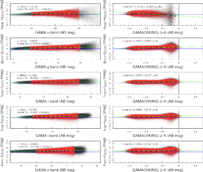
Figure 16: Comparison between SDSS PSF photometry versus SDSS (IOTA) for 420k stars. Highlighted in red are data deemed to lie in the flux and colour regions for which comparisons can be made.

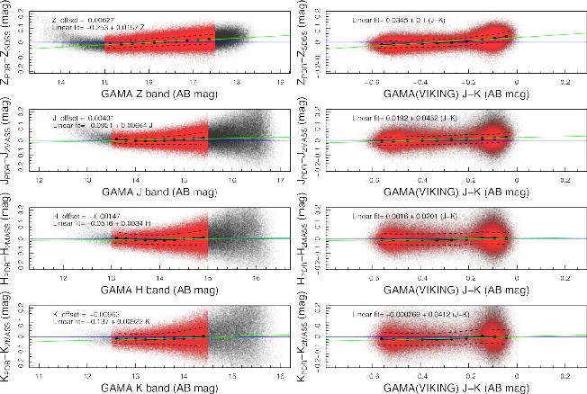
Figure 17: Comparison between 2MASS stellar photometry versus VIKING (IOTA) for 420k stars. Highlighted in red are data deemed to lie in the flux and colour regions for which comparisons can be made.

At brighter magnitudes the deeper VIKING data will suffer from saturation, and at fainter magnitudes the shallow 2MASS data will become swamped by noise. Fig. 16 and 17 show the direct comparisons (black data points), and the data which we consider robust to saturation and limiting signal-to-noise (red data points). Also shown on the figures are the derived global offset values (blue lines), and the simple linear fits (green lines) to the medians (black squares with errorbars) for both the magnitude (left) and colour comparisons (right). The dotted lines indicate the quartiles of the data.

We conclude that the absolute zero-point calibration is robust across the board to $\pm 0.02$ mag within the magnitude and colour ranges indicated (red data points). However, it is extremely important to recognise that the majority of our galaxies lie significantly outside the flux and colour ranges which we are examining here. As we shall discuss in Section 3.4 this can cause significant and intractable issues. To quantify the potential for zero-point drift between the calibration regime and operating regime we show in Table 5 possible zero-point offsets one might derive at the typical flux and the typical colour of the GAMA sample using either (a) a simple offset (Fig. 16 & 17 blue line), (b) a linear fit with magnitude (the linear fit shown as a green line in Fig. 16 & 17 left panels) and, (c) a linear fit with colour (the linear fit shown as a green line on Fig. 16 & 17 right panels). Any one of these relations, or some combination of, could be valid and hence the range reflects the uncertainty in the absolute zero-point calculations for our filters. We elect not to correct our data using any of these zero-points but instead incorporate the possible systematic zero-point error (indicated in the final column) into our analysis.

Table 5: Zero-Point uncertainties in each band.

Band	GAMA Median	GAMA Median	Potential zero-point (ZP) offsets			ZP unc.	Adopted
	flux limit (mag)	($J-K_{s}$) colour (mag)	Absolute	linear with mag	linear with colour	Mean $\pm$ Std.	ZP error
u	21.48	0.37	+0.011	+0.018	-0.020	$+0.003\pm 0.020$	0.02
g	20.30	0.40	+0.017	+0.035	+0.048	$+0.033\pm 0.016$	0.05
r	19.35	0.41	+0.018	+0.032	+0.032	$+0.027\pm 0.008$	0.03
i	18.88	0.41	+0.016	+0.033	+0.033	$+0.027\pm 0.008$	0.03
z	18.60	0.41	+0.019	+0.036	+0.035	$+0.030\pm 0.008$	0.03
Z	18.61	0.41	+0.006	+0.039	+0.076	$+0.040\pm 0.035$	0.08
Y	18.38	0.42	NA	NA	NA	NA	0.10
J	18.16	0.43	+0.004	+0.028	+0.037	$+0.023\pm 0.017$	0.04
H	17.84	0.44	-0.015	-0.050	+0.010	$-0.018\pm 0.030$	0.05
K	17.69	0.44	-0.010	+0.026	+0.018	$+0.011\pm 0.019$	0.03

3.3 $u-K_{s}$ photometry errors

Critical to any SED fitting algorithm will be the derivation of robust errors for each of our galaxies in each band. Here we derive the errors from consideration of: the zero-point error ($\sigma_{\rm ZP}$), the random sky error ($\sigma_{\rm SkyRan}$), the systematic sky error ($\sigma_{\rm SkySys}$), and the object shot noise ($\sigma_{\rm Shot}$). The first of these is quoted in Table 5, the other three can be given by:

$$\sigma_{\rm SkyRan}=\sqrt{N_{\rm Pix}}\sigma_{\rm Sky}$$ (5)

$$\sigma_{\rm SkySys}=N_{\rm Pix}\frac{\sigma_{\rm Sky}}{\sqrt{N_{\rm Aper}}}$$ (6)

$$\sigma_{\rm Shot}=\sqrt{\frac{I_{\rm Obj}}{\gamma}}$$ (7)

Where $\sigma_{\rm Sky}$ is the sky noise give in Table 3 (Col.4), $N_{\rm Pix}$ is the number of pixels in the object aperture (given by $\pi R_{\rm KRON}^{2}A_{\rm IMAGE}B_{\rm IMAGE}$ in terms of Source Extractor output parameters), and $N_{\rm Aper}$ is the number of pixels used in the aperture in which the local background was measured (i.e., $\pi R_{\rm KRON}^{2}(A_{\rm IMAGE}+32)(B_{\rm IMAGE}+32)-N_{\rm pix}$) and $\gamma$ is the gain. Of these only the gain is uncertain as during the stacking and renormalising of the data the gain is modified from its original value by varying amounts (see for example the distribution of multipliers in Fig. 5). However, as the vast majority of our galaxies are relatively low signal-to-noise detections the sky errors swamp the object shot noise errors and hence we elect to omit the object shot noise component in our final error analysis.

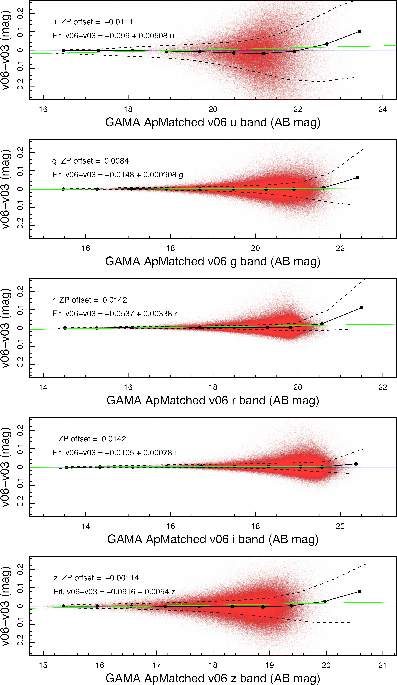
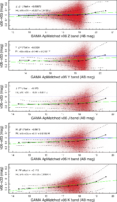
Figure 18: Comparison between GAMA ApMatchedv03 and GAMA ApMatchedv06 (i.e., PDR) $ugrizZYJHK_{s}$ galaxy photometry. Filter transformations as indicated in the text.

3.4 Comparison to earlier GAMA photometry

Finally we compare our revised SDSS+VIKING photometry to our earlier SDSS+UKIDSS photometry in Fig. 18. In this implementation of IOTA the only difference in the $ugriz$ bands is the move from a global background estimation (fixed value across the background subtracted frame) to a local background estimation. The impact appears minimal with zero-point offsets less than $\pm 0.015$. However in the $YJHK_{s}$ bands we notice significant offsets between the UKIDSS and VIKING flux measurements. The reasons for this are subtle and while they have not been exhaustively pursued we believe are most likely due a hidden linearity issue in the UKIDSS pipeline. In Fig. 19 we show our flux measurements from our UKIDSS data for 420k SDSS selected stars for which we have 2MASS photometry. The agreement is once again good, however in all cases there are significant gradients in the data and significantly stronger than those we saw in the VIKING data (r.f. Fig. 17). Extrapolating the linear fits to the flux and colour regions where the majority of our galaxies lie we infer the level of offsets seen in Fig. 18. The implication is that there may be a linearity issue with the UKIDSS calibration. Note that as Hill et al. (2010) has shown our in-house UKIDSS photometry agrees extremely well with that provided from the UKIDSS archive. We do not explore this issue further but, as a number of earlier GAMA papers are based on UKIDSS photometry, we include the UKIDSS SWarps in the public release, while cautioning against their use.

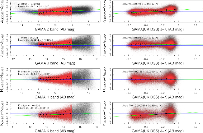
Figure 19: Comparison between 2MASS stellar photometry versus UKIDSS (IOTA) for 420k stars.

3.5 Optical motivated far-IR photometry

To derive our far-IR photometry for every GAMA target we implement an optically-motivated approach (also referred to as forced-photometry). This technique closely follows the approach developed by Bourne et al. (2012) for the Herschel-ATLAS team and which has been used to obtain SPIRE photometry at the location of known optical sources. The method adopts as its starting point the $r$-band apertures determined from our optically motivated source finding described earlier and uses the following parameter set for the apertures: right ascension, declination, major axis, minor axis and position angle. For each far-IR band the aperture defined by these parameters is combined with the appropriate PSF for each of the five bands (supplied by the Herschel-ATLAS team). The resulting 2D distribution therefore consists of a flat pedestal (within the originally defined aperture region) with edges which decline as if from the peak of the normal PSF. This soft-edge aperture can be imagined as a 2D mesa-like distribution function which can now be convolved with the data at the appropriate astrometric location. In the event of two mesas overlapping the flux is shared according to the ratio of the respective mesa functions at that pixel location, i.e., the flux is distributed using PSF and aperture information only and ignoring the intensity of the central pixel. Enhancements of this methodology are under development (Wright et al. 2015) and will include consideration of the central peak intensity along with the inclusion of interlopers (i.e., high-z targets), and iterations. The recovered fluxes at this moment contain flux from the object, plus from any low-level contaminating background objects. To assess the level of contamination we made measurements in $\sim 30,000$ apertures of comparable sizes to our object distribution which were allocated to regions where no known 5$\sigma$ Herschel-ATLAS detection exists nor any GAMA object. The mean background level in these regions was found to be zero in all SPIRE bands, as expected since the maps are made to have zero mean flux and residual large scale emission has been removed via the nebuliser step. In the PACS data small background values were found as shown in Table. 6. To correct for this effect the final step is to subtract the background values for the PACS data using the effective aperture pixel number and factoring in shared pixels where apertures overlap.

Table 6: Sky background levels per pixel as derived from blank apertures.

	Sky background (Jy)
Band	G09	G12	G15
100$\mu$m	0.0002669	0.0001491	0.0002739
160$\mu$m	0.0002044	0.0002436	0.0003784

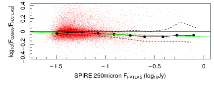
Figure 20: A comparison between the preliminary Herschel-ATLAS 5$\sigma$ catalogue and the optically motivated catalogue derived here in the SPIRE 250$\mu$m band. It should be noted that the zero-points calibration and entire reduction process have evolved between these catalogues. Note units are in Jansky as is standard in the far-IR.

Figure 20 compares our aperture-matched photometry against the Herschel-ATLAS 5$\sigma$ catalogue produced by Smith et al. (2012). In general the data agree reasonably well with offsets at the levels of 0.05dex (12%).

There have been changes in the PACS calibration and map-making algorithms between the generation of the values in the Smith et al. 2012, Rigby et al. 2011 catalogues and this work, and these changes have been substantial. Offsets at this level are consistent with these changes. For the SPIRE data, there have been no significant changes to the calibration or map-making process, however there are a number of potential issues with both the catalogues being compared in in Fig 20. Firstly, the H-ATLAS catalogue is with a preliminary version of the H-ATLAS release catalogue (Valiante et al. in prep) which does not include aperture photometry for resolved sources, explaining some of the scatter at the bright end. Secondly, the largest optical sources, which correspond to the brightest H-ATLAS sources are often shredded by SExtractor which leads to inappropriately small apertures being used for the forced photometry, and this may lead to the offset between the catalogues at the bright end and contribute to the scatter.

In Wright et al. (2015) we will compare our updated LAMBDAR photometry with the final released version of the H-ATLAS catalogue (Valiante et al. 2015) when all fluxes will be drawn from the same data pipelines and images.

3.6 Table matching the UV, optical/near-IR, mid-IR and far-IR catalogues

At this stage we have a number of distinct catalogues.

GalexMainv02: This contains measurements of the FUV and NUV fluxes which have been assembled through the use of $r$-band priors combined with curve-of-growth analysis and is described in Liske et al. (2015). We adopt the BEST photometry values. In brief the BEST photometry is that returned by the curve-of-growth method with automatic edge-detection when the NUV semi-major axis is greater than 20 arcsec or when the GAMA object does not have an unambiguous counterpart. In other cases the BEST photometry is that derived from the standard pipeline matched to the GAMA target catalogue.

ApMatchedCatv06: This contains the $u$ to $K_{s}$ band photometry as described in detail in Section 3.1

WISEPhotometryv02: as described in Cluver et al. (2014) which outlines the detailed construction of the WISE photometry with two exceptions. Firstly, for GAMA galaxies not resolved by WISE, standard aperture photometry (as provided by the AllWISE Data Release) is used instead of the profile-fit photometry (wpro). This is due to the sensitivity of WISE when observing extended, but unresolved sources, resulting in loss of flux in wpro values compared to standard aperture values (see Cluver et al. 2015 for details). Secondly, the photometry has been updated to reflect the AllWISE catalogue values. Note that this version of the catalogue also includes the correction to the updated W4 filter described in Brown, Jarrett & Cluver (2014).

HAtlasPhotomCatv01: This contains the far-IR measurements as described in Section 3.5 based on optically motivated aperture-matched measurements incorporating contamination corrections.

We use topcat to combine these catalogues by matching on GAMA CATAIDS (i.e., exact name matching), the FUV to $K_{s}$-band data are then corrected for Galactic extinction using the $E(B-V)$ values provided by Schlegel, Finkbeiner & Davis (1998; GalacticExtinctionv02) and the coefficients listed in Liske et al. (2015).

The combined catalogue is then converted from a mixture of AB mags and Janskys to Janskys throughout, with dummy values included when the object has not been surveyed in that particular band. Coverage maps may be recovered from the catalogue using the dummy values alone.

4 Robustness checks of the PDR

As the GAMA PDR is constructed from a variety of distinct catalogues and pathways it is important to assess its robustness, accuracy, and outlier rate. In earlier figures (Figs 16 to 19) we showed direct comparisons of the magnitude difference between two datasets. These are good for identifying zero-point (i.e., systematic) offsets, but not particularly useful in establishing which of the two datasets is the more robust. Here we examine the more informative “colour”-plots. The implicit assumption is that a colour distribution arises from a combination of the intrinsic colour spread of a galaxy population, convolved with the measurement error in the contributing filters. A comparison of colour-plots between two surveys, for the same sample, can provide two important statistics: the width of the distribution, and an outlier rate. The “better” quality data is the dataset with the narrowest colour range and the lowest outlier rate (assuming the zero-points are consistent). The colour-plot test is optimal when the intrinsic colour spread is sub-dominant, hence should be made using adjacent filters. In some bands, e.g., $(NUV-u)$ the intrinsic colour range is known to be broad (e.g., Robotham & Driver 2011), and hence the test less conclusive. Fig. 21 shows the full set of colour distributions for the GAMA PDR (black histograms), the data have been Galactic extinction corrected but not $k$-corrected, and this is chosen to minimise the modeling dependence, particularly given the wavelength range sampled and uncertainty in $k$-correcting certain regimes (e.g., mid-IR).

Also shown on Fig. 21 is the breadth of the colour distribution derived from the 80%-ile range (horizontal red line and red text) and the median colour value (vertical red line). We derive an outlier rate (indicated by “Out” as a percentage on the figure), this reports the percentage of galaxies which lie more then 0.5mag outside the 80 percentile range. The rationale is that the 80 percentile distribution will generally capture the intrinsic+$k$-correction spread, and a catastrophic magnitude measurement would then be one which lies more than 0.5mag outside of this range. One can see that the colour distributions are particularly broad in the UV bands (as one expects given the range from star-forming systems to inert systems with varying dust attenuation), and in the far-IR bands (as one expects given the range of dust masses and dust temperatures). The red optical and near-IR bands are the narrowest (as expected given the flatness of SEDs at these wavelengths). The outlier rates are generally highest for the poorest resolution and lowest signal-to-noise bands (i.e., $NUV$, $FUV$, $u$ and $W2$ onwards) with outlier rates varying from 12.4 percent to 0.5 percent. Our ultimate objective within the GAMA survey is to achieve outlier rates below 2 percent in all bands. With 10 colour distributions at or below this level this implies we have reached this criterion for 11 bands ($g$ to $W1$).

The facility cross-over colours, $(NUV-u)$, $(z-Z)$, $(K-W1)$, $(W4-100\mu$m), and $(160\mu$m - 250$\mu$m), are of particular interest as this is where mis-matches between objects might lead to broader distributions and higher outlier rates, and there is some indication that outlier rates do rise at these boundary points, e.g., the $(NUV-u)$ and $(z-Z)$ bands and $(K-W1)$ bands. In the case of the former this may simply reflect intrinsic+$k$-correction spread.

No dataset sampling a comparable wavelength range currently exists. However, we can compare in the optical and near-IR to the SDSS archive, our previous catalogue (based on SDSS and UKIDSS) and into the UV and mid-IR with the low-z templates given in Brown et al. (2014). These are shown where data exists as blue (GAMA ApMatchedCatv03; SDSS+UKIDSS), green (SDSS DR7 ModelMags), and purple histograms (Brown et al.). Note that as the SDSS and GAMA data are essentially derived from the same base optical data and it is the photometric measurement method which is being tested here. In future we will be able to compare to KiDS and Subaru HSC datasets. In comparison to our previous GAMA catalogue we can see that PDR represents an improvement (lower breadths and lower outlier rates) in all bands. In particular the near-IR bands are significantly improved with the colour spread now at least two times narrower. This reflects the greater depth of the VIKING data over the UKIDSS LAS data (see Table 3). In comparison to SDSS DR7 ModelMags we can see that GAMA PDR appears to do marginally better in the $(u-g)$ and $(g-r)$ colours, but marginally poorer in the $(r-i)$ and $(i-z)$ bands, in all cases by modest amounts.

Finally, in comparison to the colour distributions derived from the Brown et al. (2014) templates there are two important caveats. Firstly the Brown data makes no attempt to be statistically representative but rather provides an indication of the range of SEDs seen in the nearby population for a relatively ad hoc sample. Secondly the GAMA PDR has a median redshift of $z=0.24$ and in some bands the k-correction will dominate over the intrinsic distribution. This is apparent in particular in the $(NUV-u)$, $(u-g)$ and $(g-r)$ bands where the 4000Å break is redshifted through. This results in significantly broader colours in the observed GAMA PDR colour distributions not seen in the rest-frame templates. Again this is understandable. More puzzling is the converse where the $(W2-W3)$ and $(W3-W4)$ distributions which are clearly broader in the Brown et al data. This may reflect the incompleteness within the GAMA PDR in these bands, with the bluest objects perhaps being detected in W2 but not in W3, and hence not represented on these plots (see Cluver et al. 2014 for full discussion on the WISE completeness). Similarly for $(W3-W4)$. For example the Brown et al., sample includes both Elliptical systems and very low luminosity blue dwarf systems (e.g., Mrk 331, II Zw 96, Mrk 1490, and UM 461) neither of which would be likely detected by WISE at $z>>0.01$. The obvious solution is to derive “forced-photometry” for the full GAMA input catalogue across all bands.

At this point we believe we have established that GAMA PDR is matching SDSS DR7 ModelMags, a significant improvement over previous GAMA work based on SDSS+UKIDSS LAS, but there remains some concerns regarding higher than desired outlier rates in the lower signal-to-noise and poorer resolution bands, and the need for a measurement at the location of every GAMA galaxy regardless of whether there is obvious flux or not (i.e., forced photometry). Fixing these problems is non-trivial and requires dedicated panchromatic software, which is currently nearing completion and will be presented in Wright et al. (2015).

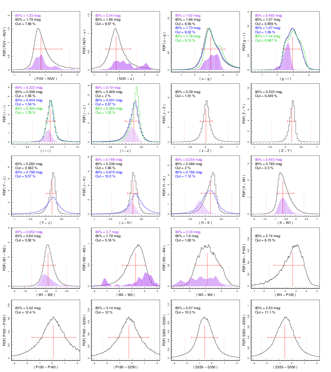
Figure 21: Each panel shows a histogram of a GAMA PDR colour histogram (black distribution) from two adjacent filters (as indicated, y-axis). The horizontal red bar indicates the 80-percentile range of the data with the value for GAMA PDR indicated in black in the top left corner. The outlier rate (indicated by Out) reports the percentage of the distribution which lies $>$0.5mag outside the 80-percentile range (indicated by the vertical dotted lines). Where possible we overlay data from the SDSS DR7 (ModelMag colours, green histograms) and ApMatchedCatv03 (which uses SDSS and UKIDSS data, blue histograms). All distributions are extinction corrected but otherwise as observed. Finally the shaded histogram (purple) shows data from the $z=0$ sample of Brown et al. (2014). However, note that the Brown sample has an ad hoc selection and essentially represent k-band corrected data - hence explaining the apparent discrepancy in $(NUV-u)$, $(u-g)$ and $(g-r)$, and $(H-K)$.

4.1 Composite SEDs

Using a 35,712 core machine available at the Pawsey Supercomputing Centre Facility (MAGNUS) we have now run the MAGPHYS spectral energy distribution fitting code (de Cunha, Charlot & Elbaz 2008), over the full equatorial GAMA sample with redshifts, i.e., 197k galaxies (using the Bruzual & Charlot 2003 spectral synthesis model). MAGPHYS takes as its input, flux measurements in each band, associated errors, and the filter bandpasses, and returns the attenuated and unattenuated SED models from FUV to far-IR, along with a number of physical measurements, e.g., stellar mass, star-formation rate, dust mass, dust opacity, dust temperatures (birth-cloud and ISM) etc (for more details please see da Cunha et al. 2008). Here we look to use MAGPHYS to provide a simple spectral energy representation for each of our galaxies which also has the effect of filling in the gaps where coverage in a particular band does not exist or no detection is measured. On a single processor MAGPHYS will typically take 10mins to run for a single galaxy (i.e., 4yrs for our full sample), but using MAGNUS the entire sample can be processed in less than 24hrs.

Fig. 22 shows each of the $21\times 197,491$ datapoints plotted at the rest wavelength versus the number of $\sigma$ deviations the GAMA PDR magnitude is away from the derived MAGPHYS magnitude. The figure highlights that generally MAGPHYS appears to be finding consistent fits across all bands with only the W4 showing some indication of a fundamental inconsistency between the data and the models. This has now been tracked down to the change in the W4 filter transmission curve with our MAGPHYS run still using the old throughput curve while the WISE PDR data uses the revised W4 transmission curve (see Brown, Jarrett & Cluver 2014 for full details). Future runs of MAGPHYS will use the updated curve. The distribution of the data points in $\sigma$ deviations (abscissa) suggest that the measurement variations are consistent with the errors quoted. The bleed of the far-IR data to the lower part of the figure, is most likely due to contamination by high-z systems (as expected). In the wavelength range, within each filter the near-IR data shows the most fluctuations. These are likely to reflect recurrent features in the MAGPHYS models shifting through the various bands and suggests some uncertainty in the precise modelling of the TP-AGB region as noted by numerous groups, e.g., Maraston et al. (2006).

Fig. 23 shows the MAGPHYS SED model fits sampled by our $z<0.06$ morphologically classified sample, separated into E/S0s (red), Sabcs (green) or Sd/Irrs (blue). See Moffett et al. (2015) for details on the sample and morphological classification process. In order to construct these plots the individual SEDs derived by MAGPHYS have been normalised to the same stellar mass, i.e., their SEDs have been scaled by their fractional stellar mass offset from $10^{10}M_{*}$ (using the stellar masses derived by MAGPHYS). The curves shown are the quantile distributions for 10, 25, 45, 50, 55, 75 and 90 percent as a function of wavelength. Note that these do not represent individual MAGPHYS SED models, but are quantile ranges in narrow wavelength intervals which are then linked to create the SED quantiles - hence the SEDs show more variations than the models used in MAGPHYS if examined in detail. The reason for this representation is to avoid a specific calibration wavelength and SEDs that, when calibrated into quantiles at one wavelength, cross at others.

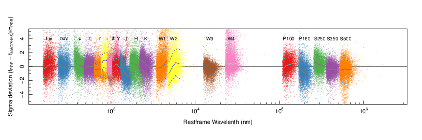
Figure 22: Sigma deviations of the model photometry compared to the input photometry versus rest wavelength for all data points for all galaxies. For each colour the median and 1$\sigma$ dispersions is measured and shown (grey solid and dotted lines respectively). The plot shows that the majority of our data lies within the quoted error of the MAGPHYS fits with some outliers (as also noted in Fig. 21). The offset of W4 is of some concern as is the bleeding of the far-IR data towards negative deviation values. Both of these effects are believed to be understood but requires the LAMBDAR software (in development). If these are flat and offset it implies a systematic offset, if they show trends with wavelength it implies a progression of a feature with redshift. Trends are most apparent in the near-IR where the modelling of the TP-AGB population is still uncertain.

Fig. 23 illustrates not only the wealth of data provided by the GAMA PDR but a number of physical phenomena. Firstly the spread at any wavelength point represents the mass-to-light ratio at that wavelength. This can be seen to be narrowest in the 2 - 5$\mu$m range (as expected), indicating that this region is optimal for single band stellar-mass estimates. However, the constant gradient in this region implies that near-IR colours provide little further leverage to improve the stellar-mass estimation beyond single band measurements. Conversely the smooth variation of SED gradients in the optical from low to high stellar-mass ratios, imply that optimal stellar-mass estimation may arise from the combination of a single band near-IR measurement combined with an optical colour (see also discussion in Taylor et al. 2011). Fig. 23 highlights the known strong correlations between UV flux, far-IR emission and stellar mass-to-light ratio with all being amplified or suppressed in Sd/Irrs or E/S0s respectively. However, that all galaxies seem to contain some far-IR emission may be a manifestation of the MAGPHYS code tending to maximise dust content within the bounds as allowed by the far-IR errors. Curiously the Sabc (green) provide a very narrow range of parameters, perhaps indicating a close coupling between star-formation, dust production, and the mass-to-light ratio — arguably indicative of well-balanced self-regulated disk formation/evolution. The greater spreads in the early (red) and later (blue) types are perhaps indicative of the progression through various stages of quenching (ramping down) and unstable disc formation (overshoot) respectively. In particular Agius et al. (2015) found an unexpectedly high levels of dust in a significant (29%) population of the GAMA-E/S0 galaxies consistent with a range of E-So SEDS. Note also the results presented on observed correlations between the star-formation rate, specific star-formation rate in da Cunha et al. (2010) and Smith et al. (2012); see also interpretation in Hjorth et al. (2014). A detailed exploration of these phenomena are beyond the scope of this paper but the potential is clear particularly in conjunction with the existing group (Robotham et al. 2011) and large scale structure (Alpaslan et al. 2014) catalogues.

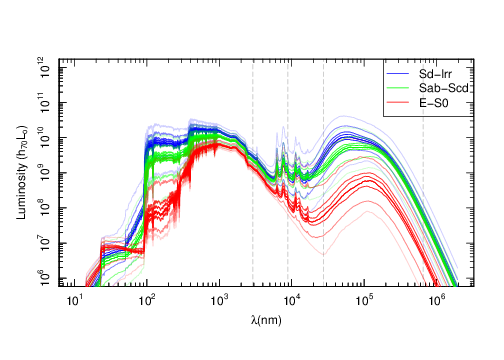
Figure 23: The panel shows the 10, 25 ,45 ,50 ,55 ,75 and 90 percentiles for the full GAMA PDR SEDs for the $z<0.06$ morphologically classified sample presented in Moffett et al. (2015). The data are initially scaled to the same mass and then at each wavelength point the quantiles derived which then collectively trace out the quantiles over wavelength. The spread at each wavelength therefore directly reflects the spread in the mass-to-light ratio at that wavelength.

4.1.1 Inspection of individual objects

We explore individual SEDs for one hundred systems randomly selected (IDs 47500-47609). Approximately 5-10 percent are found to have one or more significant outlier(s) in the photometry but otherwise good MAGPHYS fits are found for all 100 systems. In approximately 50 percent of cases the far-IR photometry is essentially missing (due to the shallowness of the far-IR data), hence flux and/or redshift cuts are advisable depending on the science investigation to be conducted. Fig. 24 shows four example galaxies which include a nearby bright system (G47152, $z=0.082$), a nearby faint system (G47157, $z=0.074$), a higher redshift crowded system (G47609, $z=0.282$), and a known far-IR lens system (G622892, $z=0.300$; Negrello et al. 2010; recently shown to exhibit a spectacular Einstein ring, the very high far-IR flux is evident). The panels on the left show the combined $giH$ colour image from a combination of VIKING and SDSS data. Overlaid (green dotted lines) are apertures for the main object and nearby systems in our bright catalogue. The right panels show the 21-band measured photometry (green data and errorbars) in units of total energy output ($\lambda L_{\lambda}$ in units of h₇₀ W) at the filter pivot-wavelength divided by $(1+z)$ (i.e., rest wavelength). The red and blue lines show the attenuated and unattenuated SEDs from the preliminary MAGPHYS fits. Purple circles show the flux from the attenuated SED curve integrated within the filter bandpasses given in Fig. 1. The lower portion of the panel shows the residuals expressed as the ratio of the observed flux to the measured flux. Included in the error budget is a 10 percent flux component added in quadrature to mitigate small systematic zero-point offsets at facility boundaries. Comparable plots for all 221k systems with redshifts are provided via the GAMA $\Psi$ online cutout tool (http://gama-psi.icrar.org/)

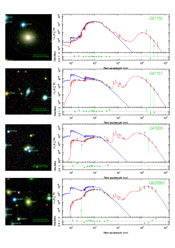
Figure 24: Four example galaxies from the GAMA PDR showing, in each case, the $Hig$ image with the apertures overlaid, and the 21-band photometry with the attenuated (red) and unattenuated (blue) MAGPHYS fits to the data. Data shown in green represent the measured photometry plotted at rest wavelength while the purple circles show the integrated flux measured from the attenuated MAGPHYS fit through the appropriate filter. The lower portion of the main panels shows the residuals, i.e., the ratio of the observed flux to the model flux. Errors include an arbitrary 10 percent error added in quadrature intended to incorporate some allowance for zero-point offsets between facilities. Note that the lowest image is a well known lens system reported by Negrello et al. (2010). All images are derived from the GAMA $\Psi$ online cutout tool http://gama-psi.icrar.org/

The four galaxies are each well sampled by the GAMA PDR data which collectively map out the two key peaks in the energy output due to starlight and dust reprocessing of starlight. The four systems also show varying degrees of dust attenuation with the observed fluxes requiring minimal, significant and extreme corrections to recover the unattenuated fluxes. In all cases the residuals are well behaved, given the errors. Exploring the GAMA PDR more generally, the SED data appear robust with catastrophic failures in one band typically at the levels indicated in Fig. 21, i.e., 10 percent in poorly-resolved bands to 1 percent in well-resolved bands. Obvious issues which arise following inspection of several hundred SEDs are: incorrect apertures, data artifacts (i.e., poor quality regions), nearby bright stars (diffraction spikes and blocking), crowding, and confusion.

5 The energy output of the Universe at $z<0.2$ from FUV to far-IR

We conclude this paper with a brief look at the integrated energy output of the low redshift galaxy population, i.e., the Cosmic Spectral Energy Distribution (CSED), its recent evolution, and the implied integrated photon escape fraction. The CSED represents the energy output of a cosmologically representative volume, in essence an inventory of the photons recently generated, as opposed to those passing through but formed earlier. It can be reported both pre- and post- attenuation by the dust content of the galaxy population, both are interesting. The pre-attenuated CSED informs us of the photons being created from (primarily) nucleosynthesis processes (in the current epoch), while the post-attenuated CSED informs us of the photons entering into the IGM. The sum of the two must equal (energy conservation), but the wavelength distribution will differ as dust re-processes the emergent photons from short (UV and optical) to long (mainly far-IR) wavelengths. The combination of the two can be used to determine the integrated photon escape fraction. By integrated we imply over a representative galaxy population, and averaged over representative viewing angles. Both of these factors are important and make the integrated photon escape fraction useful for converting observed FUV and NUV fluxes to robust star-formation rates. The work follows earlier measurements of the CSED reported in Driver et al. (2008) and Driver et al. (2012). However, the methodology here is very different and for the first time includes mid- and far-IR data in a fully consistent analysis. In our earlier studies we determined luminosity distributions in each band independently and then fitted across these values to determine the CSED. Here we stack the individual MAGPHYS SEDs fits derived earlier, as representative fitting functions (see Fig. 24).

Potentially, as we have a MAGPHYS fit for every galaxy we could use them to derive fluxes in data gaps and use the full sample. However, given the critical importance of the far-IR dust constraint we elect to use just the common region with full 21-band coverage (see Figs. A27 to A30). This combined region constitutes an area of 63 percent of the full area or 113 deg² and contains 138k objects with secure redshifts in the range $0.02<z<0.5$ (trimmed to exclude stars and high-z AGN). To explore any evolution of the CSED, we divide our sample into three redshift intervals: $0.02<z<0.08$, $0.08<z<0.14$ and $0.14<z<0.2$ which correspond roughly to lookback times of 0.8 Gyr, 1.5 Gyr and 2.25 Gyr respectively. The volumes sampled are: $4.9\times 10^{5}$, $2.1\times 10^{6}$ & $4.6\times 10^{6}$ h${}_{70}^{-3}$ Mpc³ respectively (factoring in our reduced coverage). Within each redshift range we use the $z_{\rm max}$ values reported in Taylor et al. (2011) to derive a weight as not all galaxies would be visible across the selected redshift range. Galaxies with $z_{\rm max}$ values above the redshift range have weights set to unity, and values with $z_{\rm max}$ below this range have weights set to zero. Otherwise weights are set to the inverse of the fraction of the volume sampled. A cap is placed ensuring no weight exceeds a value of 10, this ensures a single lone system just fortuitously within the redshift range cannot dominate the final outcome by being massively amplified. Within each redshift range we now simply sum the energy $\times$ weight (i.e., $\sum W_{i}\lambda L^{i}_{\lambda}$) for the galaxies within our selection to arrive out the CSED for that volume.

These raw derived CSEDs require one final correction to accommodate for the loss of lower luminosity systems in the higher redshift bins. To determine the correction factor we repeat the summation but with a stellar mass cut imposed on all three samples ($10^{10}$M_⊙), this is sufficiently low to be sampling the dominant contribution to the CSED but not so low as to suffer total incompleteness (i.e., that which is not corrected for by our weights). For each volume interval we obtain unrestricted to mass-restricted CSED ratios of: 1.68, 1.48 and 1.29 for the low, mid, and high redshift samples respectively. If all three samples were complete this ratio would be constant, hence this changing ratio encodes the loss of the lower luminosity systems in the higher redshift bins, and can therefore be used to provide an appropriate correction. This is achieved by scaling the final CSED curves by factors of 1.00, 1.14 (i.e., 1.68/1.48), and 1.30 (i.e., 1.68/1.29) respectively. In effect we are using the CSED shape from the unrestricted samples but normalising using the restricted samples and this is analogous to the normalisations typically used in estimating luminosity and mass functions. This implicitly assumes the following: that the low redshift sample is itself complete (hence requiring no scaling), and that the ratio of energy emerging from systems above and below $10^{10}$M_⊙ is approximately constant. The first of these is relatively secure: GAMA is a deep survey and at $z\sim 0.08$ is mass complete to $10^{9}$M_⊙ (see Lange et al. 2015), below which there is very little contribution to the luminosity density (see Driver 1999), or stellar mass density (see Moffett et al. 2015). In the second case we understand low-mass systems are preferentially star-forming and may have evolved more rapidly over recent times compared to the more massive systems. However, as the correction factors are relatively modest (14 percent and 30 percent) the shape and renormalisation is unlikely to be dramatically changed, but we acknowledge may be biased low. This can only be quantified through deeper studies (see for exampled the planned WAVES survey; Driver et al. 2015).

Fig. 25 shows the resulting energy outputs for the renormalised unattenuated CSED (upper) and the renormalised attenuated CSED (lower) with the redshift ranges represented by colour as indicated. Also shown is our earlier estimate derived from GAMA via luminosity function fitting (orange line). It is worth re-iterating that the Driver et al. (2012) CSED measurement is based on luminosity density measurements from $FUV$ to $K_{s}$ combined with an adopted integrated photon escape fraction (Driver et al. 2008) to infer the mid and far-IR portion, i.e., the mid and far-IR from Driver et al. (2012) is a prediction, and hence shown as a dotted line beyond $2.1\mu$m. Also shown is the prediction from semi-analytic modelling by Somerville et al. (2012). Both curves, corrected to $H_{o}=70$ km/s/Mpc, follow the new low-z CSED very well in the optical and start to diverge in the mid and far-IR bands where previous empirical data have been lacking. The Somerville curve, in particular traces the low-redshift bin extremely well with the previous Driver data significantly under-predicting the far-IR emission. The CSEDs presented here represent a major advance constituting the first consistent measurement of the post- attenuated CSED from a single sample spanning from the $FUV$ to far-IR. Hence, while cosmic (sample) variance (CV) may scale the respective CSEDs in overall density, it will not modify the shape of the distribution (unless there are extreme hidden clustering factors). Using the formula in Driver & Robotham (2010, see also the online calculator http://cosmocalc.icrar.org/) we derive the CV, for our three redshift ranges to be: 18 percent, 12 percent and 10 percent respectively, with increasing redshift and note that despite the extent of the GAMA PDR the dominant error remains the CV.

To first order the CSEDs are therefore all consistent with each other and the previous values. The CSEDs follow the expected progression towards higher energy output towards higher redshifts, despite the potential uncertainty in overall normalisation from CV. In particular the far-IR increases noticeably faster than the optical. This result is independent of cosmic variance and noted previously within the far-IR community, see for example Dunne et al. (2011) who infer a significant increase in dust mass (towards high redshift) over the past 5 Gyr. In detail we can report that the Universe is in energy decline, having dropped from a total energy production of $(2.5\pm 0.2)\times 10^{35}$ h₇₀ W Mpc^-3 at 2.25 Gyr ago, to $(2.2\pm 0.2)\times 10^{35}$ h₇₀ W Mpc^-3 1.5 Gyr ago and $(1.5\pm 0.3)\times 10^{35}$ h₇₀ W Mpc^-3 0.75 Gyr ago. This decline is significant despite the CV uncertainty, and in line with our understanding of the evolution in the cosmic star-formation history (e.g., Hopkins & Beacom 2006), which shows a decline of a factor of approximately $\times 1.5$ over this time-frame. The lowest redshift bin value is also consistent with the $(1.26\pm 0.09)\times 10^{35}$ h₇₀ W Mpc^-3 for $z<0.1$ as reported in Driver et al. (2012) and the orange and blue curves on Fig. 25 do show consistency over the optical regime. The majority of the energy difference is derived from the far-IR where previous data was lacking and the CSED in this region estimated. As an aside it is also worth noting that the near-IR data show some slight disagreement, and this is consistent with our finding that VIKING fluxes are typically brighter than UKIDSS LAS fluxes (see Section 3.4). Finally, shown on Fig. 25 are the SPIRE data points derived by the Herschel-ATLAS team from the initial data release which sampled all of G09, G15 and half of G12 (Bourne et al. 2012). These data are low compared to our new estimate, however the SPIRE calibration and data reduction have evolved quite substantially since these data-points were derived.

Integrating these distributions reveals some interesting numbers. From the unattenuated CSED we find that 50 percent of the energy production in the nearby Universe is at wavelengths in the range 0.01—0.64$\mu$m (i.e., UV/optical). In the post-attenuated “observed” CSED, 50 percent of the energy emerges at wavelengths shorter than 1.7$\mu$m. Splitting at 10$\mu$m we find that 65 percent of the energy produced (via stellar emission) is released into the IGM at shorter wavelengths and 35 percent at longer wavelengths. Despite dust contributing a very small proportion of a galaxy’s mass (typically $<1$ percent; Driver et al. 2008), its impact on the energy output is dramatic with significant potential consequences for optically based flux and size measurements (see for example Pastrav et al. 2013).

Dividing the pre- and post-attenuated CSEDs yields the integrated photon escape fraction (IPEF). This is a particularly interesting distribution as it encapsulates the impact of dust in a simple and general way. Fig. 26 shows the IPEF in the three redshift bins. Also shown (purple diamonds) is the IPEF derived in Driver et al. (2008) for the Millennium Galaxy Catalogue (Liske et al. 2003). Clearly apparent is a trend towards lower photon escape fractions towards modestly higher redshift, demonstrating the impact of dust evolution in our perception of even low redshift systems ($z<0.2$). It is important to note that this result is resilient to CV as we are comparing the ratio of the pre- and post- attenuated CSEDs and hence the normalisation cancels out. The variation appears smooth with redshift and significant, with the escape fraction in the FUV changing from 18 percent in the higher redshift bin to 23 percent in the lower z bin. The corresponding change in the NUV is 27 percent to 34 percent respectively. If this trend continues the implication is that at even intermediate redshifts the UV photon escape fraction may be significantly lower than the values typically adopted when deriving star-formation rates from UV fluxes.

The above work should be considered as preliminary, but indicative of the potential of the GAMA PDR to explore the energy outputs of galaxies and galaxy population at low redshift. The analysis at present also includes a number of important caveats which we are looking to address in the near future. The first is out-standing issues related to the GAMA photometry: aperture robustness, the need for a uniform forced photometry across all bands, and improved management of the variable spatial resolutions and signal-to-noise limits. The second is whether MAGPHYS provides truly unbiased fits, particularly in the far-IR where our data quality is lowest and where, as the errors grow, over-fitting of the far-IR fluxes cannot be ruled out. Verifying that MAGPHYS is unbiased will be important as our data quality undoubtedly declines with redshift. One should also bear in mind that the interpretations above are very much based on the assumptions embedded in the MAGPHYS code, in due course it will be important to explore a range of assumptions and to undertake critical comparisons against fully radiative-transfer codes for well-resolved systems. The third and arguably most fundamental issue relates back to the integrity of the GAMA input catalogue and in particular its reliance on the fairly shallow SDSS imaging and the potential for missing extended low surface brightness systems. The GAMA regions are currently being surveyed by the VST KiDS team and will also be surveyed as part of the HSC Wide survey, both datasets can be used to improve our input catalogue particularly for extended low surface brightness systems.

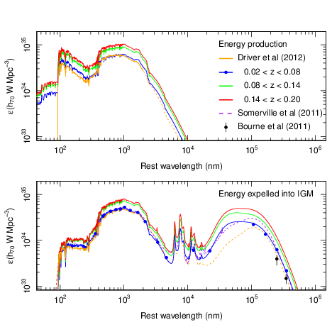
Figure 25: The energy originating (i.e., unattenuated, top), and emanating (i.e., attenuated following dust reprocessing, lower) at intervals equivalent to 0.75, 1.5 and 2.25 Gyr lookback time. The data are normalised to the energy output per Mpc³ for $H_{o}=70$km/s/Mpc. The data show clear trends in the evolution of the total energy output over this timeline.

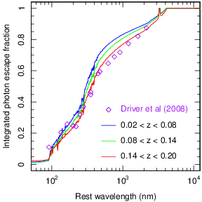
Figure 26: The photon escape fraction integrated over all viewing angles and derived from Fig. 25. Also shown is the escape fraction reported by Driver et al. (2008) from the Millennium Galaxy Catalogue within the redshift range $0.0<z<0.18$. The data show a clear progression towards lower escape fractions as redshift increases.

6 Summary

We have brought together a number of diverse datasets from three space missions (GALEX, WISE and Herschel), and two ground-based facilities (SDSS and VISTA) to produce the GAMA Panchromatic Data Release. The individual dataframes have been astrometrically and photometrically matched, and then SWarped into single images for each of the three equatorial GAMA regions covering 80 deg² each (i.e., slightly larger than the nominal 60 deg² region covered by the spectroscopy). Weight maps are provided indicating the number of frames contributing to each region and files containing the names of the individual frames used. In the $u-K_{s}$ bands we provide both native resolution data and data degraded to a common 2^′′ full-width half maximum. The SWarped images along with a cutout tool (GAMA $\Psi$) for extracting subregions are available at:

http://gama-psi.icrar.org/

Note that the Herschel data is currently proprietary but will be made available following the Herschel-ATLAS final data release.

GAMA $\Psi$ also provides additional functionality to create colour images on the fly from the combination of any of the 21-bands, individual fits downloads, object and aperture overlays and is maintained by the International Centre for Radio Astronomy Research (ICRAR) Data Intensive Astronomy (DIA) unit. Queries and comments on GAMA $\Psi$ should be sent to simon.driver@uwa.edu.au.

We describe the construction of the $u-K_{s}$ aperture-matched photometry following the method described in Hill et al. (2011) and compare to our previous measurements. In addition we compare our near-IR photometry for 400k stars extracted from 2MASS and confirm that our zero-points are robust to within a tenth of a magnitude.

The VIKING-2MASS and UKIDSS-2MASS zero-points are shown to be robust however VIKING-UKIDSS photometry do not agree. This apparent tautological inconsistency is most likely explained by a linearity issue as the VIKING and UKIDSS data are compared at a significantly fainter magnitude range. Some evidence is seen for a linearity issue in the UKIDSS-2MASS comparison, which when extrapolated to fainter magnitudes does appear to explain the offsets seen between VIKING and UKIDSS.

We also describe our method for deriving far-IR measurements using optical priors where we use our $r$-band apertures convolved with the appropriate instrument/filter PSF to measure the far-IR flux at the location of every object.

We then combine our $u-K_{s}$ and $100-500\mu$m fluxes with GALEX and WISE data derived by the MPIK and UCT/UWC groups led by RJT and MC using exact name ID matching. This results in a final catalogue of over 221k objects from the G09, G12, G15 and G23 regions, 63 percent of which have complete coverage in all 21 bands.

Finally as a demonstration of this dataset we derive the total flux originating and emanating from various volumes from FUV to far-IR at redshifts indicative of 0.8, 1.5 and 2.25 Gyr lookback time. We see evidence for evolution over this period consistent with the decline of star-formation traced by the cosmic star-formation history and consistent with the reported evolution of the far-IR luminosity functions.

In future papers we will further improve our flux extraction method using optically motivated priors in all bands, leading to more consistent errors, and explore the physical properties derived from SED fitting codes for various populations and sub-populations.

References

Abazajian K.N., et al., 2009, ApJS, 182, 543

Agius N., et al., 2015, MNRAS, in press (arXiv:1505.06947)

Alpaslan M., et al., 2014, 438, 177

Andrae E., 2014, PhD Thesis, MPIfK

Arnaboldi M., et al., 2007, Messenger, 127, 28

Baldry, I.K., et al., 2010, MNRAS, 404, 86

Barnes D.G., et al., 2001, MNRAS, 322, 486

Bate, M, Bonnell, I.A., Bromm, V., 2003, MNRAS, 339, 577

Bertin E., 2010, Astrophysics Source Code Library, record ascl.1010.068

Bertin E., 2011, ASPC, 442, 435

Bourne N., et al., 2012, MNRAS, 421, 3027

Brown M.J.I., Moustakas J., Smith J.D.T., da Cunha E., Jarrett T.H., Imanishi M., Armus L., Brandl B.R., & Peek J.E.G., 2014, ApJS, 212, 18

Brown M.J.I., Jarrett T.H., Cluver M.E., 2014, PASA, 31, 49

Bruzual G., Charlot S., 2003, MNRAS, 344, 1000

Calzetti D., Armus L., Bohlin R.C., Kinney A.L., Koornneef J., Storichi-Bergmann T., et al., 2000, ApJ, 533, 682

Cluver M., et al., 2014, ApJ, 782, 90

Cluver M., et al., 2015, MNRAS, in preparation

da Cunha E., Charlot, S., Elbaz D., 2008, MNRAS, 388, 1595

da Cunha E., Eminian C., Charlot, S, Blaizot J., 2010, MNRAS, 403, 1894

Dalton G., et al., 2006, SPIE, 6269

de Jong J.T.A., Verdoes Kleijn, G.A., Konrad, K.H., Valentijn E.A., 2013 Experimental Astronomy, 35, 25

Drinkwater M.J., et al., 2010, MNRAS, 401, 1429

Driver S.P., 1999, ApJ, 526, 69

Driver S.P., et al., 2007, MNRAS, 379, 1022

Driver S.P., et al., 2009, A&G, 50, 12

Driver S.P., et al., 2008, ApJ, 678, 101

Driver S.P., et al., 2011, MNRAS, 413, 971

Driver S.P., et al., 2012, MNRAS, 427, 3244

Driver S.P., Davies L.J., Meyer M., Power C., Robotham A.S.G., Baldry I.K., Liske J., Norberg P., 2015, ASSP, in press (arXiv: 1507.00676)

Domínguez A., et al., 2011, MNRAS, 410, 2556

Dunne L., et al., 2011, MNRAS, 417, 1510

Eales S. et al., 2010, PASP, 122, 499

Edge A., Sutherland W., Kuijken K., Driver S.P., McMahon R., Eales S., Emerson J.P., 2013, Messenger, 154, 32

Fontanot F., Monaco P., Cristiano S., Tozzi P., 2006m MNRAS, 373, 1173

Giavalisco M., et al., 2004, ApJ, 600, 93

Griffin M.J., et al., 2010, A&A, 518, 232

Grogin N.A., et al., 2011, ApJS, 197, 35

Hill D., et al., 2010, MNRAS, 404, 1215

Hill, D., et al., 2011, MNRAS, 412, 765

Hambly N.C., et al., 2001, MNRAS, 326, 1279

Hjorth J., Gall C., Michalowski M.J., 2014, MNRAS, 782, 23

Hopkins A.M., et al., 2013, MNRAS, 430, 2047

Hopkins A.M., Beacom J.F., 2006, ApJ, 651, 142

Hopkins P.F., Hernquist L, Cos T.J, Di Matteo T, Robertson B, Springel, V, 2006, ApJS, 163, 1

Ibar E., et al., 2010, MNRAS, 409, 38

Jarrett T.H., et al., 2012, AJ, 144, 68

Jarrett T.H., et al., 2013, AJ, 145, 6

Kelvin L., et al., 2012, MNRAS, 421, 1007

Kelvin L., et al., 2014, MNRAS, 444, 1647

Kennicutt R.C., et al., 2003, PASP. 115, 928

Keres D., Katz N, Weinberg D, Davé R., 2005, MNRAS, 363, 2

Koekemoer A.M., et al., 2011, ApJS, 197, 36

Komatsu E., et al., 2011, ApJS, 192, 18

Lacey C., Cole S., 1993, MNRAS, 262, 627

Lange R., et al., 2015, MNRAS, 447, 2603

Lewis J.R., Irwin M., Bunclark P., 2010, ASPC, 434, 91

Liske J., et al., 2003, MNRAS, 344, 307

Liske J., et al., 2015, MNRAS, 452, 2087

Maddox S.J., et al., 2015, MNRAS, in preparation

Maraston C., Daddi E., Renzini A., Cimatti A., Dickinson M., Papovich C., Pasquali A., Pirzkal N., 2006, ApJ, 652, 82

Martin C., et al., 2005, ApJ, 619, 1

Masci F.J., 2013, online only, arXiv:1301.2718

Masci F.J., Fowler J.W., 2009, ASPC, 411, 67

McKee C.F., Ostriker E.C., 2007, ARA&A, 45, 565

Moffett A., et al., 2015, MNRAS, submitted

Morrissey P., et al., 2007, ApJS, 173, 682

Munoz-Mateos J.C., et al., ApJS, in press (arXiv:1505.03534)

Negrello et al., 2010, Science, 330, 800

Pascale E., et al., 2011, MNRAS, 415, 911

Pastrav B., Popescu C.C., Tuffs R.J., Sansom A.E., 2013, A&A, 557, 137

Pilbratt G.L., et al., 2010, A&A, 518, 1

Poglitsch A., et al., 2010, A&A, 518, 2

Popescu C.C., Tuffs R.J., 2002, MNRAS, 335, 41

Rigby E.E., et al., 2011, MNRAS, 415, 2336

Robotham A.S.G., Driver S.P., 2011, MNRAS, 413, 2570

Robotham A.S.G., et al., 2011, MNRAS, 416, 2640

Robotham A.S.G., et al., 2010, PASA, 27, 76

Rowlands K., et al., 2012, MNRAS, 419, 2545

Schlegel D.J., Finkbeiner D.P., Davis M., 1998, ApJ, 500, 525

Schoenberner D., 1983, ApJ, 272, 708

Scoville, N., et al., 2007, ApJS, 172, 1

Sheth K., et al., 2010, PASP, 122, 1397

Shu F., Adams F.C., Lizano S., 1987, ARA&A, 25, 23

Skrutskie M.F., et al., 2006, AJ, 131, 1163

Smith D., et al., 2011, MNRAS, 416, 857

Smith D., et al., 2012, MNRAS, 427, 703

Somerville R., Gilmore, R.C., Primack J.R., Domínquez A., 2012, MNRAS, 423, 1992

Soto M., et al., 2013, A&A, 552, 101

Soifer B.T, Neugenbauer G., Hoick J.R., 1987, ARA&A, 25, 187

Sutherland R., et al., 2015, A&A, 575, 25

Tuffs R.J., Popescu C.C., Völk H.J., Kylafis N.D., Dopita M.A., 2004, A&A, 419, 821

Taylor, N., et al., 2011, MNRAS, 418, 1587

Toomre A., & Toomre J., 1972, ApJ, 178, 623

Tinsley B., 1980, Fund. Cosmic Physics, 5, 287

Valiante E., et al., 2015, MNRAS, in preparation

Veilleux S., Cecil G., Bland-Hawthorn J., 2005, ARA&A, 43, 769

White R.L., Becker R.H., Helfand D.J., Gregg M.D., 1997, ApJ, 475, 479

White S.D.M., Rees M.J., 1978, MNRAS, 183, 341

Wright A., et al., 2015, MNRAS, in preparation

Wright E.L., et al., 2010, AJ, 140,1868

York D., et al., 2000, AJ, 120, 1579

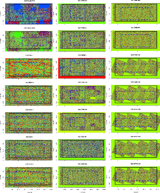
Figure 27: Background uniformity and coverage in the G09 region for GALEX, SDSS, VIKING, WISE and Herschel data. The black box denotes the GAMA spectroscopic survey region and the blue box the region from which the background statistics were derived. We use the MOGRIFY package to display the low-res data frames very close to the sky level. Astronomical objects will not be visible, however the frames highlight the coverage, missing regions, and the integrity of the large scale sky structure.

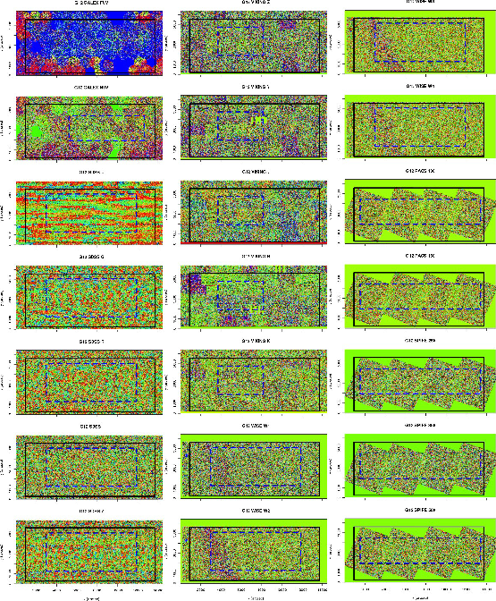
Figure 28: Background uniformity and coverage in the G12 region for GALEX, SDSS, VIKING, WISE and Herschel data.

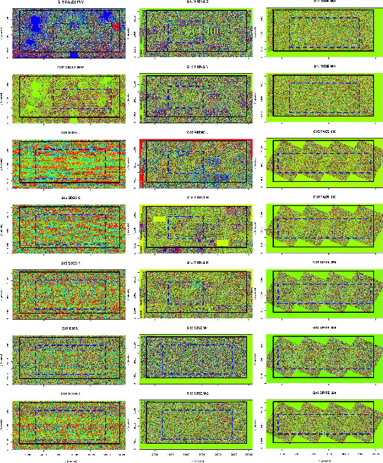
Figure 29: Background uniformity and coverage in the G15 region for GALEX, SDSS, VIKING, WISE and Herschel data.

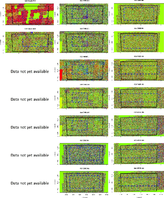
Figure 30: Background uniformity and coverage in the G23 region for GALEX, VIKING, WISE and Herschel data.

Appendix A GAMA PDR coverage

Figs. 27 to 30 shows the GAMA PDR coverage in each of the 21 bands, all data is available for download via: http://gama-psi.icrar.org/