DQM: Decentralized Quadratically Approximated Alternating Direction Method of Multipliers

Abstract

This paper considers decentralized consensus optimization problems where nodes of a network have access to different summands of a global objective function. Nodes cooperate to minimize the global objective by exchanging information with neighbors only. A decentralized version of the alternating directions method of multipliers (DADMM) is a common method for solving this category of problems. DADMM exhibits linear convergence rate to the optimal objective but its implementation requires solving a convex optimization problem at each iteration. This can be computationally costly and may result in large overall convergence times. The decentralized quadratically approximated ADMM algorithm (DQM), which minimizes a quadratic approximation of the objective function that DADMM minimizes at each iteration, is proposed here. The consequent reduction in computational time is shown to have minimal effect on convergence properties. Convergence still proceeds at a linear rate with a guaranteed constant that is asymptotically equivalent to the DADMM linear convergence rate constant. Numerical results demonstrate advantages of DQM relative to DADMM and other alternatives in a logistic regression problem.

I Introduction

Decentralized algorithms are used to solve optimization problems where components of the objective are available at different nodes of a network. Nodes access their local cost functions only but try to minimize the aggregate cost by exchanging information with their neighbors. Specifically, consider a variable ${\tilde{\mathbf{x}}}\in{\mathbb{R}}^{p}$ and a connected network containing $n$ nodes each of which has access to a local cost function $f_{i}:{\mathbb{R}}^{p}\to{\mathbb{R}}$. The nodes’ goal is to find the optimal argument of the global cost function $\sum_{i=1}^{n}f_{i}({\tilde{\mathbf{x}}})$,

$${\tilde{\mathbf{x}}}^{*}\ =\ \operatornamewithlimits{argmin}_{{\tilde{\mathbf{x}}}}\sum_{i=1}^{n}f_{i}({\tilde{\mathbf{x}}}).$$ (1)

Problems of this form arise in, e.g., decentralized control [2, 3, 4], wireless communication [5, 6], sensor networks [7, 8, 9], and large scale machine learning [10, 11, 12]. In this paper we assume that the local costs $f_{i}$ are twice differentiable and strongly convex.

There are different algorithms to solve (1) in a decentralized manner which can be divided into two major categories. The ones that operate in the primal domain and the ones that operate in the dual domain. Among primal domain algorithms, decentralized (sub)gradient descent (DGD) methods are well studied [13, 14, 15]. They can be interpreted as either a mix of local gradient descent steps with successive averaging or as a penalized version of (1) with a penalty term that encourages agreement between adjacent nodes. This latter interpretation has been exploited to develop the network Newton (NN) methods that attempt to approximate the Newton step of this penalized objective in a distributed manner [16, 17]. The methods that operate in the dual domain consider a constraint that enforces equality between nodes’ variables. They then ascend on the dual function to find optimal Lagrange multipliers with the solution of (1) obtained as a byproduct [7, 18, 19, 20]. Among dual descent methods, decentralized implementation of the alternating directions method of multipliers (ADMM), known as DADMM, is proven to be very efficient with respect to convergence time [7, 18, 19].

A fundamental distinction between primal methods such as DGD and NN and dual domain methods such as DADMM is that the former compute local gradients and Hessians at each iteration while the latter minimize local pieces of the Lagrangian at each step – this is necessary since the gradient of the dual function is determined by Lagrangian minimizers. Thus, iterations in dual domain methods are, in general, more costly because they require solution of a convex optimization problem. However, dual methods also converge in a smaller number of iterations because they compute approximations to ${\tilde{\mathbf{x}}}^{*}$ instead of descending towards ${\tilde{\mathbf{x}}}^{*}$. Having complementary advantages, the choice between primal and dual methods depends on the relative cost of computation and communication for specific problems and platforms. Alternatively, one can think of developing methods that combine the advantages of ascending in the dual domain without requiring solution of an optimization problem at each iteration. This can be accomplished by the decentralized linearized ADMM (DLM) algorithm [21, 22], which replaces the minimization of a convex objective required by ADMM with the minimization of a first order linear approximation of the objective function. This yields per-iteration problems that can be solved with a computational cost akin to the computation of a gradient and a method with convergence properties closer to DADMM than DGD.

If a first order approximation of the objective is useful, a second order approximation should decrease convergence times further. The decentralized quadratically approximated ADMM (DQM) algorithm that we propose here minimizes a quadratic approximation of the Lagrangian minimization of each ADMM step. This quadratic approximation requires computation of local Hessians but results in an algorithm with convergence properties that are: (i) better than the convergence properties of DLM; (ii) asymptotically identical to the convergence behavior of DADMM. The technical contribution of this paper is to prove that (i) and (ii) are true from both analytical and practical perspectives.

We begin the paper by discussing solution of (1) with DADMM and its linearized version DLM (Section II). Both of these algorithms perform updates on dual and primal auxiliary variables that are identical and computationally simple. They differ in the manner in which principal primary variables are updated. DADMM solves a convex optimization problem and DLM solves a regularized linear approximation. We follow with an explanation of DQM that differs from DADMM and DLM in that it minimizes a quadratic approximation of the convex problem that DADMM solves exactly and DLM approximates linearly (Section III). We also explain how DQM can be implemented in a distributed manner (Proposition 1 and Algorithm 1). Convergence properties of DQM are then analyzed (Section IV) where linear convergence is established (Theorem 1 and Corollary 1). Key in the analysis is the error incurred when approximating the exact minimization of DADMM with the quadratic approximation of DQM. This error is shown to decrease as iterations progress (Proposition 2) faster than the rate that the error of DLM approaches zero (Proposition 3). This results in DQM having a guaranteed convergence constant strictly smaller than the DLM constant that approaches the guaranteed constant of DADMM for large iteration index (Section IV-A). We corroborate analytical results with numerical evaluations in a logistic regression problem (Section V). We show that DQM does outperform DLM and show that convergence paths of DQM and DADMM are almost identical (Section V-A). Overall computational cost of DQM is shown to be smaller, as expected.

Notation. Vectors are written as ${\mathbf{x}}\in{\mathbb{R}}^{n}$ and matrices as ${\mathbf{A}}\in{\mathbb{R}}^{n\times n}$. Given $n$ vectors ${\mathbf{x}}_{i}$, the vector ${\mathbf{x}}=[{\mathbf{x}}_{1};\ldots;{\mathbf{x}}_{n}]$ represents a stacking of the elements of each individual ${\mathbf{x}}_{i}$. We use $\|{\mathbf{x}}\|$ to denote the Euclidean norm of vector ${\mathbf{x}}$ and $\|{\mathbf{A}}\|$ to denote the Euclidean norm of matrix ${\mathbf{A}}$. The gradient of a function $f$ at point ${\mathbf{x}}$ is denoted as $\nabla f({\mathbf{x}})$ and the Hessian is denoted as $\nabla^{2}f({\mathbf{x}})$. We use $\sigma({\mathbf{B}})$ to denote the singular values of matrix ${\mathbf{B}}$ and $\lambda({\mathbf{A}})$ to denote the eigenvalues of matrix ${\mathbf{A}}$.

II Distributed Alternating Directions Method of Multipliers

Consider a connected network with $n$ nodes and $m$ edges where the set of nodes is $\mathcal{V}=\{1,\dots,n\}$ and the set of ordered edges $\mathcal{E}$ contains pairs $(i,j)$ indicating that $i$ can communicate to $j$. We restrict attention to symmetric networks in which $(i,j)\in\mathcal{E}$ if and only if $(j,i)\in\mathcal{E}$ and define node $i$’s neighborhood as the set $\mathcal{N}_{i}=\{j\mid(i,j)\in\mathcal{E}\}$. In problem (1) agent $i$ has access to the local objective function $f_{i}({\tilde{\mathbf{x}}})$ and agents cooperate to minimize the global cost $\sum_{i=1}^{n}f_{i}({\tilde{\mathbf{x}}})$. This specification is more naturally formulated by defining variables ${\mathbf{x}}_{i}$ representing the local copies of the variable ${\tilde{\mathbf{x}}}$. We also define the auxiliary variables ${\mathbf{z}}_{ij}$ associated with edge $(i,j)\in\mathcal{E}$ and rewrite (1) as

$$\{{\mathbf{x}}_{i}^{*}\}_{i=1}^{n}:=\ \operatornamewithlimits{argmin}_{{\mathbf{x}}} \ \sum_{i=1}^{n}\ f_{i}({\mathbf{x}}_{i}),$$ (2)

$$\operatornamewithlimits{s.t.} \ {\mathbf{x}}_{i}={\mathbf{z}}_{ij},\ {\mathbf{x}}_{j}={\mathbf{z}}_{ij},\ \text{for all\ }(i,j)\in{\mathcal{E}}.$$

The constraints ${\mathbf{x}}_{i}={\mathbf{z}}_{ij}$ and ${\mathbf{x}}_{j}={\mathbf{z}}_{ij}$ enforce that the variable ${\mathbf{x}}_{i}$ of each node $i$ is equal to the variables ${\mathbf{x}}_{j}$ of its neighbors $j\in{\mathcal{N}}_{i}$. This condition in association with network connectivity implies that a set of variables $\{{\mathbf{x}}_{1},\dots,{\mathbf{x}}_{n}\}$ is feasible for problem (2) if and only if all the variables ${\mathbf{x}}_{i}$ are equal to each other, i.e., if ${\mathbf{x}}_{1}=\dots={\mathbf{x}}_{n}$. Therefore, problems (1) and (2) are equivalent in the sense that for all $i$ and $j$ the optimal arguments of (2) satisfy ${\mathbf{x}}_{i}^{*}={\tilde{\mathbf{x}}}^{*}$ and ${\mathbf{z}}_{ij}={\tilde{\mathbf{x}}}^{*}$, where ${\tilde{\mathbf{x}}}^{*}$ is the optimal argument of (1).

To write problem (2) in a matrix form, define ${\mathbf{A}}_{s}\in{\mathbb{R}}^{mp\times np}$ as the block source matrix which contains $m\times n$ square blocks $({\mathbf{A}}_{s})_{e,i}\in{\mathbb{R}}^{p\times p}$. The block $({\mathbf{A}}_{s})_{e,i}$ is not identically null if and only if the edge $e$ corresponds to $e=(i,j)\in{\mathcal{E}}$ in which case $({\mathbf{A}}_{s})_{e,i}={\mathbf{I}}_{p}$. Likewise, the block destination matrix ${\mathbf{A}}_{d}\in{\mathbb{R}}^{mp\times np}$ contains $m\times n$ square blocks $({\mathbf{A}}_{d})_{e,i}\in{\mathbb{R}}^{p\times p}$. The square block $({\mathbf{A}}_{d})_{e,i}={\mathbf{I}}_{p}$ when $e$ corresponds to $e=(j,i)\in{\mathcal{E}}$ and is null otherwise. Further define ${\mathbf{x}}:=[{\mathbf{x}}_{1};\dots;{\mathbf{x}}_{n}]\in{\mathbb{R}}^{np}$ as a vector concatenating all local variables ${\mathbf{x}}_{i}$, the vector ${\mathbf{z}}:=[{\mathbf{z}}_{1};\dots;{\mathbf{z}}_{m}]\in{\mathbb{R}}^{mp}$ concatenating all auxiliary variables ${\mathbf{z}}_{e}={\mathbf{z}}_{ij}$, and the aggregate function $f:{\mathbb{R}}^{np}\to{\mathbb{R}}$ as $f({\mathbf{x}}):=\sum_{i=1}^{n}f_{i}({\mathbf{x}}_{i})$. We can then rewrite (2) as

$${\mathbf{x}}^{*}:=\operatornamewithlimits{argmin}_{{\mathbf{x}}}f({\mathbf{x}}),\quad\operatornamewithlimits{s.t.}\ {\mathbf{A}}_{s}{\mathbf{x}}-{\mathbf{z}}={\mathbf{0}},\ {\mathbf{A}}_{d}{\mathbf{x}}-{\mathbf{z}}={\mathbf{0}}.$$ (3)

Define now the matrix ${\mathbf{A}}=[{\mathbf{A}}_{s};{\mathbf{A}}_{d}]\in{\mathbb{R}}^{2mp\times np}$ which stacks the source and destination matrices, and the matrix ${\mathbf{B}}=[-{\mathbf{I}}_{mp};-{\mathbf{I}}_{mp}]\in{\mathbb{R}}^{2mp\times mp}$ which stacks two negative identity matrices of size $mp$ to rewrite (3) as

$${\mathbf{x}}^{*}:=\operatornamewithlimits{argmin}_{{\mathbf{x}}}f({\mathbf{x}}),\quad\operatornamewithlimits{s.t.}\ {\mathbf{A}}{\mathbf{x}}+{\mathbf{B}}{\mathbf{z}}={\mathbf{0}}.$$ (4)

DADMM is the application of ADMM to solve (4). To develop this algorithm introduce Lagrange multipliers $\boldsymbol{\alpha}_{e}=\boldsymbol{\alpha}_{ij}$ and $\boldsymbol{\beta}_{e}=\boldsymbol{\beta}_{ij}$ associated with the constraints ${\mathbf{x}}_{i}={\mathbf{z}}_{ij}$ and ${\mathbf{x}}_{j}={\mathbf{z}}_{ij}$ in (2), respectively. Define $\boldsymbol{\alpha}:=[\boldsymbol{\alpha}_{1};\dots;\boldsymbol{\alpha}_{m}]$ as the concatenation of the multipliers $\boldsymbol{\alpha}_{e}$ which yields the multiplier of the constraint ${\mathbf{A}}_{s}{\mathbf{x}}-{\mathbf{z}}={\mathbf{0}}$ in (3). Likewise, the corresponding Lagrange multiplier of the constraint ${\mathbf{A}}_{d}{\mathbf{x}}-{\mathbf{z}}={\mathbf{0}}$ in (3) can be obtained by stacking the multipliers $\boldsymbol{\beta}_{e}$ to define $\boldsymbol{\beta}:=[\boldsymbol{\beta}_{1};\dots;\boldsymbol{\beta}_{m}]$. Grouping $\boldsymbol{\alpha}$ and $\boldsymbol{\beta}$ into $\boldsymbol{\lambda}:=[\boldsymbol{\alpha};\boldsymbol{\beta}]\in{\mathbb{R}}^{2mp}$ leads to the Lagrange multiplier $\boldsymbol{\lambda}$ associated with the constraint ${\mathbf{A}}{\mathbf{x}}+{\mathbf{B}}{\mathbf{z}}={\mathbf{0}}$ in (4). Using these definitions and introducing a positive constant $c>0$ we write the augmented Lagrangian of (4) as

$${\mathcal{L}}({\mathbf{x}},{\mathbf{z}},\boldsymbol{\lambda}):=f({\mathbf{x}})+\boldsymbol{\lambda}^{T}\left({\mathbf{A}}{\mathbf{x}}+{\mathbf{B}}{\mathbf{z}}\right)+\frac{c}{2}\left\|{\mathbf{A}}{\mathbf{x}}+{\mathbf{B}}{\mathbf{z}}\right\|^{2}.$$ (5)

The idea of ADMM is to minimize the Lagrangian ${\mathcal{L}}({\mathbf{x}},{\mathbf{z}},\boldsymbol{\lambda})$ with respect to ${\mathbf{x}}$, follow by minimizing the updated Lagrangian with respect to ${\mathbf{z}}$, and finish each iteration with an update of the multiplier $\boldsymbol{\lambda}$ using dual ascent. To be more precise, consider the time index $k\in{\mathbb{N}}$ and define ${\mathbf{x}}_{k}$, ${\mathbf{z}}_{k}$, and $\boldsymbol{\lambda}_{k}$ as the iterates at step $k$. At this step, the augmented Lagrangian is minimized with respect to ${\mathbf{x}}$ to obtain the iterate

$${\mathbf{x}}_{k+1}=\operatornamewithlimits{argmin}_{{\mathbf{x}}}f({\mathbf{x}})+\boldsymbol{\lambda}_{k}^{T}\left({\mathbf{A}}{\mathbf{x}}+{\mathbf{B}}{\mathbf{z}}_{k}\right)+\frac{c}{2}\left\|{\mathbf{A}}{\mathbf{x}}+{\mathbf{B}}{\mathbf{z}}_{k}\right\|^{2}.$$ (6)

Then, the augmented Lagrangian is minimized with respect to the auxiliary variable ${\mathbf{z}}$ using the updated variable ${\mathbf{x}}_{k+1}$ to obtain

$${\mathbf{z}}_{k+1}=\operatornamewithlimits{argmin}_{{\mathbf{z}}} \ f({\mathbf{x}}_{k+1})$$ (7)

$$+\boldsymbol{\lambda}_{k}^{T}\left({\mathbf{A}}{\mathbf{x}}_{k+1}+{\mathbf{B}}{\mathbf{z}}\right)+\frac{c}{2}\left\|{\mathbf{A}}{\mathbf{x}}_{k+1}+{\mathbf{B}}{\mathbf{z}}\right\|^{2}.$$

After updating the variables ${\mathbf{x}}$ and ${\mathbf{z}}$, the Lagrange multiplier $\boldsymbol{\lambda}_{k}$ is updated through the dual ascent iteration

$$\boldsymbol{\lambda}_{k+1}=\boldsymbol{\lambda}_{k}+c\left({\mathbf{A}}{\mathbf{x}}_{k+1}+{\mathbf{B}}{\mathbf{z}}_{k+1}\right).$$ (8)

The DADMM algorithm is obtained by observing that the structure of the matrices ${\mathbf{A}}$ and ${\mathbf{B}}$ is such that (6)-(8) can be implemented in a distributed manner [7, 18, 19].

The updates for the auxiliary variable ${\mathbf{z}}$ and the Lagrange multiplier $\boldsymbol{\lambda}$ are not costly in terms of computation time. However, updating the primal variable ${\mathbf{x}}$ can be expensive as it entails the solution of an optimization problem [cf. (6)]. The DLM algorithm avoids this cost with an inexact update of the primal variable iterate ${\mathbf{x}}_{k+1}$. This inexact update relies on approximating the aggregate function value $f({\mathbf{x}}_{k+1})$ in (6) through a regularized linearization of the aggregate function $f$ in a neighborhood of the current variable ${\mathbf{x}}_{k}$. This regularized approximation takes the form $f({\mathbf{x}})\approx f({\mathbf{x}}_{k})+\nabla f({\mathbf{x}}_{k})^{T}({\mathbf{x}}-{\mathbf{x}}_{k})+(\rho/2)\|{\mathbf{x}}-{\mathbf{x}}_{k}\|^{2}$ for a given positive constant $\rho>0$. Consequently, the update formula for the primal variable ${\mathbf{x}}$ in DLM replaces the DADMM exact minimization in (6) by the minimization of the quadratic form

$${\mathbf{x}}_{k+1}=\operatornamewithlimits{argmin}_{{\mathbf{x}}}\ f({\mathbf{x}}_{k})+\nabla f({\mathbf{x}}_{k})^{T}({\mathbf{x}}-{\mathbf{x}}_{k})+\frac{\rho}{2}\|{\mathbf{x}}-{\mathbf{x}}_{k}\|^{2}$$

$$\quad+\boldsymbol{\lambda}_{k}^{T}\left({\mathbf{A}}{\mathbf{x}}+{\mathbf{B}}{\mathbf{z}}_{k}\right)+\frac{c}{2}\left\|{\mathbf{A}}{\mathbf{x}}+{\mathbf{B}}{\mathbf{z}}_{k}\right\|^{2}.$$ (9)

The first order optimality condition for (II) implies that the updated variable ${\mathbf{x}}_{k+1}$ satisfies

$$\nabla f({\mathbf{x}}_{k})+\rho({\mathbf{x}}_{k+1}-{\mathbf{x}}_{k})+{\mathbf{A}}^{T}\boldsymbol{\lambda}_{k}+c{\mathbf{A}}^{T}\left({\mathbf{A}}{\mathbf{x}}_{k+1}+{\mathbf{B}}{\mathbf{z}}_{k}\right)={\mathbf{0}}.$$ (10)

According to (10), the updated variable ${\mathbf{x}}_{k+1}$ can be computed by inverting the positive definite matrix $\rho{\mathbf{I}}+c{\mathbf{A}}^{T}{\mathbf{A}}$. This update can also be implemented in a distributed manner.

The sequence of variables ${\mathbf{x}}_{k}$ generated by DLM converges linearly to the optimal argument ${\mathbf{x}}^{*}$ [21]. Although this is the same rate of DADMM, linear convergence constant of DLM is smaller than the one for DADMM (see Section IV-A), and can be much smaller depending on the condition number of the local functions $f_{i}$ (see Section V-A). To close the gap between these constants we can use a second order approximation of (6). This is the idea of DQM that we introduce in the following section.

III DQM: Decentralized Quadratically Approximated ADMM

DQM uses a local quadratic approximation of the primal function $f({\mathbf{x}})$ around the current iterate ${\mathbf{x}}_{k}$. If we let ${\mathbf{H}}_{k}:=\nabla^{2}f({\mathbf{x}}_{k})$ denote the primal function Hessian evaluated at ${\mathbf{x}}_{k}$ the quadratic approximation of $f$ at ${\mathbf{x}}_{k}$ is $f({\mathbf{x}})\approx f({\mathbf{x}}_{k})+\nabla f({\mathbf{x}}_{k})^{T}({\mathbf{x}}-{\mathbf{x}}_{k})+(1/2)({\mathbf{x}}-{\mathbf{x}}_{k})^{T}{\mathbf{H}}_{k}({\mathbf{x}}-{\mathbf{x}}_{k})$. Using this approximation in (6) yields the DQM update that we therefore define as

$${\mathbf{x}}_{k+1}:=\operatornamewithlimits{argmin}_{{\mathbf{x}}}f( {\mathbf{x}}_{k})+\nabla f({\mathbf{x}}_{k})^{T}({\mathbf{x}}-{\mathbf{x}}_{k})$$ (11)

$$+\frac{1}{2}({\mathbf{x}}-{\mathbf{x}}_{k})^{T}{\mathbf{H}}_{k}({\mathbf{x}}-{\mathbf{x}}_{k})$$

$$+\boldsymbol{\lambda}_{k}^{T}\left({\mathbf{A}}{\mathbf{x}}+{\mathbf{B}}{\mathbf{z}}_{k}\right)+\frac{c}{2}\left\|{\mathbf{A}}{\mathbf{x}}+{\mathbf{B}}{\mathbf{z}}_{k}\right\|^{2}.$$

Comparison of (II) and (11) shows that in DLM the quadratic term $(\rho/2)\|{\mathbf{x}}_{k+1}-{\mathbf{x}}_{k}\|^{2}$ is added to the first-order approximation of the primal objective function, while in DQM the second order approximation of the primal objective function is used to reach a more accurate approximation for $f({\mathbf{x}})$. Since (11) is a quadratic program, the first order optimality condition yields a system of linear equations that can be solved to find ${\mathbf{x}}_{k+1}$,

$$\nabla f({\mathbf{x}}_{k})+{\mathbf{H}}_{k}({\mathbf{x}}_{k+1}\!-\!{\mathbf{x}}_{k})+{\mathbf{A}}^{T}\!\boldsymbol{\lambda}_{k}+c{\mathbf{A}}^{T}\!\left({\mathbf{A}}{\mathbf{x}}_{k+1}+{\mathbf{B}}{\mathbf{z}}_{k}\right)={\mathbf{0}}.$$ (12)

This update can be solved by inverting the matrix ${\mathbf{H}}_{k}+c{\mathbf{A}}^{T}{\mathbf{A}}$ which is invertible if, as we are assuming, $f({\mathbf{x}})$ is strongly convex.

The DADMM updates in (7) and (8) are used verbatim in DQM, which is therefore defined by recursive application of (12), (7), and (8). It is customary to consider the first order optimality conditions of (7) and to reorder terms in (8) to rewrite the respective updates as

$${\mathbf{B}}^{T}\boldsymbol{\lambda}_{k}+c{\mathbf{B}}^{T}\left({\mathbf{A}}{\mathbf{x}}_{k+1}+{\mathbf{B}}{\mathbf{z}}_{k+1}\right) ={\mathbf{0}},$$

$$\boldsymbol{\lambda}_{k+1}-\boldsymbol{\lambda}_{k}-c\left({\mathbf{A}}{\mathbf{x}}_{k+1}+{\mathbf{B}}{\mathbf{z}}_{k+1}\right) ={\mathbf{0}}.$$ (13)

DQM is then equivalently defined by recursive solution of the system of linear equations in (12) and (III). This system, as is the case of DADMM and DLM, can be reworked into a simpler form that reduces communication cost. To derive this simpler form we assume a specific structure for the initial vectors $\boldsymbol{\lambda}_{0}=[\boldsymbol{\alpha}_{0};\boldsymbol{\beta}_{0}]$, ${\mathbf{x}}_{0}$, and ${\mathbf{z}}_{0}$ as introduced in the following assumption.

Assumption 1

Define the oriented incidence matrix as ${\mathbf{E}}_{o}:={\mathbf{A}}_{s}-{\mathbf{A}}_{d}$ and the unoriented incidence matrix as ${\mathbf{E}}_{u}:={\mathbf{A}}_{s}+{\mathbf{A}}_{d}$. The initial Lagrange multipliers $\boldsymbol{\alpha}_{0}$ and $\boldsymbol{\beta}_{0}$, and the initial variables ${\mathbf{x}}_{0}$ and ${\mathbf{z}}_{0}$ are chosen such that:

1. The multipliers are opposites of each other, $\boldsymbol{\alpha}_{0}=-\boldsymbol{\beta}_{0}$.

2. The initial primal variables satisfy ${\mathbf{E}}_{u}{\mathbf{x}}_{0}=2{\mathbf{z}}_{0}$.

3. The initial multiplier $\boldsymbol{\alpha}_{0}$ lies in the column space of ${\mathbf{E}}_{o}$.

Assumption 1 is minimally restrictive. The only non-elementary condition is (c) but that can be satisfied by $\boldsymbol{\alpha}_{0}={\mathbf{0}}$. Nulling all other variables, i.e., making $\boldsymbol{\beta}_{0}={\mathbf{0}}$, ${\mathbf{x}}_{0}={\mathbf{0}}$, and ${\mathbf{z}}_{0}={\mathbf{0}}$ is a trivial choice to comply with conditions (a) and (b) as well. An important consequence of the initialization choice in (1) is that if the conditions in Assumption 1 are true at time $k=0$ they stay true for all subsequent iterations $k>0$ as we state next.

Lemma 1

Consider the DQM algorithm as defined by (12)-(III). If Assumption 1 holds, then for all $k\geq 0$ the Lagrange multipliers $\boldsymbol{\alpha}_{k}$ and $\boldsymbol{\beta}_{k}$, and the variables ${\mathbf{x}}_{k}$ and ${\mathbf{z}}_{k}$ satisfy:

1. The multipliers are opposites of each other, $\boldsymbol{\alpha}_{k}=-\boldsymbol{\beta}_{k}$.

2. The primal variables satisfy ${\mathbf{E}}_{u}{\mathbf{x}}_{k}=2{\mathbf{z}}_{k}$.

3. The multiplier $\boldsymbol{\alpha}_{k}$ lies in the column space of ${\mathbf{E}}_{o}$.

Proof : See Appendix A. $\blacksquare$

The validity of (c) in Lemma 1 is important for the convergence analysis of Section IV. The validity of (a) and (b) means that maintaining multipliers $\boldsymbol{\alpha}_{k}$ and $\boldsymbol{\beta}_{k}$ is redundant because they are opposites and that maintaining variables ${\mathbf{z}}_{k}$ is also redundant because they can be computed as ${\mathbf{z}}_{k}={\mathbf{E}}_{u}{\mathbf{x}}_{k}/2$. It is then possible to replace (12)-(III) by a simpler system of linear equations as we explain in the following proposition.

Proposition 1

Consider the DQM algorithm as defined by (12)-(III) and define the sequence $\boldsymbol{\phi}_{k}:={\mathbf{E}}_{o}^{T}\boldsymbol{\alpha}_{k}$. Further define the unoriented Laplacian as ${\mathbf{L}}_{u}:=(1/2){\mathbf{E}}_{u}^{T}{\mathbf{E}}_{u}$, the oriented Laplacian as ${\mathbf{L}}_{o}=(1/2){\mathbf{E}}_{o}^{T}{\mathbf{E}}_{o}$, and the degree matrix as ${\mathbf{D}}:=({\mathbf{L}}_{u}+{\mathbf{L}}_{o})/2$. If Assumption 1 holds true, the DQM iterates ${\mathbf{x}}_{k}$ can be generated as

$${\mathbf{x}}_{k+1} =(2c{\mathbf{D}}+{\mathbf{H}}_{k})^{-1}\left[(c{\mathbf{L}}_{u}+{\mathbf{H}}_{k}){\mathbf{x}}_{k}-\nabla f({\mathbf{x}}_{k})-\boldsymbol{\phi}_{k}\right],$$

$$\boldsymbol{\phi}_{k+1} =\boldsymbol{\phi}_{k}+c{\mathbf{L}}_{o}{\mathbf{x}}_{k+1}.$$ (14)

Proof : See Appendix B. $\blacksquare$

Proposition 1 states that by introducing the sequence of variables $\boldsymbol{\phi}_{k}$, the DQM primal iterates ${\mathbf{x}}_{k}$ can be computed through the recursive expressions in (1). These recursions are simpler than (12)-(III) because they eliminate the auxiliary variables ${\mathbf{z}}_{k}$ and reduce the dimensionality of $\boldsymbol{\lambda}_{k}$ – twice the number of edges – to that of $\boldsymbol{\phi}_{k}$ – the number of nodes. Further observe that if (1) is used for implementation we don’t have to make sure that the conditions of Assumption 1 are satisfied. We just need to pick $\boldsymbol{\phi}_{0}:={\mathbf{E}}_{o}^{T}\boldsymbol{\alpha}_{0}$ for some $\boldsymbol{\alpha}_{0}$ in the column space of ${\mathbf{E}}_{0}$ – which is not difficult, we can use, e.g., $\boldsymbol{\phi}_{0}={\mathbf{0}}$. The role of Assumption 1 is to state conditions for which the expressions in (12)-(III) are an equivalent representation of (1) that we use for convergence analyses.

The structure of the primal objective function Hessian ${\mathbf{H}}_{k}$, the degree matrix ${\mathbf{D}}$, and the oriented and unoriented Laplacians ${\mathbf{L}}_{o}$ and ${\mathbf{L}}_{u}$ make distributed implementation of (1) possible. Indeed, the matrix $2c{\mathbf{D}}+{\mathbf{H}}_{k}$ is block diagonal and its $i$-th diagonal block is given by $2cd_{i}{\mathbf{I}}+\nabla^{2}f_{i}({\mathbf{x}}_{i})$ which is locally available for node $i$. Likewise, the inverse matrix $(2c{\mathbf{D}}+{\mathbf{H}}_{k})^{-1}$ is block diagonal and locally computable since the $i$-th diagonal block is $(2cd_{i}{\mathbf{I}}+\nabla^{2}f_{i}({\mathbf{x}}_{i}))^{-1}$. Computations of the products ${\mathbf{L}}_{u}{\mathbf{x}}_{k}$ and ${\mathbf{L}}_{o}{\mathbf{x}}_{k+1}$ can be implemented in a decentralized manner as well, since the Laplacian matrices ${\mathbf{L}}_{u}$ and ${\mathbf{L}}_{o}$ are block neighbor sparse in the sense that the ${(i,j)}$-th block is not null if and only if nodes $i$ and $j$ are neighbors or $j=i$. Therefore, nodes can compute their local parts for the products ${\mathbf{L}}_{u}{\mathbf{x}}_{k}$ and ${\mathbf{L}}_{o}{\mathbf{x}}_{k+1}$ by exchanging information with their neighbors. By defining components of the vector $\boldsymbol{\phi}_{k}$ as $\boldsymbol{\phi}_{k}:=[\boldsymbol{\phi}_{1,k},\dots,\boldsymbol{\phi}_{n,k}]$, the update formula in (1) for the individual agents can then be written block-wise as

$${\mathbf{x}}_{i,k+1}=\ \left(2cd_{i}{\mathbf{I}}+\nabla^{2}f_{i}({\mathbf{x}}_{i,k})\right)^{-1}\Big{[}cd_{i}{\mathbf{x}}_{i,k}+c\sum_{j\in{\mathcal{N}}_{i}}{\mathbf{x}}_{j,k}$$

$$\qquad+\nabla^{2}f_{i}({\mathbf{x}}_{i,k}){\mathbf{x}}_{i,k}-\nabla f_{i}({\mathbf{x}}_{i,k})-\boldsymbol{\phi}_{i,k}\Big{]},$$ (15)

where ${\mathbf{x}}_{i,k}$ corresponds to the iterate of node $i$ at step $k$. Notice that the defintion ${\mathbf{L}}_{u}:=(1/2){\mathbf{E}}_{u}^{T}{\mathbf{E}}_{u}=(1/2)({\mathbf{A}}_{s}+{\mathbf{A}}_{d})^{T}({\mathbf{A}}_{s}+{\mathbf{A}}_{d})$ is used to simplify the $i$-th component of $c{\mathbf{L}}_{u}{\mathbf{x}}_{k}$ as $c\sum_{j\in{\mathcal{N}}_{i}}({\mathbf{x}}_{i,k}+{\mathbf{x}}_{j,k})$ which is equivalent to $cd_{i}{\mathbf{x}}_{i,k}+c\sum_{j\in{\mathcal{N}}_{i}}{\mathbf{x}}_{j,k}$. Further, using the definition ${\mathbf{L}}_{o}=(1/2){\mathbf{E}}_{o}^{T}{\mathbf{E}}_{o}=(1/2)({\mathbf{A}}_{s}-{\mathbf{A}}_{d})^{T}({\mathbf{A}}_{s}-{\mathbf{A}}_{d})$, the $i$-th component of the product $c{\mathbf{L}}_{o}{\mathbf{x}}_{k+1}$ in (16) can be simplified as $c\sum_{j\in{\mathcal{N}}_{i}}({\mathbf{x}}_{i,k}-{\mathbf{x}}_{j,k})$. Therefore, the second update formula in (1) can be locally implemented at each node $i$ as

$$\boldsymbol{\phi}_{i,k+1}=\boldsymbol{\phi}_{i,k}+c\sum_{j\in{\mathcal{N}}_{i}}\left({\mathbf{x}}_{i,k+1}-{\mathbf{x}}_{j,k+1}\right).$$ (16)

The proposed DQM method is summarized in Algorithm 1. The initial value for the local iterate ${\mathbf{x}}_{i,0}$ can be any arbitrary vector in ${\mathbb{R}}^{p}$. The initial vector $\boldsymbol{\phi}_{i,0}$ should be in column space of ${\mathbf{E}}_{o}^{T}$. To guarantee satisfaction of this condition, the initial vector is set as $\boldsymbol{\phi}_{i,0}={\mathbf{0}}$. At each iteration $k$, updates of the primal and dual variables in (III) and (16) are computed in Steps 2 and 4, respectively. Nodes exchange their local variables ${\mathbf{x}}_{i,k}$ with their neighbors $j\in{\mathcal{N}}_{i}$ in Step 3, since this information is required for the updates in Steps 2 and 4.

Algorithm 1 DQM method at node $i$

0:  Initial local iterates ${\mathbf{x}}_{i,0}$ and $\boldsymbol{\phi}_{0}$.

1:  for $k=0,1,2,\ldots$ do

2:     Update the local iterate ${\mathbf{x}}_{i,k+1}$ as

$${\mathbf{x}}_{i,k+1}=\ \left(2cd_{i}{\mathbf{I}}+\nabla^{2}f_{i}({\mathbf{x}}_{i,k})\right)^{-1}\bigg{[}cd_{i}{\mathbf{x}}_{i,k}+c\sum_{j\in{\mathcal{N}}_{i}}{\mathbf{x}}_{j,k}$$

$$\qquad\qquad+\nabla^{2}f_{i}({\mathbf{x}}_{i,k}){\mathbf{x}}_{i,k}-\nabla f_{i}({\mathbf{x}}_{i,k})-\boldsymbol{\phi}_{i,k}\bigg{]}.$$

3:     Exchange iterates ${\mathbf{x}}_{i,k+1}$ with neighbors $\displaystyle{j\in\mathcal{N}_{i}}$.

4:     Update local dual variable $\boldsymbol{\phi}_{k+1}$ as $\displaystyle{\qquad\boldsymbol{\phi}_{i,k+1}=\boldsymbol{\phi}_{i,k}+c\sum_{j\in{\mathcal{N}}_{i}}\left({\mathbf{x}}_{i,k+1}-{\mathbf{x}}_{j,k+1}\right).}$

5:  end for

DADMM, DQM, and DLM occupy different points in a tradeoff curve of computational cost per iteration and number of iterations needed to achieve convergence. The computational cost of each DADMM iteration is large in general because it requires solution of the optimization problem in (6). The cost of DLM iterations is minimal because the solution of (10) can be reduced to the inversion of a block diagonal matrix; see [22]. The cost of DQM iterations is larger than the cost of DLM iterations because they require evaluation of local Hessians as well as inversion of the matrices $2cd_{i}{\mathbf{I}}+\nabla^{2}f_{i}({\mathbf{x}}_{i,k})$ to implement (III). But the cost is smaller than the cost of DADMM iterations except in cases in which solving (6) is easy. In terms of the number of iterations required until convergence, DADMM requires the least and DLM the most. The foremost technical conclusions of the convergence analysis presented in the following section are: (i) convergence of DQM is strictly faster than convergence of DLM; (ii) asymptotically in the number of iterations, the per iteration improvements of DADMM and DQM are identical. It follows from these observations that DQM achieves target optimality in a number of iterations similar to DADMM but with iterations that are computationally cheaper.

IV Convergence Analysis

In this section we show that the sequence of iterates ${\mathbf{x}}_{k}$ generated by DQM converges linearly to the optimal argument ${\mathbf{x}}^{*}=[{\tilde{\mathbf{x}}}^{*};\dots;{\tilde{\mathbf{x}}}^{*}]$. As a byproduct of this analysis we also obtain a comparison between the linear convergence constants of DLM, DQM, and DADMM. To derive these results we make the following assumptions.

Assumption 2

The network is such that any singular value of the unoriented incidence matrix ${\mathbf{E}}_{u}$, defined as $\sigma({\mathbf{E}}_{u})$, satisfies $0<\gamma_{u}\leq\sigma({\mathbf{E}}_{u})\leq\Gamma_{u}$ where $\gamma_{u}$ and $\Gamma_{u}$ are constants; the smallest non-zero singular value of the oriented incidence matrix ${\mathbf{E}}_{o}$ is $\gamma_{o}>0$.

Assumption 3

The local objective functions $f_{i}({\mathbf{x}})$ are twice differentiable and the eigenvalues of their local Hessians $\nabla^{2}f_{i}({\mathbf{x}})$ are bounded within positive constants $m$ and $M$ where $0<m\leq M<\infty$ so that for all ${\mathbf{x}}\in{\mathbb{R}}^{p}$ it holds

$$m{\mathbf{I}}\ \preceq\ \nabla^{2}f_{i}({\mathbf{x}})\ \preceq\ M{\mathbf{I}}.$$ (17)

Assumption 4

The local Hessians $\nabla^{2}f_{i}({\mathbf{x}})$ are Lipschitz continuous with constant $L$ so that for all ${\mathbf{x}},{\hat{\mathbf{x}}}\in{\mathbb{R}}^{p}$ it holds

$$\left\|\nabla^{2}f_{i}({\mathbf{x}})-\nabla^{2}f_{i}({\hat{\mathbf{x}}})\right\|\ \leq\ L\ \|{\mathbf{x}}-{\hat{\mathbf{x}}}\|.$$ (18)

The eigenvalue bounds in Assumption 2 are measures of network connectivity. Note that the assumption that all the singular values of the unoriented incidence matrix ${\mathbf{E}}_{u}$ are positive implies that the graph is non-bipartite. The conditions imposed by assumptions 3 and 4 are typical in the analysis of second order methods; see, e.g., [23, Chapter 9]. The lower bound for the eigenvalues of the local Hessians $\nabla^{2}f_{i}({\mathbf{x}})$ implies strong convexity of the local objective functions $f_{i}({\mathbf{x}})$ with constant $m$, while the upper bound $M$ for the eigenvalues of the local Hessians $\nabla^{2}f_{i}({\mathbf{x}})$ is tantamount to Lipschitz continuity of local gradients $\nabla f_{i}({\mathbf{x}})$ with Lipschitz constant $M$. Further note that as per the definition of the aggregate objective $f({\mathbf{x}}):=\sum_{i=1}^{n}f_{i}({\mathbf{x}}_{i})$, the Hessian ${\mathbf{H}}({\mathbf{x}}):=\nabla^{2}f({\mathbf{x}})\in{\mathbb{R}}^{np\times np}$ is block diagonal with $i$-th diagonal block given by the $i$-th local objective function Hessian $\nabla^{2}f_{i}({\mathbf{x}}_{i})$. Therefore, the bounds for the local Hessians’ eigenvalues in (17) also hold for the aggregate function Hessian. Thus, we have that for any ${\mathbf{x}}\in{\mathbb{R}}^{np}$ the eigenvalues of the Hessian ${\mathbf{H}}({\mathbf{x}})$ are uniformly bounded as

$$m{\mathbf{I}}\ \preceq\ {\mathbf{H}}({\mathbf{x}})\ \preceq\ M{\mathbf{I}}.$$ (19)

Assumption 4 also implies an analogous condition for the aggregate function Hessian ${\mathbf{H}}({\mathbf{x}})$ as we show in the following lemma.

Lemma 2

Consider the definition of the aggregate function $f({\mathbf{x}}):=\sum_{i=1}^{n}f_{i}({\mathbf{x}}_{i})$. If Assumption 4 holds true, the aggregate function Hessian ${\mathbf{H}}({\mathbf{x}})=:\nabla^{2}f({\mathbf{x}})$ is Lipschitz continuous with constant $L$. I.e., for all ${\mathbf{x}},{\hat{\mathbf{x}}}\in{\mathbb{R}}^{np}$ we can write

$$\left\|{\mathbf{H}}({\mathbf{x}})-{\mathbf{H}}({\hat{\mathbf{x}}})\right\|\leq L\|{\mathbf{x}}-{\hat{\mathbf{x}}}\|.$$ (20)

Proof : See Appendix C. $\blacksquare$

DQM can be interpreted as an attempt to approximate the primal update of DADMM. Therefore, we evaluate the performance of DQM by studying a measure of the error of the approximation in the DQM update relative to the DADMM update. In the primal update of DQM, the gradient $\nabla f({\mathbf{x}}_{k+1})$ is estimated by the approximation $\nabla f({\mathbf{x}}_{k})+{\mathbf{H}}_{k}({\mathbf{x}}_{k+1}-{\mathbf{x}}_{k})$. Therefore, we can define the DQM error vector ${\mathbf{e}}_{k}^{DQM}$ as

$${\mathbf{e}}_{k}^{DQM}:=\nabla f({\mathbf{x}}_{k})+{\mathbf{H}}_{k}({\mathbf{x}}_{k+1}-{\mathbf{x}}_{k})-\nabla f({\mathbf{x}}_{k+1}).$$ (21)

Based on the definition in (21), the approximation error of DQM vanishes when the difference of two consecutive iterates ${\mathbf{x}}_{k+1}-{\mathbf{x}}_{k}$ approaches zero. This observation is formalized in the following proposition by introducing an upper bound for the error vector norm $\|{\mathbf{e}}_{k}^{DQM}\|$ in terms of the difference norm $\|{\mathbf{x}}_{k+1}-{\mathbf{x}}_{k}\|$.

Proposition 2

Consider the DQM method as introduced in (12)-(III) and the error ${\mathbf{e}}_{k}^{DQM}$ defined in (21). If Assumptions 1-4 hold true, the DQM error norm $\|{\mathbf{e}}_{k}^{DQM}\|$ is bounded above by

$$\left\|{\mathbf{e}}_{k}^{DQM}\right\|\leq\min\left\{2M\|{\mathbf{x}}_{k+1}-{\mathbf{x}}_{k}\|,\frac{L}{2}\|{\mathbf{x}}_{k+1}-{\mathbf{x}}_{k}\|^{2}\right\}.$$ (22)

Proof : See Appendix D. $\blacksquare$

Proposition 2 asserts that the error norm $\|{\mathbf{e}}_{k}^{DQM}\|$ is bounded above by the minimum of a linear and a quadratic term of the iterate difference norm $\|{\mathbf{x}}_{k+1}-{\mathbf{x}}_{k}\|$. Hence, the approximation error vanishes as the sequence of iterates ${\mathbf{x}}_{k}$ converges. We will show in Theorem 1 that the sequence $\|{\mathbf{x}}_{k+1}-{\mathbf{x}}_{k}\|$ converges to zero which implies that the error vector ${\mathbf{e}}_{k}^{DQM}$ converges to the null vector ${\mathbf{0}}$. Notice that after a number of iterations the term $(L/2)\|{\mathbf{x}}_{k+1}-{\mathbf{x}}_{k}\|$ becomes smaller than $2M$, which implies that the upper bound in (22) can be simplified as $(L/2)\|{\mathbf{x}}_{k+1}-{\mathbf{x}}_{k}\|^{2}$ for sufficiently large $k$. This is important because it implies that the error vector norm $\|{\mathbf{e}}_{k}^{DQM}\|$ eventually becomes proportional to the quadratic term $\|{\mathbf{x}}_{k+1}-{\mathbf{x}}_{k}\|^{2}$ and, as a consequence, it vanishes faster than the term $\|{\mathbf{x}}_{k+1}-{\mathbf{x}}_{k}\|$.

Utilize now the definition in (21) to rewrite the primal variable DQM update in (12) as

$$\nabla f({\mathbf{x}}_{k+1})+{\mathbf{e}}_{k}^{DQM}+{\mathbf{A}}^{T}\boldsymbol{\lambda}_{k}+c{\mathbf{A}}^{T}\!\left({\mathbf{A}}{\mathbf{x}}_{k+1}\!+\!{\mathbf{B}}{\mathbf{z}}_{k}\right) ={\mathbf{0}}.$$ (23)

Comparison of (23) with the optimality condition for the DADMM update in (6) shows that they coincide except for the gradient approximation error term ${\mathbf{e}}_{k}^{DQM}$. The DQM and DADMM updates for the auxiliary variables ${\mathbf{z}}_{k}$ and the dual variables $\boldsymbol{\lambda}_{k}$ are identical [cf. (7), (8), and (III)], as already observed.

Further let the pair $({\mathbf{x}}^{*},{\mathbf{z}}^{*})$ stand for the unique solution of (2) with uniqueness implied by the strong convexity assumption and define $\boldsymbol{\alpha}^{*}$ as the unique optimal multiplier that lies in the column space of ${\mathbf{E}}_{o}$ – see Lemma 1 of [21] for a proof that such optimal dual variable exists and is unique. To study convergence properties of DQM we modify the system of DQM equations defined by (III) and (23), which is equivalent to the system (12) – (III), to include terms that involve differences between current iterates and the optimal arguments ${\mathbf{x}}^{*}$, ${\mathbf{z}}^{*}$, and $\boldsymbol{\alpha}^{*}$. We state this reformulation in the following lemma.

Lemma 3

Consider the DQM method as defined by (12)-(III) and its equivalent formulation in (III) and (23). If Assumption 1 holds true, then the optimal arguments ${\mathbf{x}}^{*}$, ${\mathbf{z}}^{*}$, and $\boldsymbol{\alpha}^{*}$ satisfy

$$\nabla f({\mathbf{x}}_{k+1})-\nabla f({\mathbf{x}}^{*})+{\mathbf{e}}_{k}^{DQM}+{\mathbf{E}}_{o}^{T}(\boldsymbol{\alpha}_{k+1}-\boldsymbol{\alpha}^{*})$$

$$-c{\mathbf{E}}_{u}^{T}\left({\mathbf{z}}_{k}-{\mathbf{z}}_{k+1}\right) ={\mathbf{0}},$$ (24)

$$2(\boldsymbol{\alpha}_{k+1}-\boldsymbol{\alpha}_{k})-{c}{\mathbf{E}}_{o}({\mathbf{x}}_{k+1}-{\mathbf{x}}^{*}) ={\mathbf{0}},$$ (25)

$${\mathbf{E}}_{u}({\mathbf{x}}_{k}-{\mathbf{x}}^{*})-2({\mathbf{z}}_{k}-{\mathbf{z}}^{*}) ={\mathbf{0}}.$$ (26)

Proof : See Appendix E. $\blacksquare$

With the preliminary results in Lemmata 2 and 3 and Proposition 2 we can state our convergence results. To do so, define the energy function $V:{\mathbb{R}}^{mp\times mp}\to{\mathbb{R}}$ as

$$V({\mathbf{z}},\boldsymbol{\alpha}):=c\|{\mathbf{z}}-{\mathbf{z}}^{*}\|^{2}+\frac{1}{c}\|\boldsymbol{\alpha}-\boldsymbol{\alpha}^{*}\|^{2}.$$ (27)

The energy function $V({\mathbf{z}},\boldsymbol{\alpha})$ captures the distances of the variables ${\mathbf{z}}_{k}$ and $\boldsymbol{\alpha}_{k}$ to the respective optimal arguments ${\mathbf{z}}^{*}$ and $\boldsymbol{\alpha}^{*}$. To simplify notation we further define the variable ${\mathbf{u}}\in{\mathbb{R}}^{2mp}$ and matrix ${\mathbf{C}}\in{\mathbb{R}}^{2mp\times 2mp}$ as

$${\mathbf{u}}:=\left[\begin{array}[]{rr}{\mathbf{z}}\\ \boldsymbol{\alpha}\end{array}\right],\quad{\mathbf{C}}:=\left[\begin{array}[]{rr}c{\mathbf{I}}_{mp}&{\mathbf{0}}\\ {\mathbf{0}}&(1/c){\mathbf{I}}_{mp}\end{array}\right].$$ (28)

Based on the definitions in (28), the energy function in (27) can be alternatively written $V({\mathbf{z}},\boldsymbol{\alpha})=V({\mathbf{u}})=\|{\mathbf{u}}-{\mathbf{u}}^{*}\|_{{\mathbf{C}}}^{2}$, where ${\mathbf{u}}^{*}=[{\mathbf{z}}^{*};\boldsymbol{\alpha}^{*}]$. The energy sequence $V({\mathbf{u}}_{k})=\|{\mathbf{u}}_{k}-{\mathbf{u}}^{*}\|_{\mathbf{C}}^{2}$ converges to zero at a linear rate as we state in the following theorem.

Theorem 1

Consider the DQM method as defined by (12)-(III), let the constant $c$ be such that $c>4M^{2}/({m\gamma_{u}^{2}})$, and define the sequence of non-negative variables $\zeta_{k}$ as

$$\zeta_{k}:=\min\left\{\frac{L}{2}\|{\mathbf{x}}_{k+1}-{\mathbf{x}}_{k}\|,2M\right\}.$$ (29)

Further, consider arbitrary constants $\mu$, $\mu^{\prime}$, and $\eta$ with $\mu,\mu^{\prime}>1$ and $\eta_{k}\in({\zeta_{k}}/{m},{c\gamma_{u}^{2}}/{\zeta_{k}})$. If Assumptions 1-4 hold true, then the sequence $\|{\mathbf{u}}_{k}-{\mathbf{u}}^{*}\|_{{\mathbf{C}}}^{2}$ generated by DQM satisfies

$$\|{\mathbf{u}}_{k+1}-{\mathbf{u}}^{*}\|_{{\mathbf{C}}}^{2}\ \leq\ \frac{1}{1+\delta_{k}}\|{\mathbf{u}}_{k}-{\mathbf{u}}^{*}\|_{{\mathbf{C}}}^{2}\ ,$$ (30)

where the sequence of positive scalars $\delta_{k}$ is given by

$$\delta_{k}=\min\Bigg{\{}\frac{(\mu-1)(c\gamma_{u}^{2}-\eta_{k}\zeta_{k})\gamma_{o}^{2}}{\mu\mu^{\prime}(c\Gamma_{u}^{2}\gamma_{u}^{2}+4\zeta_{k}^{2}/c(\mu^{\prime}-1))},\frac{m-{\zeta_{k}}/{\eta_{k}}}{{c}\Gamma_{u}^{2}/4+\mu M^{2}/c\gamma_{o}^{2}}\Bigg{\}}.$$ (31)

Proof : See Appendix F. $\blacksquare$

Notice that $\delta_{k}$ is a decreasing function of $\zeta_{k}$ and that $\zeta_{k}$ is bounded above by $2M$. Therefore, if we substitute $\zeta_{k}$ by $2M$ in (31), the inequality in (30) is still valid. This substitution implies that the sequence $\|{\mathbf{u}}_{k}-{\mathbf{u}}^{*}\|_{{\mathbf{C}}}^{2}$ converges linearly to zero with a coefficient not larger than $1-\delta$ with $\delta=\delta_{k}$ following from (30) with $\zeta_{k}=2M$. The more generic definition of $\zeta_{k}$ in (29) is important for the rate comparisons in Section IV-A. Observe that in order to guarantee that $\delta_{k}>0$ for all $k\geq 0$, $\eta_{k}$ is chosen from the interval $({\zeta_{k}}/{m},{c\gamma_{u}^{2}}/{\zeta_{k}})$. This interval is non-empty since the constant $c$ is chosen as $c>{4M^{2}}/({m\gamma_{u}^{2}})\geq{\zeta_{k}^{2}}/({m\gamma_{u}^{2}})$.

The linear convergence in Theorem 1 is for the vector ${\mathbf{u}}_{k}$ which includes the auxiliary variable ${\mathbf{z}}_{k}$ and the multipliers $\boldsymbol{\alpha}_{k}$. Linear convergence of the primal variables ${\mathbf{x}}_{k}$ to the optimal argument ${\mathbf{x}}^{*}$ follows as a corollary that we establish next.

Corollary 1

Under the assumptions in Theorem 1, the sequence of squared norms $\|{\mathbf{x}}_{k}-{\mathbf{x}}^{*}\|^{2}$ generated by the DQM algorithm converges R-linearly to zero, i.e.,

$$\|{\mathbf{x}}_{k}-{\mathbf{x}}^{*}\|^{2}\leq\frac{4}{c\gamma_{u}^{2}}\|{\mathbf{u}}_{k}-{\mathbf{u}}^{*}\|_{\mathbf{C}}^{2}.$$ (32)

Proof : Notice that according to (26) we can write $\|{\mathbf{E}}_{u}({\mathbf{x}}_{k}-{\mathbf{x}}^{*})\|^{2}=4\|{\mathbf{z}}_{k}-{\mathbf{z}}^{*}\|^{2}$. Since $\gamma_{u}$ is the smallest singular value of ${\mathbf{E}}_{u}$, we obtain that $\|{\mathbf{x}}_{k}-{\mathbf{x}}^{*}\|^{2}\leq({4}/{\gamma_{u}^{2}})\|{\mathbf{z}}_{k}-{\mathbf{z}}^{*}\|^{2}.$ Moreover, according to the relation $\|{\mathbf{u}}_{k}-{\mathbf{u}}^{*}\|_{\mathbf{C}}^{2}=c\|{\mathbf{z}}_{k}-{\mathbf{z}}^{*}\|^{2}+({1}/{c})\|\boldsymbol{\alpha}_{k}-\boldsymbol{\alpha}^{*}\|^{2}$ we can write $c\|{\mathbf{z}}_{k}-{\mathbf{z}}^{*}\|^{2}\leq\|{\mathbf{u}}_{k}-{\mathbf{u}}^{*}\|_{\mathbf{C}}^{2}.$ Combining these two inequalities yields the claim in (32). $\blacksquare$

As per Corollary 1, convergence of the sequence ${\mathbf{x}}_{k}$ to ${\mathbf{x}}^{*}$ is dominated by a linearly decreasing sequence. Notice that the sequence of squared norms $\|{\mathbf{x}}_{k}-{\mathbf{x}}^{*}\|^{2}$ need not be monotonically decreasing as the energy sequence $\|{\mathbf{u}}_{k+1}-{\mathbf{u}}^{*}\|_{{\mathbf{C}}}^{2}$ is.

IV-A Convergence rates comparison

Based on the result in Corollary 1, the sequence of iterates ${\mathbf{x}}_{k}$ generated by DQM converges. This observation implies that the sequence $\|{\mathbf{x}}_{k+1}-{\mathbf{x}}_{k}\|$ approaches zero. Hence, the sequence of scalars $\zeta_{k}$ defined in (29) converges to 0 as time passes, since $\zeta_{k}$ is bounded above by $(L/2)\|{\mathbf{x}}_{k+1}-{\mathbf{x}}_{k}\|$. Using this fact that $\lim_{k\to\infty}\zeta_{k}=0$ to compute the limit of $\delta_{k}$ in (31) and further making $\mu^{\prime}\rightarrow 1$ in the resulting limit we have that

$$\lim_{k\to\infty}\delta_{k}=\min \Bigg{\{}\frac{(\mu-1)\gamma_{o}^{2}}{{\mu\Gamma_{u}^{2}}},\ \frac{m}{c\Gamma_{u}^{2}/4+\mu M^{2}/c\gamma_{o}^{2}}\Bigg{\}}.$$ (33)

Notice that the limit of $\delta_{k}$ in (33) is identical to the constant of linear convergence for DADMM [19]. Therefore, we conclude that as time passes the constant of linear convergence for DQM approaches the one for DADMM.

To compare the convergence rates of DLM, DQM and DADMM we define the error of the gradient approximation for DLM as

$${\mathbf{e}}_{k}^{DLM}=\nabla f({\mathbf{x}}_{k})+\rho({\mathbf{x}}_{k+1}-{\mathbf{x}}_{k})-\nabla f({\mathbf{x}}_{k+1}),$$ (34)

which is the difference of exact gradient $\nabla f({\mathbf{x}}_{k+1})$ and the DLM gradient approximation $\nabla f({\mathbf{x}}_{k})+\rho({\mathbf{x}}_{k+1}-{\mathbf{x}}_{k})$. Similar to the result in Proposition 2 for DQM we can show that the DLM error vector norm $\|{\mathbf{e}}_{k}^{DLM}\|$ is bounded by a factor of $\|{\mathbf{x}}_{k+1}-{\mathbf{x}}_{k}\|$.

Proposition 3

Consider the DLM algorithm with updates in (7)-(II) and the error vector ${\mathbf{e}}_{k}^{DLM}$ defined in (34). If Assumptions 1-4 hold true, the DLM error vector norm $\|{\mathbf{e}}_{k}^{DLM}\|$ satisfies

$$\left\|{\mathbf{e}}_{k}^{DLM}\right\|\leq(\rho+M)\|{\mathbf{x}}_{k+1}-{\mathbf{x}}_{k}\|.$$ (35)

Proof : See Appendix D. $\blacksquare$

The result in Proposition 3 differs from Proposition 2 in that the DLM error $\|{\mathbf{e}}_{k}^{DLM}\|$ vanishes at a rate of $\|{\mathbf{x}}_{k+1}-{\mathbf{x}}_{k}\|$ whereas the DQM error $\|{\mathbf{e}}_{k}^{DQM}\|$ eventually becomes proportional to $\|{\mathbf{x}}_{k+1}-{\mathbf{x}}_{k}\|^{2}$. This results in DLM failing to approach the convergence behavior of DADMM as we show in the following theorem.

Theorem 2

Consider the DLM method as introduced in (7)-(II). Assume that the constant $c$ is chosen such that $c>(\rho+M)^{2}/({m\gamma_{u}^{2}})$. Moreover, consider $\mu,\mu^{\prime}>1$ as arbitrary constants and $\eta$ as a positive constant chosen from the interval $((\rho+M)/{m},{c\gamma_{u}^{2}}/{(\rho+M)})$. If Assumptions 1-4 hold true, then the sequence $\|{\mathbf{u}}_{k}-{\mathbf{u}}^{*}\|_{{\mathbf{C}}}^{2}$ generated by DLM satisfies

$$\|{\mathbf{u}}_{k+1}-{\mathbf{u}}^{*}\|_{{\mathbf{C}}}^{2}\ \leq\ \frac{1}{1+\delta}\|{\mathbf{u}}_{k}-{\mathbf{u}}^{*}\|_{{\mathbf{C}}}^{2}\ ,$$ (36)

where the scalar $\delta$ is given by

$$\delta\!=\!\min\!\Bigg{\{}\!\frac{(\mu-1)(c\gamma_{u}^{2}-\eta_{k}(\rho\!+\!M))\gamma_{o}^{2}}{\mu\mu^{\prime}(c\Gamma_{u}^{2}\gamma_{u}^{2}\!+\!4(\rho\!+\!M)^{2}\!/c(\mu^{\prime}\!-\!1))},\frac{m-{(\rho\!+\!M)}/{\eta_{k}}}{{c}\Gamma_{u}^{2}/4\!+\!\mu M^{2}\!/c\gamma_{o}^{2}}\!\Bigg{\}}$$ (37)

Proof : See Appendix F. $\blacksquare$

Based on the result in Theorem 2, the sequence $\|{\mathbf{u}}_{k+1}-{\mathbf{u}}^{*}\|_{{\mathbf{C}}}^{2}$ generated by DLM converges linearly to 0. This result is similar to the convergence properties of DQM as shown in Theorem 1; however, the constant of linear convergence $1/(1+\delta)$ in (36) is smaller than the constant $1/(1+\delta_{k})$ in (33).

V Numerical analysis

In this section we compare the performances of DLM, DQM and DADMM in solving a logistic regression problem. Consider a training set with points whose classes are known and the goal is finding the classifier that minimizes the loss function. Let $q$ be the number of training points available at each node of the network. Therefore, the total number of training points is $nq$. The training set $\{{\mathbf{s}}_{il},y_{il}\}_{l=1}^{q}$ at node $i$ contains $q$ pairs of $({\mathbf{s}}_{il},y_{il})$, where ${\mathbf{s}}_{il}$ is a feature vector and $y_{il}\in\{-1,1\}$ is the corresponding class. The goal is to estimate the probability $\text{P}\left(y=1\mid{\mathbf{s}}\right)$ of having label $y=1$ for a given feature vector ${\mathbf{s}}$ whose class is not known. Logistic regression models this probability as $\text{P}\left(y=1\mid{\mathbf{s}}\right)=1/(1+\exp(-{\mathbf{s}}^{T}{\tilde{\mathbf{x}}}))$ for a linear classifier ${\tilde{\mathbf{x}}}$ that is computed based on the training samples. It follows from this model that the maximum log-likelihood estimate of the classifier ${\tilde{\mathbf{x}}}$ given the training samples $\{\{{\mathbf{s}}_{il},y_{il}\}_{l=1}^{q}\}_{i=1}^{n}$ is

$${\tilde{\mathbf{x}}}^{*}\ :=\ \operatornamewithlimits{argmin}_{{\tilde{\mathbf{x}}}\in{\mathbb{R}}^{p}}\ \sum_{i=1}^{n}\sum_{l=1}^{q}\log\Big{[}1+\exp(-y_{il}{\mathbf{s}}_{il}^{T}{\tilde{\mathbf{x}}})\Big{]}.$$ (38)

The optimization problem in (38) can be written in the form (1). To do so, simply define the local objective functions $f_{i}$ as

$$f_{i}({\tilde{\mathbf{x}}})=\sum_{l=1}^{q}\log\Big{[}1+\exp(-y_{il}{\mathbf{s}}_{il}^{T}{\tilde{\mathbf{x}}})\Big{]}.$$ (39)

We define the optimal argument for decentralized optimization as ${\mathbf{x}}^{*}=[{\tilde{\mathbf{x}}}^{*};\dots;{\tilde{\mathbf{x}}}^{*}]$. Note that the reference (ground true) logistic classifiers ${\tilde{\mathbf{x}}}^{*}$ for all the experiments in this section are pre-computed with a centralized method.

V-A Comparison of DLM, DQM, and DADMM

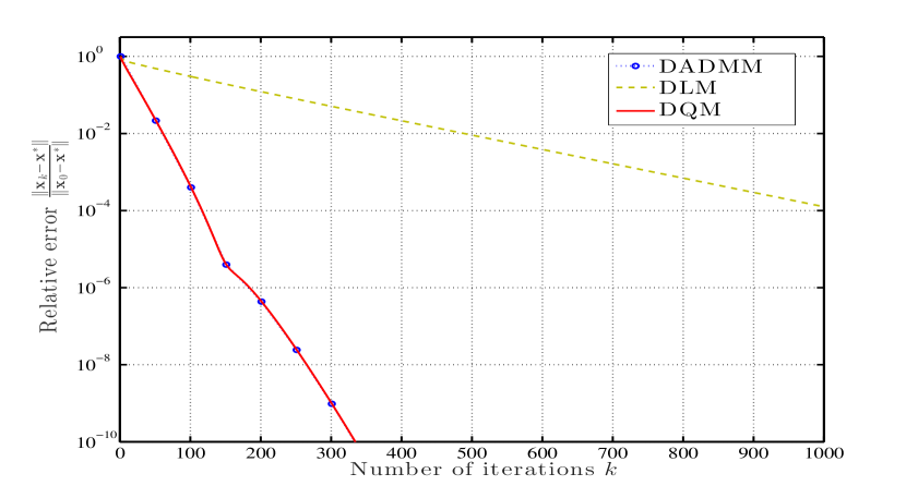
Figure 1: Relative error ${\|{\mathbf{x}}_{k}-{\mathbf{x}}^{*}\|}/{\|{\mathbf{x}}_{0}-{\mathbf{x}}^{*}\|}$ of DADMM, DQM, and DLM versus number of iterations for a random network of size $n=10$. The convergence path of DQM is similar to the one for DADMM and they outperform DLM by orders of magnitude.

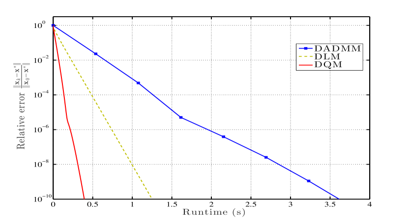
Figure 2: Relative error ${\|{\mathbf{x}}_{k}-{\mathbf{x}}^{*}\|}/{\|{\mathbf{x}}_{0}-{\mathbf{x}}^{*}\|}$ of DADMM, DQM, and DLM versus runtime for the setting in Fig. 1. The computational cost of DQM is lower than DADMM and DLM.

We compare the convergence paths of the DLM, DQM, and DADMM algorithms for solving the logistic regression problem in (38). Edges between the nodes are randomly generated with the connectivity ratio $r_{c}$. Observe that the connectivity ratio $r_{c}$ is the probability of two nodes being connected.

In the first experiment we set the number of nodes as $n=10$ and the connectivity ratio as $r_{\mathrm{c}}=0.4$. Each agent holds $q=5$ samples and the dimension of feature vectors is $p=3$. Fig. 1 illustrates the relative errors ${\|{\mathbf{x}}_{k}-{\mathbf{x}}^{*}\|}/{\|{\mathbf{x}}_{0}-{\mathbf{x}}^{*}\|}$ for DLM, DQM, and DADMM versus the number of iterations. Notice that the parameter $c$ for the three methods is optimized by $c_{\mathrm{ADMM}}=0.7$, $c_{\mathrm{DLM}}=5.5$, and $c_{\mathrm{DQM}}=0.7$. The convergence path of DQM is almost identical to the convergence path of DADMM. Moreover, DQM outperforms DLM by orders of magnitude. To be more precise, the relative errors ${\|{\mathbf{x}}_{k}-{\mathbf{x}}^{*}\|}/{\|{\mathbf{x}}_{0}-{\mathbf{x}}^{*}\|}$ for DQM and DADMM after $k=300$ iterations are below $10^{-9}$, while for DLM the relative error after the same number of iterations is $5\times 10^{-2}$. Conversely, achieving accuracy ${\|{\mathbf{x}}_{k}-{\mathbf{x}}^{*}\|}/{\|{\mathbf{x}}_{0}-{\mathbf{x}}^{*}\|}=10^{-3}$ for DQM and DADMM requires $91$ iterations, while DLM requires $758$ iterations to reach the same accuracy. Hence, the number of iterations that DLM requires to achieve a specific accuracy is $8$ times more than the one for DQM.

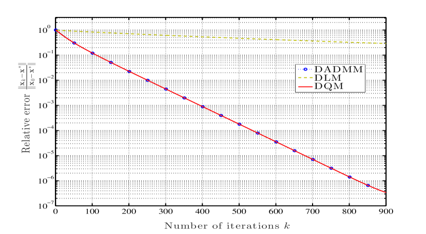
Figure 3: Relative error ${\|{\mathbf{x}}_{k}-{\mathbf{x}}^{*}\|}/{\|{\mathbf{x}}_{0}-{\mathbf{x}}^{*}\|}$ of DADMM, DQM, and DLM versus number of iterations for a random network of size $n=100$. The performances of DQM and DADMM are still similar. DLM is impractical in this setting.

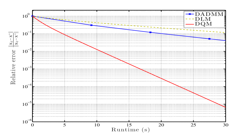
Figure 4: Relative error ${\|{\mathbf{x}}_{k}-{\mathbf{x}}^{*}\|}/{\|{\mathbf{x}}_{0}-{\mathbf{x}}^{*}\|}$ of DADMM, DQM, and DLM versus runtime for the setting in Fig. 2. The convergence time of DADMM is slightly faster relative to DLM, while DQM is the most efficient method among these three algorithms.

Observe that the computational complexity of DQM is lower than DADMM. Therefore, DQM outperforms DADMM in terms of convergence time or number of required operations until convergence. This phenomenon is shown in Fig 2 by comparing the relative of errors of DLM, DQM, and DADMM versus CPU runtime. According to Fig 2, DADMM achieves the relative error ${\|{\mathbf{x}}_{k}-{\mathbf{x}}^{*}\|}/{\|{\mathbf{x}}_{0}-{\mathbf{x}}^{*}\|}=10^{-10}$ after running for $3.6$ seconds, while DLM and DQM require $1.3$ and $0.4$ seconds, respectively, to achieve the same accuracy.

We also compare the performances of DLM, DQM, and DADMM in a larger scale logistic regression problem by setting size of network $n=100$, number of sample points at each node $q=20$, and dimension of feature vectors $p=10$. We keep the rest of the parameters as in Fig. 1. Convergence paths of the relative errors ${\|{\mathbf{x}}_{k}-{\mathbf{x}}^{*}\|}/{\|{\mathbf{x}}_{0}-{\mathbf{x}}^{*}\|}$ for DLM, DQM, and DADMM versus the number of iterations are illustrated in Fig. 3. Different choices of parameter $c$ are considered for these algorithms and the best for each is chosen for the final comparison. The optimal choices of parameter $c$ for DADMM, DLM, and DQM are $c_{\mathrm{ADMM}}=0.68$, $c_{\mathrm{DLM}}=12.3$, and $c_{\mathrm{DQM}}=0.68$, respectively. The results for the large scale problem in Fig. 3 are similar to the results in Fig. 1. We observe that DQM performs as well as DADMM, while both outperform DLM. To be more precise, DQM and DADMM after $k=900$ iterations reach the relative error ${\|{\mathbf{x}}_{k}-{\mathbf{x}}^{*}\|}/{\|{\mathbf{x}}_{0}-{\mathbf{x}}^{*}\|}=3.4\times 10^{-7}$, while the relative error of DLM after the same number of iterations is $2.9\times 10^{-1}$. Conversely, achieving the accuracy ${\|{\mathbf{x}}_{k}-{\mathbf{x}}^{*}\|}/{\|{\mathbf{x}}_{0}-{\mathbf{x}}^{*}\|}=0.3$ for DQM and DADMM requires $52$ iterations, while DLM requires $870$ iterations to reach the same accuracy. Hence, in this setting the number of iterations that DLM requires to achieve a specific accuracy is $16$ times more than the one for DQM. These numbers show that the advantages of DQM relative to DLM are more significant in large scale problems.

Notice that in large scale logistic regression problems we expect larger condition number for the objective function $f$. In these scenarios we expect to observe a poor performance by the DLM algorithm that only operates on first-order information. This expectation is satisfied by comparing the relative errors of DLM, DQM, and DADMM versus runtime for the large scale problem in Fig. 4. In this case, DLM is even worse than DADMM that has a very high computational complexity. Similar to the result in Fig. 3, DQM has the best performance among these three methods.

V-B Effect of the regularization parameter $c$

The parameter $c$ has a significant role in the convergence of DADMM. Likewise, choosing the optimal choice of $c$ is critical in the convergence of DQM. We study the effect of $c$ by tuning this parameter for a fixed network and training set. We use all the parameters in Fig. 1 and we compare performance of the DQM algorithm for the values $c=0.2$, $c=0.4$, $c=0.8$, and $c=1$. Fig. 5 illustrates the convergence paths of the DQM algorithm for different choices of the parameter $c$. The best performance among these choices is achieved for $c=0.8$. The comparison of the plots in Fig. 5 shows that increasing or decreasing the parameter $c$ is not necessarily leads to a faster convergence. We can interpret $c$ as the stepsize of DQM which the optimal choice may vary for the problems with different network sizes, network topologies, condition numbers of objective functions, etc.

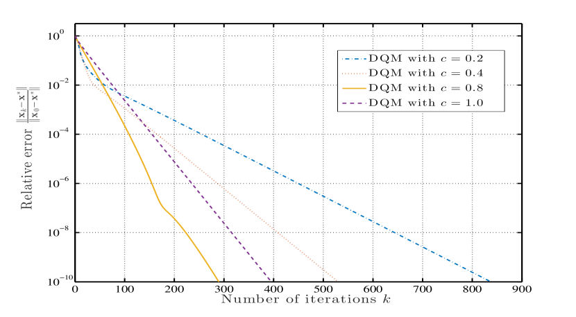
Figure 5: Relative error ${\|{\mathbf{x}}_{k}-{\mathbf{x}}^{*}\|}/{\|{\mathbf{x}}_{0}-{\mathbf{x}}^{*}\|}$ of DQM for parameters $c=0.2$, $c=0.4$, $c=0.8$, and $c=1$ when the network is formed by $n=10$ nodes and the connectivity ratio is $r_{c}=0.4$. The best performance belongs to $c=0.8$.

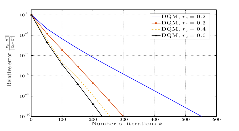
Figure 6: Relative error ${\|{\mathbf{x}}_{k}-{\mathbf{x}}^{*}\|}/{\|{\mathbf{x}}_{0}-{\mathbf{x}}^{*}\|}$ of DQM for random graphs with different connectivity ratios $r_{c}$. The linear convergence of DQM accelerates by increasing the connectivity ratio.

V-C Effect of network topology

According to (31) the constant of linear convergence for DQM depends on the bounds for the singular values of the oriented and unoriented incidence matrices ${\mathbf{E}}_{o}$ and ${\mathbf{E}}_{u}$. These bounds are related to the connectivity ratio of network. We study how the network topology affects the convergence speed of DQM. We use different values for the connectivity ratio to generate random graphs with different number of edges. In this experiment we use the connectivity ratios $r_{c}=\{0.2,0.3,0.4,0.6\}$ to generate the networks. The rest of the parameters are the same as the parameters in Fig. 1. Notice that since the connectivity parameters of these graphs are different, the optimal choices of $c$ for these graphs are different. The convergence paths of DQM with the connectivity ratios $r_{c}=\{0.2,0.3,0.4,0.6\}$ are shown in Fig. 6. The optimal choices of the parameter $c$ for these graphs are $c_{\mathrm{0.2}}=0.28$, $c_{\mathrm{0.3}}=0.25$, $c_{\mathrm{0.4}}=0.31$, and $c_{\mathrm{0.6}}=0.28$, respectively. Fig. 6 shows that the linear convergence of DQM accelerates by increasing the connectivity ratio of the graph.

VI Conclusions

A decentralized quadratically approximated version of the alternating direction method of multipliers (DQM) is proposed for solving decentralized optimization problems where components of the objective function are available at different nodes of a network. DQM minimizes a quadratic approximation of the convex problem that DADMM solves exactly at each step, and hence reduces the computational complexity of DADMM. Under some mild assumptions, linear convergence of the sequence generated by DQM is proven. Moreover, the constant of linear convergence for DQM approaches that of DADMM asymptotically. Numerical results for a logistic regression problem verify the analytical results that convergence paths of DQM and DADMM are similar for large iteration index, while the computational complexity of DQM is significantly smaller than DADMM.

Appendix A Proof of Lemma 1

According to the update for the Lagrange multiplier $\boldsymbol{\lambda}$ in (III), we can substitute $\boldsymbol{\lambda}_{k}$ by $\boldsymbol{\lambda}_{k+1}-c\left({\mathbf{A}}{\mathbf{x}}_{k+1}+{\mathbf{B}}{\mathbf{z}}_{k+1}\right)$. Applying this substitution into the first equation of (III) leads to

$${\mathbf{B}}^{T}\boldsymbol{\lambda}_{k+1}={\mathbf{0}}.$$ (40)

Observing the definitions ${\mathbf{B}}=[-{\mathbf{I}}_{mp};-{\mathbf{I}}_{mp}]$ and $\boldsymbol{\lambda}=[\boldsymbol{\alpha};\boldsymbol{\beta}]$, and the result in (40), we obtain $\boldsymbol{\alpha}_{k+1}=-\boldsymbol{\beta}_{k+1}$ for $k\geq 0$. Considering the initial condition $\boldsymbol{\alpha}_{0}=-\boldsymbol{\beta}_{0}$, we obtain that $\boldsymbol{\alpha}_{k}=-\boldsymbol{\beta}_{k}$ for $k\geq 0$ which follows the first claim in Lemma 1.

Based on the definitions ${\mathbf{A}}=[{\mathbf{A}}_{s};{\mathbf{A}}_{d}]$, ${\mathbf{B}}=[-{\mathbf{I}}_{mp};-{\mathbf{I}}_{mp}]$, and $\boldsymbol{\lambda}=[\boldsymbol{\alpha};\boldsymbol{\beta}]$, we can split the update for the Lagrange multiplier $\boldsymbol{\lambda}$ in (8) as

$$\boldsymbol{\alpha}_{k+1} =\boldsymbol{\alpha}_{k}+c[{\mathbf{A}}_{s}{\mathbf{x}}_{k+1}-{\mathbf{z}}_{k+1}],$$ (41)

$$\boldsymbol{\beta}_{k+1} =\boldsymbol{\beta}_{k}+c[{\mathbf{A}}_{d}{\mathbf{x}}_{k+1}-{\mathbf{z}}_{k+1}].$$ (42)

Observing the result that $\boldsymbol{\alpha}_{k}=-\boldsymbol{\beta}_{k}$ for $k\geq 0$, summing up the equations in (41) and (42) yields

$$({\mathbf{A}}_{s}+{\mathbf{A}}_{d}){\mathbf{x}}_{k+1}=2{\mathbf{z}}_{k+1}.$$ (43)

Considering the definition of the oriented incidence matrix ${\mathbf{E}}_{u}={\mathbf{A}}_{s}+{\mathbf{A}}_{d}$, we obtain that ${\mathbf{E}}_{u}{\mathbf{x}}_{k}=2{\mathbf{z}}_{k}$ holds for $k>0$. According to the initial condition ${\mathbf{E}}_{u}{\mathbf{x}}_{0}=2{\mathbf{z}}_{0}$, we can conclude that the relation ${\mathbf{E}}_{u}{\mathbf{x}}_{k}=2{\mathbf{z}}_{k}$ holds for $k\geq 0$.

Subtract the update for $\boldsymbol{\beta}_{k}$ in (42) from the update for $\boldsymbol{\alpha}_{k}$ in (41) and consider the relation $\boldsymbol{\beta}_{k}=-\boldsymbol{\alpha}_{k}$ to obtain

$$\boldsymbol{\alpha}_{k+1}=\boldsymbol{\alpha}_{k}+\frac{c}{2}({\mathbf{A}}_{s}-{\mathbf{A}}_{d}){\mathbf{x}}_{k+1}.$$ (44)

Substituting ${\mathbf{A}}_{s}-{\mathbf{A}}_{d}$ in (44) by ${\mathbf{E}}_{o}$ implies that

$$\boldsymbol{\alpha}_{k+1}=\boldsymbol{\alpha}_{k}+\frac{c}{2}{\mathbf{E}}_{o}{\mathbf{x}}_{k+1}.$$ (45)

Hence, if $\boldsymbol{\alpha}_{k}$ lies in the column space of matrix ${\mathbf{E}}_{o}$, then $\boldsymbol{\alpha}_{k+1}$ also lies in the column space of ${\mathbf{E}}_{o}$. According to the third condition of Assumption 1, $\boldsymbol{\alpha}_{0}$ satisfies this condition, therefore $\boldsymbol{\alpha}_{k}$ lies in the column space of matrix ${\mathbf{E}}_{o}$ for all $k\geq 0$.

Appendix B Proof of Proposition 1

The update for the multiplier $\boldsymbol{\lambda}$ in (8) implies that we can substitute $\boldsymbol{\lambda}_{k}$ by $\boldsymbol{\lambda}_{k+1}-c({\mathbf{A}}{\mathbf{x}}_{k+1}+{\mathbf{B}}{\mathbf{z}}_{k+1})$ to simplify (12) as

$$\nabla f({\mathbf{x}}_{k})+{\mathbf{H}}_{k}({\mathbf{x}}_{k+1}-{\mathbf{x}}_{k})+{\mathbf{A}}^{T}\boldsymbol{\lambda}_{k+1}+c{\mathbf{A}}^{T}{\mathbf{B}}\left({\mathbf{z}}_{k}-{\mathbf{z}}_{k+1}\right)={\mathbf{0}}.$$ (46)

Considering the first result of Lemma 1 that $\boldsymbol{\alpha}_{k}=-\boldsymbol{\beta}_{k}$ for $k\geq 0$ in association with the definition ${\mathbf{A}}=[{\mathbf{A}}_{s};{\mathbf{A}}_{d}]$ implies that the product ${\mathbf{A}}^{T}\boldsymbol{\lambda}_{k+1}$ is equivalent to

$${\mathbf{A}}^{T}\boldsymbol{\lambda}_{k+1}={\mathbf{A}}_{s}^{T}\boldsymbol{\alpha}_{k+1}+{\mathbf{A}}_{d}^{T}\boldsymbol{\beta}_{k+1}=({\mathbf{A}}_{s}-{\mathbf{A}}_{d})^{T}\boldsymbol{\alpha}_{k+1}.$$ (47)

According to the definition ${\mathbf{E}}_{o}:={\mathbf{A}}_{s}-{\mathbf{A}}_{d}$, the right hand side of (47) can be simplified as

$${\mathbf{A}}^{T}\boldsymbol{\lambda}_{k+1}={\mathbf{E}}_{o}^{T}\boldsymbol{\alpha}_{k+1}.$$ (48)

Based on the structures of the matrices ${\mathbf{A}}$ and ${\mathbf{B}}$, and the definition ${\mathbf{E}}_{u}:={\mathbf{A}}_{s}+{\mathbf{A}}_{d}$, we can simplify ${\mathbf{A}}^{T}{\mathbf{B}}$ as

$${\mathbf{A}}^{T}{\mathbf{B}}=-{\mathbf{A}}_{s}^{T}-{\mathbf{A}}_{d}^{T}=-{\mathbf{E}}_{u}^{T}.$$ (49)

Substituting the results in (48) and (49) into (46) leads to

$$\nabla f({\mathbf{x}}_{k})+{\mathbf{H}}_{k}({\mathbf{x}}_{k+1}-{\mathbf{x}}_{k})+{\mathbf{E}}_{o}^{T}\boldsymbol{\alpha}_{k+1}+c{\mathbf{E}}_{u}^{T}\left({\mathbf{z}}_{k+1}-{\mathbf{z}}_{k}\right)={\mathbf{0}}.$$ (50)

The second result in Lemma 1 states that ${\mathbf{z}}_{k}={\mathbf{E}}_{u}{\mathbf{x}}_{k}/2$. Multiplying both sides of this equality by ${\mathbf{E}}_{u}^{T}$ from left we obtain that ${\mathbf{E}}_{u}^{T}{\mathbf{z}}_{k}={\mathbf{E}}_{u}^{T}{\mathbf{E}}_{u}{\mathbf{x}}_{k}/2$ for $k\geq 0$. Observing the definition of the unoriented Laplacian ${\mathbf{L}}_{u}:={\mathbf{E}}_{u}^{T}{\mathbf{E}}_{u}/2$, we obtain that the product ${\mathbf{E}}_{u}^{T}{\mathbf{z}}_{k}$ is equal to ${\mathbf{L}}_{u}{\mathbf{x}}_{k}$ for $k\geq 0$. Therefore, in (50) we can substitute ${\mathbf{E}}_{u}^{T}\left({\mathbf{z}}_{k+1}-{\mathbf{z}}_{k}\right)$ by ${\mathbf{L}}_{u}({\mathbf{x}}_{k+1}-{\mathbf{x}}_{k})$ and write

$$\nabla f({\mathbf{x}}_{k})+\left({\mathbf{H}}_{k}+c{\mathbf{L}}_{u}\right)({\mathbf{x}}_{k+1}-{\mathbf{x}}_{k})+{\mathbf{E}}_{o}^{T}\boldsymbol{\alpha}_{k+1}={\mathbf{0}}.$$ (51)

Observe that the new variables $\boldsymbol{\phi}_{k}$ are defined as $\boldsymbol{\phi}_{k}:={\mathbf{E}}_{o}^{T}\boldsymbol{\alpha}_{k}$. Multiplying both sides of (45) by ${\mathbf{E}}_{o}^{T}$ from the left hand side and considering the definition of oriented Laplacian ${\mathbf{L}}_{o}={\mathbf{E}}_{o}^{T}{\mathbf{E}}_{o}/2$ follows the update rule of $\boldsymbol{\phi}_{k}$ in (1), i.e.,

$$\boldsymbol{\phi}_{k+1}=\boldsymbol{\phi}_{k}+c{\mathbf{L}}_{o}{\mathbf{x}}_{k+1}.$$ (52)

According to the definition $\boldsymbol{\phi}_{k}={\mathbf{E}}_{o}^{T}\boldsymbol{\alpha}_{k}$ and the update formula in (52), we can conclude that ${\mathbf{E}}_{o}^{T}\boldsymbol{\alpha}_{k+1}=\boldsymbol{\phi}_{k+1}=\boldsymbol{\phi}_{k}+c{\mathbf{L}}_{o}{\mathbf{x}}_{k+1}$. Substituting ${\mathbf{E}}_{o}^{T}\boldsymbol{\alpha}_{k+1}$ by $\boldsymbol{\phi}_{k}+c{\mathbf{L}}_{o}{\mathbf{x}}_{k+1}$ in (51) yields

$$\nabla f({\mathbf{x}}_{k})+\left({\mathbf{H}}_{k}+c{\mathbf{L}}_{u}\right)({\mathbf{x}}_{k+1}-{\mathbf{x}}_{k})+\boldsymbol{\phi}_{k}+c{\mathbf{L}}_{o}{\mathbf{x}}_{k+1}={\mathbf{0}}.$$ (53)

Observing the definition ${\mathbf{D}}=({\mathbf{L}}_{u}+{\mathbf{L}}_{o})/2$ we rewrite (53) as

$$\left({\mathbf{H}}_{k}+2c{\mathbf{D}}\right){\mathbf{x}}_{k+1}=\left({\mathbf{H}}_{k}+c{\mathbf{L}}_{u}\right){\mathbf{x}}_{k}-\nabla f({\mathbf{x}}_{k})-\boldsymbol{\phi}_{k}.$$ (54)

Multiplying both sides of (54) by $\left({\mathbf{H}}_{k}+2c{\mathbf{D}}\right)^{-1}$ from the left hand side yields the first update in (1).

Appendix C Proof of Lemma 2

Consider two arbitrary vectors ${\mathbf{x}}:=[{\mathbf{x}}_{1};\dots;{\mathbf{x}}_{n}]\in{\mathbb{R}}^{np}$ and ${\hat{\mathbf{x}}}:=[{\hat{\mathbf{x}}}_{1};\dots;{\hat{\mathbf{x}}}_{n}]\in{\mathbb{R}}^{np}$. Since the aggregate function Hessian is block diagonal where the $i$-th diagonal block is given by $\nabla^{2}f_{i}({\mathbf{x}}_{i})$, we obtain that the difference of Hessians ${\mathbf{H}}({\mathbf{x}})-{\mathbf{H}}({\hat{\mathbf{x}}})$ is also block diagonal where the $i$-th diagonal block ${{\mathbf{H}}({\mathbf{x}})_{ii}-{\mathbf{H}}({\hat{\mathbf{x}}})}_{ii}$ is

$${{\mathbf{H}}({\mathbf{x}})_{ii}-{\mathbf{H}}({\hat{\mathbf{x}}})}_{ii}=\nabla^{2}f_{i}({\mathbf{x}}_{i})-\nabla^{2}f_{i}({\hat{\mathbf{x}}}_{i}).$$ (55)

Consider any vector ${\mathbf{v}}\in{\mathbb{R}}^{np}$ and separate each $p$ components of vector ${\mathbf{v}}$ and consider it as a new vector called ${\mathbf{v}}_{i}\in{\mathbb{R}}^{p}$, i.e., ${\mathbf{v}}:=[{\mathbf{v}}_{1};\dots;{\mathbf{v}}_{n}]$. Observing the relation for the difference ${\mathbf{H}}({\mathbf{x}})-{\mathbf{H}}({\hat{\mathbf{x}}})$ in (55), the symmetry of matrices ${\mathbf{H}}({\mathbf{x}})$ and ${\mathbf{H}}({\hat{\mathbf{x}}})$, and the definition of Euclidean norm of a matrix that $\|{\mathbf{A}}\|=\sqrt{\lambda_{max}({\mathbf{A}}^{T}{\mathbf{A}})}$, we obtain that the squared difference norm $\|{\mathbf{H}}({\mathbf{x}})-{\mathbf{H}}({\hat{\mathbf{x}}})\|^{2}$ can be written as

$$\left\|{\mathbf{H}}({\mathbf{x}})-{\mathbf{H}}({\hat{\mathbf{x}}})\right\|^{2}\! =\max_{{\mathbf{v}}}\frac{{\mathbf{v}}^{T}[{\mathbf{H}}({\mathbf{x}})-{\mathbf{H}}({\hat{\mathbf{x}}})]^{2}{\mathbf{v}}}{\|{\mathbf{v}}\|^{2}}$$ (56)

$$=\max_{{\mathbf{v}}}\frac{\sum_{i=1}^{n}{\mathbf{v}}_{i}^{T}\left[\nabla^{2}f_{i}({\mathbf{x}}_{i})-\nabla^{2}f_{i}({\hat{\mathbf{x}}}_{i})\right]^{2}{\mathbf{v}}_{i}}{\|{\mathbf{v}}\|^{2}}$$

Using the Cauchy-Schwarz inequality we can write

$${\mathbf{v}}_{i}^{T}\!\left[\nabla^{2}f_{i}({\mathbf{x}}_{i})\!-\!\nabla^{2}f_{i}({\hat{\mathbf{x}}}_{i})\right]^{2}\!{\mathbf{v}}_{i}\leq\left\|\nabla^{2}f_{i}({\mathbf{x}}_{i})\!-\!\nabla^{2}f_{i}({\hat{\mathbf{x}}}_{i})\right\|^{2}\!\|{\mathbf{v}}_{i}\|^{2}$$ (57)

Substituting the upper bound in (57) into (56) implies that the squared norm $\left\|{\mathbf{H}}({\mathbf{x}})-{\mathbf{H}}({\hat{\mathbf{x}}})\right\|^{2}$ is bounded above as

$$\left\|{\mathbf{H}}({\mathbf{x}})-{\mathbf{H}}({\hat{\mathbf{x}}})\right\|^{2}\leq\max_{{\mathbf{v}}}\frac{\sum_{i=1}^{n}\left\|\nabla^{2}f_{i}({\mathbf{x}}_{i})-\nabla^{2}f_{i}({\hat{\mathbf{x}}}_{i})\right\|^{2}\|{\mathbf{v}}_{i}\|^{2}}{\|{\mathbf{v}}\|^{2}}.$$ (58)

Observe that Assumption 3 states that local objective functions Hessian $\nabla^{2}f_{i}({\mathbf{x}}_{i})$ are Lipschitz continuous with constant $L$, i.e. $\|\nabla^{2}f_{i}({\mathbf{x}}_{i})-\nabla^{2}f_{i}({\hat{\mathbf{x}}}_{i})\|\leq L\|{\mathbf{x}}_{i}-{\hat{\mathbf{x}}}_{i}\|$. Considering this inequality the upper bound in (58) can be changed by replacing $\|\nabla^{2}f_{i}({\mathbf{x}}_{i})-\nabla^{2}f_{i}({\hat{\mathbf{x}}}_{i})\|$ by $L\|{\mathbf{x}}_{i}-{\hat{\mathbf{x}}}_{i}\|$ which yields

$$\left\|{\mathbf{H}}({\mathbf{x}})-{\mathbf{H}}({\hat{\mathbf{x}}})\right\|^{2}\leq\max_{{\mathbf{v}}}\frac{L^{2}\sum_{i=1}^{n}\left\|{\mathbf{x}}_{i}-{\hat{\mathbf{x}}}_{i}\right\|^{2}\|{\mathbf{v}}_{i}\|^{2}}{\sum_{i=1}^{n}\|{\mathbf{v}}_{i}\|^{2}}.$$ (59)

Note that for any sequences of scalars such as $a_{i}$ and $b_{i}$, the inequality $\sum_{i=1}^{n}a_{i}^{2}b_{i}^{2}\leq(\sum_{i=1}^{n}a_{i}^{2})(\sum_{i=1}^{n}b_{i}^{2})$ holds. If we divide both sides of this relation by $\sum_{i=1}^{n}b_{i}^{2}$ and set $a_{i}=\|{\mathbf{x}}_{i}-{\hat{\mathbf{x}}}_{i}\|$ and $b_{i}=\|{\mathbf{v}}_{i}\|$, we obtain

$$\frac{\sum_{i=1}^{n}\left\|{\mathbf{x}}_{i}-{\hat{\mathbf{x}}}_{i}\right\|^{2}\|{\mathbf{v}}_{i}\|^{2}}{\sum_{i=1}^{n}\|{\mathbf{v}}_{i}\|^{2}}\leq\sum_{i=1}^{n}\left\|{\mathbf{x}}_{i}-{\hat{\mathbf{x}}}_{i}\right\|^{2}.$$ (60)

Combining the two inequalities in (59) and (60) leads to

$$\left\|{\mathbf{H}}({\mathbf{x}})-{\mathbf{H}}({\hat{\mathbf{x}}})\right\|^{2}\leq\max_{{\mathbf{v}}}L^{2}\sum_{i=1}^{n}\left\|{\mathbf{x}}_{i}-{\hat{\mathbf{x}}}_{i}\right\|^{2}.$$ (61)

Since the right hand side of (61) does not depend on ${\mathbf{v}}$ we can eliminate the maximization with respect to ${\mathbf{v}}$. Further, note that according to the structure of vectors ${\mathbf{x}}$ and ${\hat{\mathbf{x}}}$, we can write $\left\|{\mathbf{x}}-{\hat{\mathbf{x}}}\right\|^{2}=\sum_{i=1}^{n}\left\|{\mathbf{x}}_{i}-{\hat{\mathbf{x}}}_{i}\right\|^{2}$. These two observations in association with (61) imply that

$$\left\|{\mathbf{H}}({\mathbf{x}})-{\mathbf{H}}({\hat{\mathbf{x}}})\right\|^{2}\leq L^{2}\left\|{\mathbf{x}}-{\hat{\mathbf{x}}}\right\|^{2},$$ (62)

Computing the square roots of terms in (62) yields (20).

Appendix D Proofs of Propositions 2 and 3

The fundamental theorem of calculus implies that the difference of gradients $\nabla f({\mathbf{x}}_{k+1})-\nabla f({\mathbf{x}}_{k})$ can be written as

$$\nabla f({\mathbf{x}}_{k+1})-\nabla f({\mathbf{x}}_{k})=\int_{0}^{1}{\mathbf{H}}(s{\mathbf{x}}_{k+1}+(1-s){\mathbf{x}}_{k})({\mathbf{x}}_{k+1}-{\mathbf{x}}_{k})\ ds.$$ (63)

By computing norms of both sides of (63) and considering that norm of integral is smaller than integral of norm we obtain that

$$\|\nabla f({\mathbf{x}}_{k+1})-\nabla f({\mathbf{x}}_{k})\|\!\leq\!\!\int_{0}^{1}\!\!\!\!\|{\mathbf{H}}(s{\mathbf{x}}_{k+1}+(1-s){\mathbf{x}}_{k})({\mathbf{x}}_{k+1}-{\mathbf{x}}_{k})\|ds.$$ (64)

The upper bound $M$ for the eigenvalues of the Hessians as in (19), implies that $\|{\mathbf{H}}\left(s{\mathbf{x}}+(1-s){\hat{\mathbf{x}}}\right)({\mathbf{x}}-{\hat{\mathbf{x}}})\|\leq M\|{\mathbf{x}}-{\hat{\mathbf{x}}}\|$. Substituting this upper bound into (64) leads to

$$\|\nabla f({\mathbf{x}}_{k+1})-\nabla f({\mathbf{x}}_{k})\|\leq M\|{\mathbf{x}}_{k+1}-{\mathbf{x}}_{k}\|.$$ (65)

The error vector norm $\|{\mathbf{e}}_{k}^{DLM}\|$ in (34) is bounded above as

$$\|{\mathbf{e}}_{k}^{DLM}\|\leq\|\nabla f({\mathbf{x}}_{k+1})-\nabla f({\mathbf{x}}_{k})\|+\rho\|{\mathbf{x}}_{k+1}-{\mathbf{x}}_{k}\|.$$ (66)

By substituting the upper bound for $\|\nabla f({\mathbf{x}}_{k+1})-\nabla f({\mathbf{x}}_{k})\|$ in (65) into (66), the claim in (35) follows.

To prove (22), first we show that $\|{\mathbf{e}}_{k}^{DQM}\|\leq 2M\|{\mathbf{x}}_{k+1}-{\mathbf{x}}_{k}\|$ holds. Observe that the norm of error vector ${\mathbf{e}}_{k}^{DQM}$ defined (21) can be upper bounded using the triangle inequality as

$$\|{\mathbf{e}}_{k}^{DQM}\|\leq\|\nabla f({\mathbf{x}}_{k+1})-\nabla f({\mathbf{x}}_{k})\|+\|{\mathbf{H}}_{k}({\mathbf{x}}_{k+1}-{\mathbf{x}}_{k})\|.$$ (67)

Based on the Cauchy-Schwarz inequality and the upper bound $M$ for the eigenvalues of Hessians as in (19), we obtain $\|{\mathbf{H}}_{k}({\mathbf{x}}_{k+1}-{\mathbf{x}}_{k})\|\leq M\|{\mathbf{x}}_{k+1}-{\mathbf{x}}_{k}\|$. Further, as mentioned in (65) the difference of gradients $\|\nabla f({\mathbf{x}}_{k+1})-\nabla f({\mathbf{x}}_{k})\|$ is upper bounded by $M\|{\mathbf{x}}_{k+1}-{\mathbf{x}}_{k}\|$. Substituting these upper bounds for the terms in the right hand side of (67) yields

$$\|{\mathbf{e}}_{k}^{DQM}\|\leq 2M\|{\mathbf{x}}_{k+1}-{\mathbf{x}}_{k}\|.$$ (68)

The next step is to show that $\|{\mathbf{e}}_{k}^{DQM}\|\leq(L/2)\|{\mathbf{x}}_{k+1}-{\mathbf{x}}_{k}\|^{2}$. Adding and subtracting the integral $\int_{0}^{1}{\mathbf{H}}({\mathbf{x}}_{k})({\mathbf{x}}_{k+1}-{\mathbf{x}}_{k})\ ds$ to the right hand side of (63) results in

$$\nabla f({\mathbf{x}}_{k+1})-\nabla f({\mathbf{x}}_{k})=\int_{0}^{1}{\mathbf{H}}({\mathbf{x}}_{k})({\mathbf{x}}_{k+1}-{\mathbf{x}}_{k})\ ds$$

$$+\int_{0}^{1}\left[{\mathbf{H}}(s{\mathbf{x}}_{k+1}+(1-s){\mathbf{x}}_{k})-{\mathbf{H}}({\mathbf{x}}_{k})\right]({\mathbf{x}}_{k+1}-{\mathbf{x}}_{k})\ ds.$$ (69)

First observe that the integral $\int_{0}^{1}{\mathbf{H}}({\mathbf{x}}_{k})({\mathbf{x}}_{k+1}-{\mathbf{x}}_{k})\ ds$ can be simplified as ${\mathbf{H}}({\mathbf{x}}_{k})({\mathbf{x}}_{k+1}-{\mathbf{x}}_{k})$. Observing this simplification and regrouping the terms yield

$$\nabla f({\mathbf{x}}_{k+1})-\nabla f({\mathbf{x}}_{k})-{\mathbf{H}}({\mathbf{x}}_{k})({\mathbf{x}}_{k+1}-{\mathbf{x}}_{k})=$$

$$\int_{0}^{1}\left[{\mathbf{H}}(s{\mathbf{x}}_{k+1}+(1-s){\mathbf{x}}_{k})-{\mathbf{H}}({\mathbf{x}}_{k})\right]({\mathbf{x}}_{k+1}-{\mathbf{x}}_{k})\ ds.$$ (70)

Computing norms of both sides of (D), considering the fact that norm of integral is smaller than integral of norm, and using Cauchy-Schwarz inequality lead to

$$\|\nabla f({\mathbf{x}}_{k+1})-\nabla f({\mathbf{x}}_{k})-{\mathbf{H}}({\mathbf{x}}_{k})({\mathbf{x}}_{k+1}-{\mathbf{x}}_{k})\|\leq$$ (71)

$$\int_{0}^{1}\left\|{\mathbf{H}}(s{\mathbf{x}}_{k+1}+(1-s){\mathbf{x}}_{k})-{\mathbf{H}}({\mathbf{x}}_{k})\right\|\|{\mathbf{x}}_{k+1}-{\mathbf{x}}_{k}\|ds.$$

Lipschitz continuity of the Hessian as in (20) implies that $\left\|{\mathbf{H}}(s{\mathbf{x}}_{k+1}+(1-s){\mathbf{x}}_{k})-{\mathbf{H}}({\mathbf{x}}_{k})\right\|\leq sL\|{\mathbf{x}}_{k+1}-{\mathbf{x}}_{k}\|$. By substituting this upper bound into the integral in (71) and substituting the left hand side of (71) by $\|{\mathbf{e}}_{k}^{DQM}\|$ we obtain

$$\|{\mathbf{e}}_{k}^{DQM}\|\leq\int_{0}^{1}sL\|{\mathbf{x}}_{k+1}-{\mathbf{x}}_{k}\|^{2}ds.$$ (72)

Simplification of the integral in (72) follows

$$\|{\mathbf{e}}_{k}^{DQM}\|\leq\frac{L}{2}\|{\mathbf{x}}_{k+1}-{\mathbf{x}}_{k}\|^{2}.$$ (73)

The results in (68) and (73) follow the claim in (22).

Appendix E Proof of Lemma 3

In this section we first introduce an equivalent version of Lemma 3 for the DLM algorithm. Then, we show the validity of both lemmata in a general proof.

Lemma 4

Consider DLM as defined by (7)-(II). If Assumption 1 holds true, then the optimal arguments ${\mathbf{x}}^{*}$, ${\mathbf{z}}^{*}$, and $\boldsymbol{\alpha}^{*}$ satisfy

$$\nabla f({\mathbf{x}}_{k+1})-\nabla f({\mathbf{x}}^{*})+{\mathbf{e}}_{k}^{DLM}+{\mathbf{E}}_{o}^{T}(\boldsymbol{\alpha}_{k+1}-\boldsymbol{\alpha}^{*})$$

$$-c{\mathbf{E}}_{u}^{T}\left({\mathbf{z}}_{k}-{\mathbf{z}}_{k+1}\right) ={\mathbf{0}},$$ (74)

$$2(\boldsymbol{\alpha}_{k+1}-\boldsymbol{\alpha}_{k})-{c}{\mathbf{E}}_{o}({\mathbf{x}}_{k+1}-{\mathbf{x}}^{*}) ={\mathbf{0}},$$ (75)

$${\mathbf{E}}_{u}({\mathbf{x}}_{k}-{\mathbf{x}}^{*})-2({\mathbf{z}}_{k}-{\mathbf{z}}^{*}) ={\mathbf{0}}.$$ (76)

Notice that the claims in Lemmata 3 and 4 are identical except in the error term of the first equalities. To provide a general framework to prove the claim in these lemmata we introduce ${\mathbf{e}}_{k}$ as the general error vector. By replacing ${\mathbf{e}}_{k}$ with ${\mathbf{e}}_{k}^{DQM}$ we obtain the result of DQM in Lemma 3 and by setting ${\mathbf{e}}_{k}={\mathbf{e}}_{k}^{DLM}$ the result in Lemma 4 follows. We start with the following Lemma that captures the KKT conditions of optimization problem (4).

Lemma 5

Consider the optimization problem (4). The optimal Lagrange multiplier $\boldsymbol{\alpha}^{*}$, primal variable ${\mathbf{x}}^{*}$ and auxiliary variable ${\mathbf{z}}^{*}$ satisfy the following system of equations

$$\nabla f({\mathbf{x}}^{*})+{\mathbf{E}}_{o}^{T}\boldsymbol{\alpha}^{*}={\mathbf{0}},\quad{\mathbf{E}}_{o}{\mathbf{x}}^{*}={\mathbf{0}},\quad{\mathbf{E}}_{u}{\mathbf{x}}^{*}=2{\mathbf{z}}^{*}.$$ (77)

Proof : First observe that the KKT conditions of the decentralized optimization problem in (4) are given by

$$\nabla f({\mathbf{x}}^{*})+{\mathbf{A}}^{T}{\boldsymbol{\lambda}^{*}}={\mathbf{0}},\quad{\mathbf{B}}^{T}{\boldsymbol{\lambda}^{*}}={\mathbf{0}},\quad{\mathbf{A}}{\mathbf{x}}^{*}+{\mathbf{B}}{\mathbf{z}}^{*}={\mathbf{0}}.$$ (78)

Based on the definitions of the matrix ${\mathbf{B}}=[-{\mathbf{I}}_{mp};-{\mathbf{I}}_{mp}]$ and the optimal Lagrange multiplier $\boldsymbol{\lambda}^{*}:=[\boldsymbol{\alpha}^{*};\boldsymbol{\beta}^{*}]$, we obtain that ${\mathbf{B}}^{T}{\boldsymbol{\lambda}^{*}}={\mathbf{0}}$ in (78) is equivalent to $\boldsymbol{\alpha}^{*}=-\boldsymbol{\beta}^{*}$. Considering this result and the definition ${\mathbf{A}}=[{\mathbf{A}}_{s};{\mathbf{A}}_{d}]$, we obtain

$${\mathbf{A}}^{T}{\boldsymbol{\lambda}^{*}}={\mathbf{A}}_{s}^{T}\boldsymbol{\alpha}^{*}+{\mathbf{A}}_{d}^{T}\boldsymbol{\beta}^{*}=({\mathbf{A}}_{s}-{\mathbf{A}}_{d})^{T}\boldsymbol{\alpha}^{*}.$$ (79)

The definition ${\mathbf{E}}_{o}:={\mathbf{A}}_{s}-{\mathbf{A}}_{d}$ implies that the right hand side of (79) can be simplified as ${\mathbf{E}}_{o}^{T}\boldsymbol{\alpha}^{*}$ which shows ${\mathbf{A}}^{T}{\boldsymbol{\lambda}^{*}}={\mathbf{E}}_{o}^{T}\boldsymbol{\alpha}^{*}$. Substituting ${\mathbf{A}}^{T}{\boldsymbol{\lambda}^{*}}$ by ${\mathbf{E}}_{o}^{T}\boldsymbol{\alpha}^{*}$ into the first equality in (78) follows the first claim in (77).

Decompose the KKT condition ${\mathbf{A}}{\mathbf{x}}^{*}+{\mathbf{B}}{\mathbf{z}}^{*}={\mathbf{0}}$ in (78) based on the definitions of ${\mathbf{A}}$ and ${\mathbf{B}}$ as

$${\mathbf{A}}_{s}{\mathbf{x}}^{*}-{\mathbf{z}}={\mathbf{0}},\quad{\mathbf{A}}_{d}{\mathbf{x}}^{*}-{\mathbf{z}}={\mathbf{0}}.$$ (80)

Subtracting the equalities in (80) implies that $({\mathbf{A}}_{s}-{\mathbf{A}}_{d}){\mathbf{x}}^{*}={\mathbf{0}}$ which by considering the definition ${\mathbf{E}}_{o}={\mathbf{A}}_{s}-{\mathbf{A}}_{d}$, the second equation in (77) follows. Summing up the equalities in (80) yields $({\mathbf{A}}_{s}+{\mathbf{A}}_{d}){\mathbf{x}}^{*}=2{\mathbf{z}}$. This observation in association with the definition ${\mathbf{E}}_{u}={\mathbf{A}}_{s}-{\mathbf{A}}_{d}$ follows the third equation in (77). $\blacksquare$

Proofs of Lemmata 3 and 4: First note that the results in Lemma 1 are also valid for DLM [22]. Now, consider the first order optimality condition for primal updates of DQM and DLM in (12) and (10), respectively. Further, recall the definitions of error vectors ${\mathbf{e}}_{k}^{DQM}$ and ${\mathbf{e}}_{k}^{DLM}$ in (21) and (34), respectively. Combining these observations we obtain that

$$\nabla f({\mathbf{x}}_{k+1})+{\mathbf{e}}_{k}+{\mathbf{A}}^{T}\boldsymbol{\lambda}_{k}+c{\mathbf{A}}^{T}\left({\mathbf{A}}{\mathbf{x}}_{k+1}+{\mathbf{B}}{\mathbf{z}}_{k}\right)={\mathbf{0}}.$$ (81)

Notice that by setting ${\mathbf{e}}_{k}={\mathbf{e}}_{k}^{DQM}$ we obtain the update for primal variable of DQM; likewise, setting ${\mathbf{e}}_{k}={\mathbf{e}}_{k}^{DLM}$ yields to the update of DLM.

Observe that the relation $\boldsymbol{\lambda}_{k}=\boldsymbol{\lambda}_{k+1}-c({\mathbf{A}}{\mathbf{x}}_{k+1}+{\mathbf{B}}{\mathbf{z}}_{k+1})$ holds for both DLM and DQM according to to the update formula for Lagrange multiplier in (8) and (III). Substituting $\boldsymbol{\lambda}_{k}$ by $\boldsymbol{\lambda}_{k+1}-c({\mathbf{A}}{\mathbf{x}}_{k+1}+{\mathbf{B}}{\mathbf{z}}_{k+1})$ in (81) follows

$$\nabla f({\mathbf{x}}_{k+1})+{\mathbf{e}}_{k}+{\mathbf{A}}^{T}\boldsymbol{\lambda}_{k+1}+c{\mathbf{A}}^{T}{\mathbf{B}}\left({\mathbf{z}}_{k}-{\mathbf{z}}_{k+1}\right)={\mathbf{0}}$$ (82)

Based on the result in Lemma 1, the components of the Lagrange multiplier $\boldsymbol{\lambda}=[\boldsymbol{\alpha};\boldsymbol{\beta}]$ satisfy $\boldsymbol{\alpha}_{k+1}=-\boldsymbol{\beta}_{k+1}$. Hence, the product ${\mathbf{A}}^{T}{\boldsymbol{\lambda}_{k+1}}$ can be simplified as ${\mathbf{A}}_{s}^{T}\boldsymbol{\alpha}_{k+1}-{\mathbf{A}}_{d}^{T}\boldsymbol{\alpha}_{k+1}={\mathbf{E}}_{o}^{T}\boldsymbol{\alpha}_{k+1}$ considering the definition that ${\mathbf{E}}_{o}={\mathbf{A}}_{s}-{\mathbf{A}}_{d}$. Furthermore, note that according to the definitions we have that ${\mathbf{A}}=[{\mathbf{A}}_{s};{\mathbf{A}}_{d}]$ and ${\mathbf{B}}=[-{\mathbf{I}};-{\mathbf{I}}]$ which implies that ${\mathbf{A}}^{T}{\mathbf{B}}=-({\mathbf{A}}_{s}+{\mathbf{A}}_{d})^{T}=-{\mathbf{E}}_{u}^{T}$. By making these substitutions into (82) we can write

$$\nabla f({\mathbf{x}}_{k+1})+{\mathbf{e}}_{k}+{\mathbf{E}}_{o}^{T}\boldsymbol{\alpha}_{k+1}-c{\mathbf{E}}_{u}^{T}\left({\mathbf{z}}_{k}-{\mathbf{z}}_{k+1}\right) ={\mathbf{0}}.$$ (83)

The first result in Lemma 5 is equivalent to $\nabla f({\mathbf{x}}^{*})+{\mathbf{E}}_{o}^{T}\boldsymbol{\alpha}^{*}={\mathbf{0}}$. Subtracting both sides of this equation from the relation in (83) follows the first claim of Lemmata 3 and 4.

We proceed to prove the second and third claims in Lemmata 3 and 4. The update formula for $\boldsymbol{\alpha}_{k}$ in (45) and the second result in Lemma 5 that ${\mathbf{E}}_{o}{\mathbf{x}}^{*}=0$ imply that the second claim of Lemmata 3 and 4 are valid. Further, the result in Lemma 1 guaranteaes that ${\mathbf{E}}_{u}{\mathbf{x}}_{k}=2{\mathbf{z}}_{k}$. This result in conjunction with the result in Lemma 5 that ${\mathbf{E}}_{u}{\mathbf{x}}^{*}=2{\mathbf{z}}^{*}$ leads to the third claim of Lemmata 3 and 4.

Appendix F Proofs of Theorems 1 and 2

To prove Theorems 1 and 2 we show a sufficient condition for the claims in these theorems. Then, we prove these theorems by showing validity of the sufficient condition. To do so, we use the general coefficient $\beta_{k}$ which is equivalent to $\zeta_{k}$ in the DQM algorithm and equivalent to $\rho+M$ in the DLM method. These definitions and the results in Propositions 2 and 3 imply that

$$\|{\mathbf{e}}_{k}\|\leq\beta_{k}\|{\mathbf{x}}_{k+1}-{\mathbf{x}}_{k}\|,$$ (84)

where ${\mathbf{e}}_{k}$ is ${\mathbf{e}}_{k}^{DQM}$ in DQM and ${\mathbf{e}}_{k}^{DLM}$ in DLM. The sufficient condition of Theorems 1 and 2 is studied in the following lemma.

Lemma 6

Consider the DLM and DQM algorithms as defined in (7)-(II) and (12)-(III), respectively. Further, conducer $\delta_{k}$ as a sequence of positive scalars. If Assumptions 1-4 hold true then the sequence $\|{\mathbf{u}}_{k}-{\mathbf{u}}^{*}\|_{\mathbf{C}}^{2}$ converges linearly as

$$\|{\mathbf{u}}_{k+1}-{\mathbf{u}}^{*}\|_{{\mathbf{C}}}^{2}\ \leq\ \frac{1}{1+\delta_{k}}\|{\mathbf{u}}_{k}-{\mathbf{u}}^{*}\|_{{\mathbf{C}}}^{2},$$ (85)

if the following inequality holds true,

$$\!\beta_{k}\|{\mathbf{x}}_{k+1}\!-\!{\mathbf{x}}^{*}\|\|{\mathbf{x}}_{k+1}\!-\!{\mathbf{x}}_{k}\|\!+\!\delta_{k}c\|{\mathbf{z}}_{k+1}\!-\!{\mathbf{z}}^{*}\|^{2}\!+\!\frac{\delta_{k}}{c}\|\boldsymbol{\alpha}_{k+1}\!-\!\boldsymbol{\alpha}^{*}\|^{2}$$

$$\leq m\|{\mathbf{x}}_{k+1}\!-\!{\mathbf{x}}^{*}\|^{2}+c\|{\mathbf{z}}_{k+1}\!-\!{\mathbf{z}}_{k}\|^{2}+\frac{1}{c}\|\boldsymbol{\alpha}_{k+1}\!-\!\boldsymbol{\alpha}_{k}\|^{2}.$$ (86)

Proof : Proving linear convergence of the sequence $\|{\mathbf{u}}_{k}-{\mathbf{u}}^{*}\|_{\mathbf{C}}^{2}$ as mentioned in (85) is equivalent to showing that

$$\delta_{k}\|{\mathbf{u}}_{k+1}-{\mathbf{u}}^{*}\|_{\mathbf{C}}^{2}\leq\|{\mathbf{u}}_{k}-{\mathbf{u}}^{*}\|_{\mathbf{C}}^{2}-\|{\mathbf{u}}_{k+1}-{\mathbf{u}}^{*}\|_{\mathbf{C}}^{2}.$$ (87)

According to the definition $\|{\mathbf{a}}\|_{\mathbf{C}}^{2}:={\mathbf{a}}^{T}{\mathbf{C}}{\mathbf{a}}$ we can show that

$$2({\mathbf{u}}_{k}-{\mathbf{u}}_{k+1})^{T}{\mathbf{C}}({\mathbf{u}}_{k+1}-{\mathbf{u}}^{*}) =\|{\mathbf{u}}_{k}-{\mathbf{u}}^{*}\|_{\mathbf{C}}^{2}-\|{\mathbf{u}}_{k+1}-{\mathbf{u}}^{*}\|_{\mathbf{C}}^{2}$$

$$\qquad-\|{\mathbf{u}}_{k}-{\mathbf{u}}_{k+1}\|_{\mathbf{C}}^{2}.$$ (88)

The relation in (F) shows that the right hand side of (87) can be substituted by $2({\mathbf{u}}_{k}-{\mathbf{u}}_{k+1})^{T}{\mathbf{C}}({\mathbf{u}}_{k+1}-{\mathbf{u}}^{*})+\|{\mathbf{u}}_{k}-{\mathbf{u}}_{k+1}\|_{\mathbf{C}}^{2}$. Applying this substitution into (87) leads to

$$\delta_{k}\|{\mathbf{u}}_{k+1}-{\mathbf{u}}^{*}\|_{\mathbf{C}}^{2}\leq 2({\mathbf{u}}_{k}-{\mathbf{u}}_{k+1})^{T}{\mathbf{C}}({\mathbf{u}}_{k+1}-{\mathbf{u}}^{*})+\|{\mathbf{u}}_{k}-{\mathbf{u}}_{k+1}\|_{\mathbf{C}}^{2}$$ (89)

This observation implies that to prove the linear convergence as claimed in (85), the inequality in (89) should be satisfied.

We proceed by finding a lower bound for the term $2({\mathbf{u}}_{k}-{\mathbf{u}}_{k+1})^{T}{\mathbf{C}}({\mathbf{u}}_{k+1}-{\mathbf{u}}^{*})$ in (89). By regrouping the terms in (83) and multiplying both sides of equality by $({\mathbf{x}}_{k+1}-{\mathbf{x}}^{*})^{T}$ from the left hand side we obtain that the inner product $({\mathbf{x}}_{k+1}-{\mathbf{x}}^{*})^{T}(\nabla f({\mathbf{x}}_{k+1})-\nabla f({\mathbf{x}}^{*}))$ is equivalent to

$$({\mathbf{x}}_{k+1}-{\mathbf{x}}^{*})^{T}(\nabla f({\mathbf{x}}_{k+1})-\nabla f({\mathbf{x}}^{*}))=$$

$$\qquad\qquad-({\mathbf{x}}_{k+1}-{\mathbf{x}}^{*})^{T}{\mathbf{e}}_{k}-({\mathbf{x}}_{k+1}-{\mathbf{x}}^{*})^{T}{\mathbf{E}}_{o}^{T}(\boldsymbol{\alpha}_{k+1}-\boldsymbol{\alpha}^{*})$$

$$\qquad\qquad+c({\mathbf{x}}_{k+1}-{\mathbf{x}}^{*})^{T}{\mathbf{E}}_{u}^{T}({\mathbf{z}}_{k}-{\mathbf{z}}_{k+1}).$$ (90)

Based on (25), we can substitute $({\mathbf{x}}_{k+1}-{\mathbf{x}}^{*})^{T}{\mathbf{E}}_{o}^{T}(\boldsymbol{\alpha}_{k+1}-\boldsymbol{\alpha}^{*})$ in (F) by $(2/c)(\boldsymbol{\alpha}_{k+1}-\boldsymbol{\alpha}_{k})^{T}(\boldsymbol{\alpha}_{k+1}-\boldsymbol{\alpha}^{*})$. Further, the result in (26) implies that the term $c({\mathbf{x}}_{k+1}-{\mathbf{x}}^{*})^{T}{\mathbf{E}}_{u}^{T}\left({\mathbf{z}}_{k}-{\mathbf{z}}_{k+1}\right)$ in (F) is equivalent to $2c\left({\mathbf{z}}_{k}-{\mathbf{z}}_{k+1}\right)^{T}({\mathbf{z}}_{k+1}-{\mathbf{z}}^{*})$. Applying these substitutions into (F) leads to

$$({\mathbf{x}}_{k+1}\!-\!{\mathbf{x}}^{*})^{T}(\nabla f({\mathbf{x}}_{k+1})-\nabla f({\mathbf{x}}^{*}))=-({\mathbf{x}}_{k+1}\!-\!{\mathbf{x}}^{*})^{T}{\mathbf{e}}_{k}$$ (91)

$$\!\!+\frac{2}{c}(\boldsymbol{\alpha}_{k}-\boldsymbol{\alpha}_{k+1})^{T}(\boldsymbol{\alpha}_{k+1}-\boldsymbol{\alpha}^{*})\!+\!2c\left({\mathbf{z}}_{k}-{\mathbf{z}}_{k+1}\right)^{T}\!({\mathbf{z}}_{k+1}-{\mathbf{z}}^{*}).$$

Based on the definitions of matrix ${\mathbf{C}}$ and vector ${\mathbf{u}}$ in (28), the last two summands in the right hand side of (91) can be simplified as

$$\frac{2}{c}(\boldsymbol{\alpha}_{k}-\boldsymbol{\alpha}_{k+1})^{T}(\boldsymbol{\alpha}_{k+1}-\boldsymbol{\alpha}^{*})+2c\left({\mathbf{z}}_{k}-{\mathbf{z}}_{k+1}\right)^{T}({\mathbf{z}}_{k+1}-{\mathbf{z}}^{*})$$

$$\qquad=2({\mathbf{u}}_{k}-{\mathbf{u}}_{k+1})^{T}{\mathbf{C}}({\mathbf{u}}_{k+1}-{\mathbf{u}}^{*}).$$ (92)

Considering the simplification in (F) we can rewrite (91) as

$$({\mathbf{x}}_{k+1}-{\mathbf{x}}^{*})^{T}(\nabla f({\mathbf{x}}_{k+1})-\nabla f({\mathbf{x}}^{*}))$$ (93)

$$\qquad\quad=-({\mathbf{x}}_{k+1}-{\mathbf{x}}^{*})^{T}{\mathbf{e}}_{k}+2({\mathbf{u}}_{k}-{\mathbf{u}}_{k+1})^{T}{\mathbf{C}}({\mathbf{u}}_{k+1}-{\mathbf{u}}^{*}).$$

Observe that the objective function $f$ is strongly convex with constant $m$ which implies the inequality $m\|{\mathbf{x}}_{k+1}-{\mathbf{x}}^{*}\|^{2}\leq({\mathbf{x}}_{k+1}-{\mathbf{x}}^{*})^{T}(\nabla f({\mathbf{x}}_{k+1})-\nabla f({\mathbf{x}}^{*}))$ holds true. Considering this inequality from the strong convexity of objective function $f$ and the simplification for the inner product $({\mathbf{x}}_{k+1}-{\mathbf{x}}^{*})^{T}(\nabla f({\mathbf{x}}_{k+1})-\nabla f({\mathbf{x}}^{*}))$ in (93), the following inequality holds

$$m\|{\mathbf{x}}_{k+1}-{\mathbf{x}}^{*}\|^{2}+({\mathbf{x}}_{k+1}-{\mathbf{x}}^{*})^{T}{\mathbf{e}}_{k}\leq 2({\mathbf{u}}_{k}-{\mathbf{u}}_{k+1})^{T}{\mathbf{C}}({\mathbf{u}}_{k+1}-{\mathbf{u}}^{*}).$$ (94)

Substituting the lower bound for the term $2({\mathbf{u}}_{k}-{\mathbf{u}}_{k+1})^{T}{\mathbf{C}}({\mathbf{u}}_{k+1}-{\mathbf{u}}^{*})$ in (94) into (89), it follows that the following condition is sufficient to have (85),

$$\delta_{k}\|{\mathbf{u}}_{k+1}-{\mathbf{u}}^{*}\|_{\mathbf{C}}^{2} \leq m\|{\mathbf{x}}_{k+1}-{\mathbf{x}}^{*}\|^{2}+({\mathbf{x}}_{k+1}-{\mathbf{x}}^{*})^{T}{\mathbf{e}}_{k}$$

$$\qquad+\|{\mathbf{u}}_{k}-{\mathbf{u}}_{k+1}\|_{\mathbf{C}}^{2}.$$ (95)

We emphasize that inequality (F) implies the linear convergence result in (85). Therefore, our goal is to show that if (6) holds, the relation in (F) is also valid and consequently the result in (85) holds. According to the definitions of matrix ${\mathbf{C}}$ and vector ${\mathbf{u}}$ in (28), we can substitute $\|{\mathbf{u}}_{k+1}-{\mathbf{u}}^{*}\|_{\mathbf{C}}^{2}$ by $c\|{\mathbf{z}}_{k+1}-{\mathbf{z}}^{*}\|^{2}+({1}/{c})\|\boldsymbol{\alpha}_{k+1}-\boldsymbol{\alpha}^{*}\|^{2}$ and $\|{\mathbf{u}}_{k}-{\mathbf{u}}_{k+1}\|_{\mathbf{C}}^{2}$ by $c\|{\mathbf{z}}_{k+1}-{\mathbf{z}}_{k}\|^{2}+({1}/{c})\|\boldsymbol{\alpha}_{k+1}-\boldsymbol{\alpha}_{k}\|^{2}$. Making these substitutions into (F) yields

$$\delta_{k}c\|{\mathbf{z}}_{k+1}-{\mathbf{z}}^{*}\|^{2}+\frac{\delta_{k}}{c}\|\boldsymbol{\alpha}_{k+1}-\boldsymbol{\alpha}^{*}\|^{2}\leq m\|{\mathbf{x}}_{k+1}-{\mathbf{x}}^{*}\|^{2}$$ (96)

$$\qquad+({\mathbf{x}}_{k+1}-{\mathbf{x}}^{*})^{T}{\mathbf{e}}_{k}+c\|{\mathbf{z}}_{k+1}-{\mathbf{z}}_{k}\|^{2}+\frac{1}{c}\|\boldsymbol{\alpha}_{k+1}-\boldsymbol{\alpha}_{k}\|^{2}.$$

The inequality in (84) implies that $-\|{\mathbf{e}}_{k}\|$ is lower bounded by $-\beta_{k}\|{\mathbf{x}}_{k+1}-{\mathbf{x}}_{k}\|$. This lower bound in conjunction with the fact that inner product of two vectors is not smaller than the negative of their norms product leads to

$$({\mathbf{x}}_{k+1}-{\mathbf{x}}^{*})^{T}\!{\mathbf{e}}_{k}\geq-\beta_{k}\|{\mathbf{x}}_{k+1}-{\mathbf{x}}^{*}\|\|{\mathbf{x}}_{k+1}-{\mathbf{x}}_{k}\|.$$ (97)

Substituting $({\mathbf{x}}_{k+1}-{\mathbf{x}}^{*})^{T}{\mathbf{e}}_{k}$ in (96) by its lower bound in (97) leads to a sufficient condition for (96) as in (6), i.e.,

$$\!\beta_{k}\|{\mathbf{x}}_{k+1}\!-\!{\mathbf{x}}^{*}\|\|{\mathbf{x}}_{k+1}\!-\!{\mathbf{x}}_{k}\|\!+\!\delta_{k}c\|{\mathbf{z}}_{k+1}\!-\!{\mathbf{z}}^{*}\|^{2}\!+\!\frac{\delta_{k}}{c}\|\boldsymbol{\alpha}_{k+1}\!-\!\boldsymbol{\alpha}^{*}\|^{2}$$

$$\leq m\|{\mathbf{x}}_{k+1}\!-\!{\mathbf{x}}^{*}\|^{2}+c\|{\mathbf{z}}_{k+1}\!-\!{\mathbf{z}}_{k}\|^{2}+\frac{1}{c}\|\boldsymbol{\alpha}_{k+1}\!-\!\boldsymbol{\alpha}_{k}\|^{2}.$$ (98)

Observe that if (F) holds true, then (96) and its equivalence (F) are valid and as a result the inequality in (85) is also satisfied. $\blacksquare$

According to the result in Lemma 6, the sequence $\|{\mathbf{u}}_{k}-{\mathbf{u}}^{*}\|^{2}$ converges linearly as mentioned in (85) if the inequality in (6) holds true. Therefore, in the following proof we show that for

$$\delta_{k}=\min\Bigg{\{}\frac{(\mu-1)(c\gamma_{u}^{2}-\eta_{k}\beta_{k})\gamma_{o}^{2}}{\mu\mu^{\prime}(c\Gamma_{u}^{2}\gamma_{u}^{2}+4\beta_{k}^{2}/c(\mu^{\prime}-1))},\frac{m-{\beta_{k}}/{\eta_{k}}}{{c}\Gamma_{u}^{2}/4+\mu M^{2}/c\gamma_{o}^{2}}\Bigg{\}},$$ (99)

the inequality in (6) holds and consequently (85) is valid.

Proofs of Theorems 1 and 2: we show that if the constant $\delta_{k}$ is chosen as in (99), then the inequality in (6) holds true. To do this first we should find an upper bound for $\beta_{k}\|{\mathbf{x}}_{k+1}-{\mathbf{x}}^{*}\|\|{\mathbf{x}}_{k+1}-{\mathbf{x}}_{k}\|$ regarding the terms in the right hand side of (6). Observing the result of Lemma 1 that ${\mathbf{E}}_{u}{\mathbf{x}}_{k}=2{\mathbf{z}}_{k}$ for times $k$ and $k+1$, we can write

$${\mathbf{E}}_{u}({\mathbf{x}}_{k+1}-{\mathbf{x}}_{k})=2({\mathbf{z}}_{k+1}-{\mathbf{z}}_{k}).$$ (100)

The singular values of ${\mathbf{E}}_{u}$ are bounded below by $\gamma_{u}$. Hence, equation (100) implies that $\|{\mathbf{x}}_{k+1}-{\mathbf{x}}_{k}\|$ is upper bounded by

$$\|{\mathbf{x}}_{k+1}-{\mathbf{x}}_{k}\|\leq\frac{2}{\gamma_{u}}\|{\mathbf{z}}_{k+1}-{\mathbf{z}}_{k}\|.$$ (101)

Multiplying both sides of (101) by $\beta_{k}\|{\mathbf{x}}_{k+1}-{\mathbf{x}}^{*}\|$ yields

$$\beta_{k}\|{\mathbf{x}}_{k+1}-{\mathbf{x}}^{*}\|\|{\mathbf{x}}_{k+1}-{\mathbf{x}}_{k}\|\leq\frac{2\beta_{k}}{\gamma_{u}}\|{\mathbf{x}}_{k+1}-{\mathbf{x}}^{*}\|\|{\mathbf{z}}_{k+1}-{\mathbf{z}}_{k}\|.$$ (102)

Notice that for any vectors ${\mathbf{a}}$ and ${\mathbf{b}}$ and positive constant $\eta_{k}>0$ the inequality $2\|{\mathbf{a}}\|\|{\mathbf{b}}\|\leq(1/\eta_{k})\|{\mathbf{a}}\|^{2}+\eta_{k}\|{\mathbf{b}}\|^{2}$ holds true. By setting ${\mathbf{a}}={\mathbf{x}}_{k+1}-{\mathbf{x}}^{*}$ and ${\mathbf{b}}=(1/\gamma_{u}^{2})({\mathbf{z}}_{k+1}-{\mathbf{z}}_{k})$ the inequality $2\|{\mathbf{a}}\|\|{\mathbf{b}}\|\leq(1/\eta_{k})\|{\mathbf{a}}\|^{2}+\eta_{k}\|{\mathbf{b}}\|^{2}$ is equivalent to

$$\frac{2}{\gamma_{u}}\|{\mathbf{x}}_{k+1}-{\mathbf{x}}^{*}\|\|{\mathbf{z}}_{k+1}-{\mathbf{z}}_{k}\|\leq\frac{1}{\eta_{k}}\|{\mathbf{x}}_{k+1}-{\mathbf{x}}^{*}\|^{2}+\frac{\eta_{k}}{\gamma_{u}^{2}}\|{\mathbf{z}}_{k+1}-{\mathbf{z}}_{k}\|^{2}.$$ (103)

Substituting the upper bound for $({2}/{\gamma_{u}})\|{\mathbf{x}}_{k+1}-{\mathbf{x}}^{*}\|\|{\mathbf{z}}_{k+1}-{\mathbf{z}}_{k}\|$ in (103) into (102) yields

$$\beta_{k}\|{\mathbf{x}}_{k+1}-{\mathbf{x}}^{*}\|\|{\mathbf{x}}_{k+1}-{\mathbf{x}}_{k}\|\!\leq\!\frac{\beta_{k}}{\eta_{k}}\|{\mathbf{x}}_{k+1}-{\mathbf{x}}^{*}\|^{2}+\frac{\eta_{k}\beta_{k}}{\gamma_{u}^{2}}\|{\mathbf{z}}_{k+1}-{\mathbf{z}}_{k}\|^{2}.$$ (104)

Notice that inequality (104) provides an upper bound for $\beta_{k}\|{\mathbf{x}}_{k+1}-{\mathbf{x}}^{*}\|\|{\mathbf{x}}_{k+1}-{\mathbf{x}}_{k}\|$ in (6) regarding the terms in the right hand side of inequality which are $\|{\mathbf{x}}_{k+1}-{\mathbf{x}}^{*}\|^{2}$ and $\|{\mathbf{z}}_{k+1}-{\mathbf{z}}_{k}\|^{2}$. The next step is to find upper bounds for the other two terms in the left hand side of (6) regarding the terms in the right hand side of (6) which are $\|{\mathbf{x}}_{k+1}-{\mathbf{x}}^{*}\|^{2}$, $\|{\mathbf{z}}_{k+1}-{\mathbf{z}}_{k}\|^{2}$, and $\|\boldsymbol{\alpha}_{k+1}-\boldsymbol{\alpha}_{k}\|^{2}$. First we start with $\|{\mathbf{z}}_{k+1}-{\mathbf{z}}^{*}\|^{2}$. The relation in (26) and the upper bound $\Gamma_{u}$ for the singular values of matrix ${\mathbf{E}}_{u}$ yield

$$\delta_{k}c\|{\mathbf{z}}_{k+1}-{\mathbf{z}}^{*}\|^{2}\leq\frac{\delta_{k}c\Gamma_{u}^{2}}{4}\|{\mathbf{x}}_{k+1}-{\mathbf{x}}^{*}\|^{2}.$$ (105)

The next step is to bound $(\delta_{k}/c)\|\boldsymbol{\alpha}_{k+1}-\boldsymbol{\alpha}^{*}\|$ in terms of the term in the right hand side of (47). First, note that for any vector ${\mathbf{a}}$, ${\mathbf{b}}$, and ${\mathbf{c}}$, and constants $\mu$ and $\mu^{\prime}$ which are larger than 1, i.e. $\mu,\mu^{\prime}>1$, we can write

$$(1-\frac{1}{\mu^{\prime}})(1-\frac{1}{\mu})\|{\mathbf{c}}\|^{2} \leq\|{\mathbf{a}}+{\mathbf{b}}+{\mathbf{c}}\|^{2}+(\mu^{\prime}-1)\|{\mathbf{a}}\|^{2}$$

$$\qquad+(\mu-1)(1-\frac{1}{\mu^{\prime}})\|{\mathbf{b}}\|^{2}.$$ (106)

Set ${\mathbf{a}}=c{\mathbf{E}}_{u}^{T}({\mathbf{z}}_{k}-{\mathbf{z}}_{k+1})$, ${\mathbf{b}}=\nabla f({\mathbf{x}}^{*})-\nabla f({\mathbf{x}}_{k+1})$, and ${\mathbf{c}}={\mathbf{E}}_{o}^{T}(\boldsymbol{\alpha}^{*}-\boldsymbol{\alpha}_{k+1})$. By choosing these values and observing equality (24) we obtain ${\mathbf{a}}+{\mathbf{b}}+{\mathbf{c}}={\mathbf{e}}_{k}$. Hence, by making these substitutions for ${\mathbf{a}}$, ${\mathbf{b}}$, ${\mathbf{c}}$, and ${\mathbf{a}}+{\mathbf{b}}+{\mathbf{c}}$ into (F) we can write

$$(1-\frac{1}{\mu^{\prime}})(1-\frac{1}{\mu}) \|{\mathbf{E}}_{o}^{T}(\boldsymbol{\alpha}_{k+1}-\boldsymbol{\alpha}^{*})\|^{2}\leq\|{\mathbf{e}}_{k}\|^{2}$$ (107)

$$+(\mu^{\prime}-1)\|c{\mathbf{E}}_{u}^{T}({\mathbf{z}}_{k}-{\mathbf{z}}_{k+1})\|^{2}$$

$$+(\mu-1)(1-\frac{1}{\mu^{\prime}})\|\nabla f({\mathbf{x}}_{k+1})-\nabla f({\mathbf{x}}^{*})\|^{2}.$$

Notice that according to the result in Lemma 1, the Lagrange multiplier $\boldsymbol{\alpha}_{k}$ lies in the column space of ${\mathbf{E}}_{o}$ for all $k\geq 0$. Further, recall that the optimal multiplier $\boldsymbol{\alpha}^{*}$ also lies in the column space of ${\mathbf{E}}_{o}$. These observations show that $\boldsymbol{\alpha}^{*}-\boldsymbol{\alpha}_{k}$ is in the column space of ${\mathbf{E}}_{o}$. Hence, there exits a vector ${\mathbf{r}}\in{\mathbb{R}}^{np}$ such that $\boldsymbol{\alpha}^{*}-\boldsymbol{\alpha}_{k}={\mathbf{E}}_{o}{\mathbf{r}}$. This relation implies that $\|{\mathbf{E}}_{o}^{T}(\boldsymbol{\alpha}_{k+1}-\boldsymbol{\alpha}^{*})\|^{2}$ can be written as $\|{\mathbf{E}}_{o}^{T}{\mathbf{E}}_{o}{\mathbf{r}}\|^{2}={\mathbf{r}}^{T}({\mathbf{E}}_{o}^{T}{\mathbf{E}}_{o})^{2}{\mathbf{r}}$. Observe that since the eigenvalues of matrix $({\mathbf{E}}_{o}^{T}{\mathbf{E}}_{o})^{2}$ are the squared of eigenvalues of the matrix ${\mathbf{E}}_{o}^{T}{\mathbf{E}}_{o}$, we can write ${\mathbf{r}}^{T}({\mathbf{E}}_{o}^{T}{\mathbf{E}}_{o})^{2}{\mathbf{r}}\geq\gamma_{o}^{2}{\mathbf{r}}^{T}{\mathbf{E}}_{o}^{T}{\mathbf{E}}_{o}{\mathbf{r}}$, where $\gamma_{o}$ is the smallest non-zero singular value of the oriented incidence matrix ${\mathbf{E}}_{o}$. Observing this inequality and the definition $\boldsymbol{\alpha}^{*}-\boldsymbol{\alpha}_{k}={\mathbf{E}}_{o}{\mathbf{r}}$ we can write

$$\left\|{\mathbf{E}}_{o}^{T}(\boldsymbol{\alpha}_{k+1}-\boldsymbol{\alpha}^{*})\right\|^{2}\geq\gamma_{o}^{2}\|\boldsymbol{\alpha}_{k+1}-\boldsymbol{\alpha}^{*}\|^{2}.$$ (108)

Observe that the error norm $\|{\mathbf{e}}_{k}\|$ is bounded above by $\beta_{k}\|{\mathbf{x}}_{k+1}-{\mathbf{x}}_{k}\|$ as in (84) and the norm $\|c{\mathbf{E}}_{u}^{T}({\mathbf{z}}_{k}-{\mathbf{z}}_{k+1})\|^{2}$ is upper bounded by $c^{2}\Gamma_{u}^{2}\|{\mathbf{z}}_{k}-{\mathbf{z}}_{k+1}\|^{2}$ since all the singular values of the unoriented matrix ${\mathbf{E}}_{u}$ are smaller than $\Gamma_{u}$. Substituting these upper bounds and the lower bound in (108) into (107) implies

$$(1-\frac{1}{\mu^{\prime}})(1-\frac{1}{\mu})\gamma_{o}^{2}\|\boldsymbol{\alpha}_{k+1}-\boldsymbol{\alpha}^{*}\|^{2}\leq\beta_{k}^{2}\|{\mathbf{x}}_{k+1}-{\mathbf{x}}_{k}\|^{2}$$ (109)

$$+\!(\mu^{\prime}-1)c^{2}\Gamma_{u}^{2}\|{\mathbf{z}}_{k}-{\mathbf{z}}_{k+1}\|^{2}\!+\!(\mu-1)(1-\frac{1}{\mu^{\prime}})M^{2}\|{\mathbf{x}}_{k+1}\!-\!{\mathbf{x}}^{*}\|^{2}$$

Considering the result in (101), $\|{\mathbf{x}}_{k+1}-{\mathbf{x}}_{k}\|$ is upper by $({2}/{\gamma_{u}})\|{\mathbf{z}}_{k+1}-{\mathbf{z}}_{k}\|$. Therefore, we can substitute $\|{\mathbf{x}}_{k+1}-{\mathbf{x}}_{k}\|$ in the right hand side of (109) by its upper bound $({2}/{\gamma_{u}})\|{\mathbf{z}}_{k+1}-{\mathbf{z}}_{k}\|$. Making this substitution, dividing both sides by $(1-{1}/{\mu^{\prime}})(1-{1}/{\mu})\gamma_{o}^{2}$, and regrouping the terms lead to

$$\|\boldsymbol{\alpha}_{k+1}-\boldsymbol{\alpha}^{*}\|^{2} \leq\frac{\mu M^{2}}{\gamma_{o}^{2}}\|{\mathbf{x}}_{k+1}-{\mathbf{x}}^{*}\|^{2}$$ (110)

$$\!\!\!\!\!\!\!\!\!\!\!+\left[\frac{4\mu\mu^{\prime}\beta_{k}^{2}}{\gamma_{u}^{2}\gamma_{o}^{2}(\mu-1)(\mu^{\prime}-1)}\!+\!\frac{\mu\mu^{\prime}c^{2}\Gamma_{u}^{2}}{(\mu-1)\gamma_{o}^{2}}\right]\!\!\|{\mathbf{z}}_{k}-{\mathbf{z}}_{k+1}\|^{2}.$$

Considering the upper bounds for $\beta_{k}\|{\mathbf{x}}_{k+1}-{\mathbf{x}}^{*}\|\|{\mathbf{x}}_{k+1}-{\mathbf{x}}_{k}\|$, $\|{\mathbf{z}}_{k+1}-{\mathbf{z}}^{*}\|^{2}$, and $\|\boldsymbol{\alpha}_{k+1}-\boldsymbol{\alpha}_{k}\|^{2}$, in (104), (105), and (110), respectively, we obtain that if the inequality

$$\left[\frac{\beta_{k}}{\eta_{k}}+\frac{\delta_{k}c\Gamma_{u}^{2}}{4}+\frac{\delta_{k}\mu M^{2}}{c\gamma_{o}^{2}}\right]\|{\mathbf{x}}_{k+1}-{\mathbf{x}}^{*}\|^{2}+$$ (111)

$$\left[\frac{4\delta_{k}\mu\mu^{\prime}\beta_{k}^{2}}{c\gamma_{u}^{2}\gamma_{o}^{2}(\mu-1)(\mu^{\prime}-1)}+\frac{\delta_{k}\mu\mu^{\prime}c\Gamma_{u}^{2}}{(\mu-1)\gamma_{o}^{2}}+\frac{\eta_{k}\beta_{k}}{\gamma_{u}^{2}}\right]\|{\mathbf{z}}_{k+1}-{\mathbf{z}}_{k}\|^{2}$$

$$\qquad\leq m\|{\mathbf{x}}_{k+1}-{\mathbf{x}}^{*}\|^{2}+c\|{\mathbf{z}}_{k+1}-{\mathbf{z}}_{k}\|^{2}+\frac{1}{c}\|\boldsymbol{\alpha}_{k+1}-\boldsymbol{\alpha}_{k}\|^{2}.$$

holds true, (6) is satisfied. Hence, the last step is to show that for the specific choice of $\delta_{k}$ in (99) the result in (111) is satisfied. In order to make sure that (111) holds, it is sufficient to show that the coefficients of $\|{\mathbf{x}}_{k+1}-{\mathbf{x}}^{*}\|^{2}$ and $\|{\mathbf{z}}_{k+1}-{\mathbf{z}}_{k}\|^{2}$ in the left hand side of (111) are smaller than the ones in the right hand side. Hence, we should verify the validity of inequalities

$$\qquad\qquad\qquad\frac{\beta_{k}}{\eta_{k}}+\frac{\delta_{k}c\Gamma_{u}^{2}}{4}+\frac{\delta_{k}\mu M^{2}}{c\gamma_{o}^{2}}\leq m,$$ (112)

$$\frac{4\delta_{k}\mu\mu^{\prime}\beta_{k}^{2}}{c\gamma_{u}^{2}\gamma_{o}^{2}(\mu-1)(\mu^{\prime}-1)}+\frac{\delta_{k}\mu\mu^{\prime}c\Gamma_{u}^{2}}{(\mu-1)\gamma_{o}^{2}}+\frac{\eta_{k}\beta_{k}}{\gamma_{u}^{2}}\leq c.$$ (113)

Considering the inequality for $\delta_{k}$ in (99) we obtain that (112) and (113) are satisfied. Hence, if $\delta_{k}$ satisfies condition in (99), (111) and consequently (6) are satisfied. Now recalling the result of Lemma 6 that inequality (6) is a sufficient condition for the linear convergence in (85), we obtain that the linear convergence holds. By setting $\beta_{k}=\zeta_{k}$ we obtain the linear convergence of DQM in Theorem 1 is valid and the linear coefficient in (99) can be simplified as (31). Moreover, setting $\beta_{k}=\rho+M$ follows the linear convergence of DLM as in Theorem 2 with the linear constant in (37).

References

• [1] A. Mokhtari, W. Shi, Q. Ling, and A. Ribeiro, “Decentralized quadratically approximated alternating direction method of multipliers,” in Proc. IEEE Global Conf. on Signal and Inform. Process., (to appear) 2015, available at http://www.seas.upenn.edu/$\sim$aryanm/wiki/DQMglobalSIP.pdf.
• [2] F. Bullo, J. Cortés, and S. Martinez, Distributed control of robotic networks: a mathematical approach to motion coordination algorithms.   Princeton University Press, 2009.
• [3] Y. Cao, W. Yu, W. Ren, and G. Chen, “An overview of recent progress in the study of distributed multi-agent coordination,” IEEE Transactions on Industrial Informatics, vol. 9, pp. 427–438, 2013.
• [4] C. G. Lopes and A. H. Sayed, “Diffusion least-mean squares over adaptive networks: Formulation and performance analysis,” Signal Processing, IEEE Transactions on, vol. 56, no. 7, pp. 3122–3136, 2008.
• [5] A. Ribeiro, “Ergodic stochastic optimization algorithms for wireless communication and networking,” Signal Processing, IEEE Transactions on, vol. 58, no. 12, pp. 6369–6386, 2010.
• [6] ——, “Optimal resource allocation in wireless communication and networking,” EURASIP Journal on Wireless Communications and Networking, vol. 2012, no. 1, pp. 1–19, 2012.
• [7] I. D. Schizas, A. Ribeiro, and G. B. Giannakis, “Consensus in ad hoc wsns with noisy links?part i: Distributed estimation of deterministic signals,” Signal Processing, IEEE Transactions on, vol. 56, no. 1, pp. 350–364, 2008.
• [8] U. A. Khan, S. Kar, and J. M. Moura, “Diland: An algorithm for distributed sensor localization with noisy distance measurements,” Signal Processing, IEEE Transactions on, vol. 58, no. 3, pp. 1940–1947, 2010.
• [9] M. Rabbat and R. Nowak, “Distributed optimization in sensor networks,” in Proceedings of the 3rd international symposium on Information processing in sensor networks.   ACM, 2004, pp. 20–27.
• [10] R. Bekkerman, M. Bilenko, and J. Langford, Scaling up machine learning: Parallel and distributed approaches.   Cambridge University Press, 2011.
• [11] K. I. Tsianos, S. Lawlor, and M. G. Rabbat, “Consensus-based distributed optimization: Practical issues and applications in large-scale machine learning,” Communication, Control, and Computing (Allerton), 2012 50th Annual Allerton Conference on, pp. 1543–1550, 2012.
• [12] V. Cevher, S. Becker, and M. Schmidt, “Convex optimization for big data: Scalable, randomized, and parallel algorithms for big data analytics,” Signal Processing Magazine, IEEE, vol. 31, no. 5, pp. 32–43, 2014.
• [13] A. Nedic and A. Ozdaglar, “Distributed subgradient methods for multi-agent optimization,” Automatic Control, IEEE Transactions on, vol. 54, no. 1, pp. 48–61, 2009.
• [14] D. Jakovetic, J. Xavier, and J. M. Moura, “Fast distributed gradient methods,” Automatic Control, IEEE Transactions on, vol. 59, no. 5, pp. 1131–1146, 2014.
• [15] K. Yuan, Q. Ling, and W. Yin, “On the convergence of decentralized gradient descent,” arXiv preprint arXiv:1310.7063, 2013.
• [16] A. Mokhtari, Q. Ling, and A. Ribeiro, “Network newton-part i: Algorithm and convergence,” arXiv preprint arXiv:1504.06017, 2015.
• [17] ——, “Network newton-part ii: Convergence rate and implementation,” arXiv preprint arXiv:1504.06020, 2015.
• [18] S. Boyd, N. Parikh, E. Chu, B. Peleato, and J. Eckstein, “Distributed optimization and statistical learning via the alternating direction method of multipliers,” Foundations and Trends® in Machine Learning, vol. 3, no. 1, pp. 1–122, 2011.
• [19] W. Shi, Q. Ling, K. Yuan, G. Wu, and W. Yin, “On the linear convergence of the admm in decentralized consensus optimization,” IEEE Transactions on Signal Processing, vol. 62, no. 7, pp. 1750–1761, 2014.
• [20] M. G. Rabbat, R. D. Nowak, J. Bucklew et al., “Generalized consensus computation in networked systems with erasure links,” in Signal Processing Advances in Wireless Communications, 2005 IEEE 6th Workshop on.   IEEE, 2005, pp. 1088–1092.
• [21] Q. Ling and A. Ribeiro, “Decentralized linearized alternating direction method of multipliers,” Acoustics, Speech and Signal Processing (ICASSP), 2014 IEEE International Conference on, pp. 5447–5451, 2014.
• [22] Q. Ling, W. Shi, G. Wu, and A. Ribeiro, “Dlm: Decentralized linearized alternating direction method of multipliers,” IEEE Trans. Signal Process, 2014.
• [23] S. Boyd and L. Vandenberghe, Convex optimization.   Cambridge university press, 2004.