Authors’ Instructions

Scalable Reliability Modelling of RAID Storage Subsystems

Abstract

Reliability modelling of RAID storage systems with its various components such as RAID controllers, enclosures, expanders, interconnects and disks is important from a storage system designer’s point of view. A model that can express all the failure characteristics of the whole RAID storage system can be used to evaluate design choices, perform cost reliability trade-offs and conduct sensitivity analyses. However, including such details makes the computational models of reliability quickly infeasible.

We present a CTMC reliability model for RAID storage systems that scales to much larger systems than heretofore reported and we try to model all the components as accurately as possible. We use several state-space reduction techniques at the user level, such as aggregating all in-series components and hierarchical decomposition, to reduce the size of our model. To automate computation of reliability, we use the PRISM model checker as a CTMC solver where appropriate. We use both variations of PMC $-$ numerical as well as statistical model checking according to the size of our model. Our modelling techniques using PRISM are more practical (in both time and effort) compared to previously reported Monte-Carlo simulation techniques.

Our model for RAID storage systems (that includes, for example, disks, expanders, enclosures) uses Weibull distributions for disks and, where appropriate, correlated failure modes for disks, while we use exponential distributions with independent failure modes for all other components. To use the CTMC solver, we approximate the Weibull distribution for a disk using sum of exponentials and we confirm that this model gives results that are in reasonably good agreement with those from the sequential Monte Carlo simulation methods for RAID disk subsystems reported in literature earlier. Using a combination of scalable techniques, we are able to model and compute reliability for fairly large configurations with upto 600 disks using this model.

1 Introduction

Despite major efforts, both in industry and in academia, achieving high reliability remains a major challenge in large-scale IT systems. A particularly big concern is the reliability of storage systems because failure can not only cause temporary data unavailability but also to permanent data loss in the worst case.

The reliability of RAID storage systems used in data centres or in critical server applications needs to be high. These systems consist of many components such as RAID controllers, enclosures, expanders, interconnects and, of course, disks. Failures in any of these components can lead to downtime or data loss, or both. Hence, redundancy is provided through, for example, dual controllers and dual expanders for high availability. A multiplicative set of paths thus needs to be considered for modelling reliability, but decomposition techniques that have been reported recently[13] cannot handle the explosive growth in the paths due to their reliance on locality and fixpoint iterations across local modules.

While several studies have been conducted on understanding and modelling “disk” failures [7, 9], there seems to be little work done on scalable analysis of the reliability of a “whole” RAID storage system with its various components. Jiang et al. [1] presented an empirical analysis of NetApp AutoSupport logs collected from about 39,000 storage systems commercially deployed at various customer sites. An important finding of the study is that component failures other than disks (such as those of controllers, enclosures, SAS cables) contribute most (27-68%) to the failure of storage subsystems. Another recent study [2] by Ford et al. characterizes the end to end data availability properties of cloud storage systems at the distributed file system level based on an extensive one year study of Google’s main storage infrastructure. A key point is the importance of modelling correlated failures when predicting availability, and show their impact under a variety of replication schemes and placement policies.

To design and build a reliable RAID storage system, it is important to have a model of the storage system that expresses all the storage failure characteristics of all of its components using which we can do several “what-if” analyses for the storage system. Simulation (for example, written in plain C code) is a widely used and powerful technique for evaluating such systems. Simulation is the most flexible since it allows us to use arbitrary distributions (such as Weibull common in reliability studies) and even traces. However, writing simulation code for such non-trivial systems is error-prone or the results cannot be validated easily.

To compute the reliability of a RAID storage system, we need to model all the RAID components while keeping scalability in mind, but previous work, to the best of our knowledge, has not considered such models. In this work, we model all the components of a RAID storage system (controllers, enclosures, expanders, interconnects and disks) with a failure rate and repair rate, and use scalable techniques for computing reliability. In addition, we use a CTMC solver from the PRISM verification tool[10] that is well known for its computational efficiency and ability to minimize state spaces (it can therefore handle in excess of 100’s of millions of states), provide a powerful language that can easily express the desired reliability queries and also provides results using simulation that samples paths on the same reliability model when the state space becomes too large.

We assume exponential failure distribution for all the components in the system except disks. For disks, we initially assume a simple 3-state model [5] and later we use a Weibull model [9]. We approximate Weibull model using a sum of exponentials and show that this model gives almost the same results as the sequential Monte-Carlo simulation methods for disk subsystems reported earlier [9].

However, the results of using this detailed Weibull model do not agree well with the field data for the RAID configurations we use for validation. Hence we infer correlated failures in such configurations and therefore revise our models by estimating and including correlated failures. Since such models are computationally difficult, we use a variety of techniques for scalability (such as hierarchical decomposition); we are then able to model large RAID configurations with upto 600 disks. The primary goal in this paper is the development of the methodology for computing the reliability of reasonable size storage systems while being as close as possible to real storage systems and validated against whatever field data is available. As we do not have access to some parameters that are critical (for eg, for correlated disk failures), we hope that such data will be increasingly be collected and made available to researchers in the future.

Our models can be used to perform sensitivity analysis and make cost-reliability tradeoffs. It can also help in throwing some light on the suitability of Markov models for computing storage reliability. Greenan [12] has suggested that only simulation can be used to model rebuild progress but not Markov models due to their memorylessness. However, we show that with the right models, it is possible to simulate memory even with Markov models and we do get similar results.

The outline of the paper is as follows: Section 2 briefly describes the components present in storage systems and presents some configurations. Section 3 lists definitions, model input parameters and modelling assumptions. Section 4 shows the modelling of RAID storage systems using a simple disk model. Section 5 shows detailed modelling of RAID disk subsystems assuming Weibull model and correlated failure. This section also discusses validation of our model against field data. Section 6 presents conclusions.

2 Storage System Architecture

2.1 Main Components in RAID Storage Systems

RAID Controllers: These are usually a pair of controllers, one acting as the primary and the other acting as the backup. For load balancing, one controller is the primary for half the disks in the system that also acts as the secondary for the rest of the disks; it is vice versa for the other controller.

Enclosures: All the disks reside in a component called “external storage enclosure” for expandability and portability. In each enclosure, there are several components such as redundant power supply/cooling fans and midplane for all the disks. An enclosure fails if both the power supplies fail or both the cooling fans fail, or the midplane fails. As enclosure components are shared by all the disks inside, an enclosure’s reliability depends on the number of disks inside.

Expanders: This is a fan-out switch used in large storage systems to connect multiple initiators and targets for scalability and fault-tolerant path redundancy.

Interconnects are usually SAS (Serially Attached Storage) cables for connecting system components.

Disks in the system are SAS or SATA disks. SAS controllers support both SAS and SATA disks.

2.2 Some Storage System Configurations

Figs. 1(a) and 1(b) show a 4 disk RAID5 group in one enclosure and across 2 enclosures respectively. There are multiple types of “redundancy” present:

1. redundant controllers, interconnects, expanders

2. redundant disks (RAID)

3. redundant enclosures (with “spanned” RAID groups across)

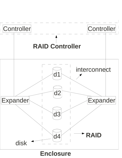
(a) 1 enclosure

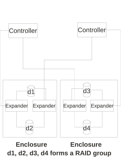
(b) 2 enclosure

Figure 1: 4 disk RAID5 in 1 and 2 enclosures

While the first two redundancy mechanisms clearly increase the reliability of the system, analysis is needed to know when spanning is beneficial.

3 Definitions and Assumptions

Definition 1

[RAID5 Reliability] A RAID5 group experiences “data inaccessibility or data loss” (DIL) if

1. data in any of two disks in the RAID5 group are inaccessible. The data in a disk is said to be inaccessible if some component in its access path fails or the disk itself fails.

2. Or, a data of a disk is inaccessible and an unrecoverable error occurs during rebuild of the data.

We can extend the above definition to RAID6 and other RAID systems by changing the number of inaccessible data disks in the first part of the definition.

3.1 Newer Reliability Measures

Definition 2

[MTTDIL] Mean Time before “any” of the RAID groups experiences “data inaccessibility or data loss” (DIL). This denotes the average time before which at least one user using the system experiences data unavailability.

Note that MTTDIL has lower value than MTTF as inaccessibility of data is also taken into account, not just data loss. It is therefore a composite measure of availability and reliability.

Given the computational flexibility with the use of PRISM toolset [10], it is possible to compute specific reliability measures as needed by the system at hand. Due to lack of space we describe them in Appendix 0.A

We have chosen the “mean” as our reliability measure even though it may not be a good reliability metric [3] as the field data available with us provide only the “mean” values.

3.2 Modelling assumptions

Due to the lack of relevant disk failure parameters in the field data (as needed in detailed disk models such as 5.1), we build our models incrementally and, at each stage, check with field data available for the storage system as a whole.

1. Initially, we assume uncorrelated failures across components. Later, we consider correlated failures for disks in our model and show that the model results match the field data available to us.

2. For a disk, we assume at the start a simple 3-state Markov model (with burn-in rate, pre-burn-in failure rate, post burn-in failure rate [5]) but later consider Weibull models. We assume constant failure rate for all other components as we have access only to MTTF values.

3. We also assume constant repair rate for all the components but this is not necessary.

3.3 Model input parameters

Table 1 shows MTTF values of the components obtained from a few storage vendors. Meanwhile, disk MTTF has been taken from previous literature [7, 4]. We have used Mean Time to Repair (MTTR) of a non-critical component as 30 min based on some inputs from industry.

Components	MTTF value
Disk	33 yr
Controller	604440 hr
Expander	2560000 hr
Enclosure	28400 hr if $\leqslant$ 50% full, else 11100 hr
Interconnect	200000 hr

Table 1: MTTF of components

For all the computational results reported in this paper, we have used a 2.8GHz 8GB RAM machine with 16GB swap space.

4 Modelling RAID5 systems with a simple disk model

In the beginning, we give a brief introduction to other possible modelling aprroaches and compare them with our approach using PRISM. In the later subsections we describe our models using PRISM.

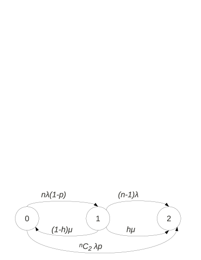
Figure 2: Model of a $n$ disk RAID5 in an enclosure assuming disk correlated failure; State 0: working, 1: one disk fails, 2: data loss, $h$: probability of unrecoverable error during rebuild, $\lambda$: disk failure rate, $\mu$: rebuild rate

4.1 PRISM: Comparison with other approaches

Continuous Time Markov Chains (CTMC) have been used widely to build reliability models of systems. For example, a simple Markov reliability model of RAID5 is given by Rao et al. [7] (see Fig.2 with $p$=0). For more complex configurations or for modelling other components such as enclosures, tool-enabled computational models are critical.

Another approach for evaluating such complex systems is Monte-Carlo simulation techniques where one has to manually find all the system failure cases by keeping a timeline for each of the components. However, writing simulation code for such non-trivial systems is error-prone or the results cannot be validated easily.

Here, we use a model checking tool, PRISM (Probabilistic Symbolic Model Checker) [10], to build and analyze the CTMC models. PRISM has a modular process algebra based language with a probability and reward operator, and it supports quantitative model checking. This is suitable for modelling the reliability of systems as the failure mode of each component can be described in a module separately. Given a PRISM program, PRISM uses matrix computations for exact model checking (by numerical solution technique) of logical formulae (in continuous stochastic logic, CSL), as well as a sampling based simulation approach that is suitable when the state size is very large. We use both approaches according to the size of the model. All our models are reliability models and hence there are no transitions in our models out of the “data inaccessible or loss” state of a specific instance of a RAID system when we calculate MTTDIL.

Our modelling environment in PRISM is much more feasible for modelling large complex storage systems compared to the Monte-Carlo simulation techniques as, in case of PRISM, the tool itself, in effect, does the work of finding all the system failure cases for us, by building a CTMC model of the whole system, from model description written in the PRISM modelling language. Moreover, in case of rare-event failures simulation may take a long time compared to the PRISM model checking (we show such an example in Section 5.1.1).

In the following section, we describe several modelling and state-space reductions techniques for our systems. Section 4.2 presents results of modelling of some small systems mainly using PRISM model checker. Section 4.3 uses PRISM discrete-event simulator to calculate reliability measures for larger systems. Section 4.4 presents the hierarchical decomposition technique to model even larger systems. Section 4.5 presents results of modelling some known field configurations (such as multiple controller pair configurations) along with how they agree with field data.

4.2 PRISM model of small systems

In RAID systems, there are some components connected in series (such as the controller, interconnect and expander in Fig.1(a)). To reduce the state space, we can compose them: if there is a set of components $com_{1}$, $com_{2}$, …., $com_{k}$ in series and if each component has the same repair rate, then we can replace the set by an equivalent component $com$ such that failure rate of $com$ = $\sum_{i=1}^{k}$ $f(i)$, where $f(i)$ is failure rate of the $i$-th component in series and repair rate of $com$ is $\mu$ where $\mu$ is repair rate of each component (Fig.3).

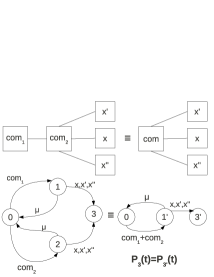
Figure 3: Composing in-series components: $com_{1}$ and $com_{2}$ are in series and can be replaced by series equivalent $com$ as the Markov model at right is equivalent to the model at left. $x$/$x^{\prime}$/$x^{\prime\prime}$ stands for the transitions corresponding to other components i.e. those that are not connected in series with $com_{1}$ and $com_{2}$. State 1’ is the merged equivalent of states 1 and 2. $P_{i}(t)$ is the transient probability of reaching state $i$

			Enclosure MTTF indep. of no. of disks			Enclosure MTTF $\propto$ no. of disks
$m$	Distribution of disks	States	$t$=12	Time(hr)	Model size(GB)	$t$=2	$t$=3	$t$=4
1	$-$	14827521	27697	0.2	0.3	10975	10975	10975
2	(7+1)	20803073	27676	0.5	0.4	10971	10971	10971
	(6+2)	36399361	14004	1	0.7	7911	7911	7911
	(5+3)	35961985	14004	1.1	0.8	5513	7911	7911
	(4+4)	34561793	14004	0.6	0.8	5513	5513	14004
3	(6+1+1)	36115713	27654	1.2	0.7	10967	10967	10967
	(5+2+1)	77596289	13998	4.3	2.1	7909	7909	7909
	(4+3+1)	62729729	13998	3	1.8	5512	7909	13998
	(3+3+2)	114833281	9372	4.6	7.5	3682	9372	9372
	(4+2+2)	96482561	9372	3.6	2.9	6185	6185	9372
4	(5+1+1+1)	28689665	27630	0.5	0.5	10962	10962	10962
	(4+2+1+1)	53671681	13992	1.4	1	7907	7907	13992
	(3+1+2+2)	109296129	9369	4.6	2.1	6183	9369	9369
	(2+2+2+2)	145866497	7043	1.8	8.1	7043	7043	7043
5	(4+1+1+1+1)	42528513	27606	1.8	0.8	10958	10958	27606
	(3+1+2+1+1)	66852353	13986	4	1.5	7904	13986	13986
	(2+2+2+1+1)	100492801	9366	3.6	1.9	9366	9366	9366
6	(3+1+1+1+1+1)	44301697	27581	0.9	0.7	10954	27581	27581
	(2+2+1+1+1+1)	67861761	13979	1	1.0	13979	13979	13979
7	(2+1+1+1+1+1+1)	45208577	27360	1	0.6	27360	27360	27360
8	(1+1+1+1+1+1+1+1)	8649402441	OOM	$-$	$-$	$-$	$-$	$-$

Table 2: MTTDIL (hr) of a 8 disk RAID5; $m$: number of enclosures; $t$ is the threshold number of disks in an enclosure (max 24 disks) after which its MTTF decreases; OOM: Out of Memory Error; indep.: independent; $\propto$: dependent. Note that MTTDIL of 7000 hours is not indicative of unacceptable data loss as it incorporates non-availability due to interconnect failure.

We replace all the final states (corresponding to different types of failures such as those of enclosure, expander or disk) in our model by a single “fail state”. Using these two optimizations, we are able to reduce the model size and execution time significantly (although, execution time still mainly depends on model input parameters).

Table 2 shows MTTDIL of a 8 disk RAID5 with $m$ enclosures ($m\leqslant 8$) calculated in PRISM. The second column denotes the distribution of disks across enclosures. For $m$ enclosures, $(i_{1}+i_{2}+......+i_{m})$ denotes a configuration with $m$ enclosures where enclosure $j$ contains $i_{j}$ number of disks of the RAID group. Table 2 also shows the MTTDIL values assuming variable failure rate for an enclosure i.e.

enclosure MTTF = 28400 hr if no. of disks in it $\leqslant$ $t$

= 11100 hr otherwise

We have generalized the value of $t$ from 2 to 4 (while for field data it is 50% occupancy) to understand its impact. Given $m$ enclosures, each with some capacity $c$, it is not possible to say what the optimal configuration is without detailed modelling.

The important findings from the analysis of PRISM models are:

1. A 10% increase of enclosure MTTF causes MTTDIL to increase by 9.9%. Hence, the enclosure is the main determining component in the reliability of a RAID group.

2. MTTDIL depends on the number of enclosures present in the system and the distribution of disks of a RAID group across enclosures. For example, consider three cases (Table 2) of distribution of disks in 2 enclosures (4+4), 3 enclosures (6+1+1) and 4 enclosures (3+1+2+2). In the first case, if “any” of the enclosures fail “data inaccessibility” occurs while in the second case only failure of enclosure 1 causes “data inaccessibility”. Hence, spanning increases reliability here. In the third case, out of 4 enclosures, failure of 3 enclosures causes “data inaccessibility”. Hence, spanning decreases reliability compared to case 1.

Based on the results of Table 2 we have designed a algorithm for spanning a RAID group across enclosures which is described in detail in Appendix 0.B.

Configs.	MP	SP	Gain	Extra Cost
(1, 2, R1)	28400	23665	1.2	(1, 1, 3)
(2, 2, R1)	6.68E8	3.39E8	1.97	(0, 2, 4)
(2, 2, R1)	6.68E8	603561	1106	(1, 2, 4)
(1, 4, R5)	28245	23552	1.2	(1, 1, 5)
(2, 4, R5)	14157	11801	1.2	(0, 2, 6)
(2, 4, R5)	14157	12036	1.18	(1, 2, 6)
(4, 4, R5)	4629364	281707	16	(0, 4, 8)
(4, 4, R5)	4629364	528003	8.7	(1, 4, 8)

Table 3: Cost-reliability trade-offs: Configs. $(a,b,c)$: $a$: no. of enclosures, $b$: no. of disks, $c$: RAID group type (R1: RAID1, R5: RAID5); MP: multi-pathing and SP: single-pathing; Gain: reliability gain using multi-pathing; Extra cost $(a,b,c)$ due to multi-pathing: $a$: no. of controllers, $b$: no. of expanders, $c$: no. of SAS cables.

Jiang et al. [1] showed that multi-pathing increases storage reliability. Table 3 shows some configurations both with multi-pathing and single-pathing, and the corresponding MTTDIL values. In some cases, multi-pathing increases reliability by a factor of more than 1000 whereas in some other cases it is much lower. Based on such calculations, cost-reliability trade-offs can be attempted. The redundancy of a component is beneficial only if a single failure of some other component does not cause “data inaccessibility” of a whole RAID group.

4.3 Discrete Event Simulation

Table 2 shows (for $m$=8) that it is not possible to model large systems consisting of multiple RAID groups using PRISM model checker (due to state space explosion). To calculate the reliability measures for larger systems we use PRISM discrete-event simulator. This simulator generates a large number of random paths using the PRISM language model description (without explicitly constructing the corresponding Markov Model), evaluates the result of the given properties on each run, and uses this information to generate an approximately correct result. Currently, PRISM simulator has support only for exponential distribution. We use a confidence parameter of 0.01 and “maximum path length” of 1E9 to calculate our reliability measures. PRISM imposes a maximum path length to avoid the need to generate excessively long or infinite paths.

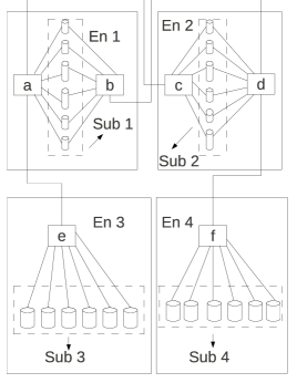
(a) single-pathing in encl. 3/4

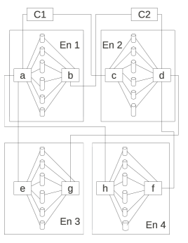
(b) multi-pathing

Figure 4: 4 enclosures 24 disks as 4 RAID5 groups

Fig.4 shows two configurations with multiple RAID groups. Fig.4(a) shows a 4 enclosure 24 disk system with 4 RAID5 groups without redundant paths for disks in enclosures 3 and 4 whereas in Fig.4(b) redundant paths are present for disks in enclosures 3 and 4. Enclosures 3 and 4 are daisy-chained to enclosures 1 and 2 respectively as the controller may not have enough ports to connect all the enclosures present in the system directly. Table 4 gives the MTTDIL for these systems.

It is not possible to simulate larger systems with the required confidence because the time for simulation increases rapidly and we need to decompose our models.

Configs.	Reliability Measures	By Simulation(hr)	Time	By Decomp.(hr)	Err(%)	States	Time
single-pathing	MTTDIL	5940	2.7 hr	5972	0.54	13	137s
multi-pathing	MTTDIL	6968	3.6 hr	7015	0.7	148	137s

Table 4: Results with Simulation and Hierarchical Decomposition for the systems of Fig 4); Err: % diff betw the two results, SMTTDIL: System MTTDIL

4.4 Hierarchical decomposition

From Figs.4(a) and 4(b) we note that the disks and the interconnects that connect the disks of a RAID group to the expanders contribute to the reliability of that particular RAID group. Hence, we can model them separately, i.e. we can divide the whole system into subsystems that can be modelled independently and the submodel results can be used in the higher level model. Each subsystem consists of the disks and the interconnects from expanders to the disks. The subsystems are logically separable rather than physically as each of them is connected to the components shared by all of them (such as a controller). This technique is called “hierarchical decomposition” which is a very general technique to model large systems. Trivedi et al. [6] has applied this technique to model and analyze the reliability of large systems such as telecommunication systems and cloud computing systems. The step of dividing the system into subsystems is called the “decomposition phase” and the step of using the sub-model results into the final model is called the “aggregation phase”.

However, our storage systems are designed with high availability in mind with a multiplicative set of paths and are somewhat different from the systems considered by Trivedi[13] where strong modularity is present with only a few inter-module paths. Each of the modules in the latter can be modelled separately and the outputs of the sub-models can be fixpoint-iterated to get the final result whereas the combinatorial structure of our systems (where each component designed with redundancy in mind has to be connected to all other adjacent non-similar components for high availability) makes it difficult to directly use Trivedi’s technique. Using tool support (such as with PRISM system) is critical to sample the many failure paths to estimate the reliability of such HA systems with good accuracy.

To model a system with multiple RAID groups, we model each of the RAID groups (where a RAID group comprises the disks in it and the interconnects that connect to the disks from expanders) separately and feed the results to the model at a higher level. Hence, we have two levels: RAID group level and system level. If the RAID group itself is too large to model in PRISM, we use hierarchical decomposition to model the RAID group itself, i.e. we model each disk (where a disk also includes its interconnects) separately and feed the results to the model at the RAID group level. Hence, in this case, we have three levels: the disk level, the RAID group level and the system level.

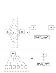
Figure 5: Decomposition phase for the systems of Fig.4

Note that we are using an approximation technique: when we reduce an $n$-state, $m$-transition model (representing a subsystem) to a 2-state, 1-transition model (representing the equivalent component), some errors are introduced. For example, the holding time in the up/down state in the 2-state, 1-transition model is exponentially distributed, while in the original $n$-state $m$-transition model, that may not be true. The necessary conditions for this technique to be exact are:

1. The computed measures are steady-state.

2. The subsystems transformed into “equivalent” model are stochastically independent from other subsystems. If not, the technique can still be used, provided that the dependence can be expressed at some higher level in the hierarchy.

As our reliability measure is “mean” (as opposed to steady state probability measures calculated by Trivedi et al. for his systems), when we use this technique we obtain approximate results. Moreover, when we separately model a subsystem, ignoring the complete system, we lose some failure events. If we do a proper decomposition, these are rare and the accuracy is not affected. Our results show that the accuracy depends on how close the subsystems (independently considered) approach an exponential failure distribution (constant failure rate).

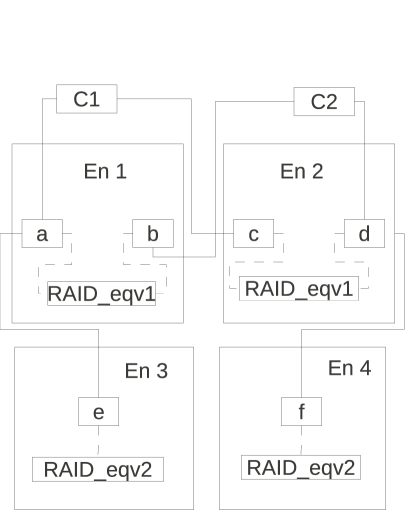
(a) single-pathing

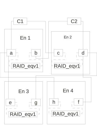
(b) multi-pathing

Figure 6: Aggregation phase for the systems of Fig.4

Fig.4(a) shows 4 subsystems (independently considered) in the system: Sub1, Sub2, Sub3, Sub4. Hence, we have two level hierarchy for the systems of Fig.4. In level 0 (lower level), we model the subsystems (independently considered) and in level 1 (higher level) we model the shared components. Figs.5 and 6 show the decomposition phase and the aggregation phase respectively. We calculate the reliability measures using hierarchical decomposition and the results we obtain is consistent with simulation results (Table 10). We use a shell script to calculate reliability measures for a system using hierarchical decomposition. In the script, lower level model results are calculated first using PRISM and then passed as a input parameter to the next higher level model and so on.

Table 4 shows the results of hierarchical decomposition.

Our results show that the use of hierarchical decomposition is indicated in the following three scenarios:

1. The system is too large to simulate and there is no other option except using hierarchical decomposition.

2. When the system can be simulated but each subsystem considered independently has a constant failure rate (which can be checked using goodness-of-fit tests such as Kolmogorov-Smirnov test).

3. When each subsystem has a small contribution to the reliability of the overall system (which can be checked by sensitivity analysis).

4.5 Modelling of some known field configurations

Tables 5 and 9 shows the MTTF of the components used in some large storage configurations and field MTTDIL value respectively. In these systems, a RAID5 group consists of 6 disks. For the systems with multiple controller pairs, no RAID group is implemented across controller pairs. We model these systems and check whether the model results match the field data.

Components	MTTF (in hr)
Controller	35000
Type1 enclosure(t1)	60000 if $\leqslant$ half-full; else 23000
Type2 enclosure(t2)	50000 when full

Table 5: MTTF of the components for large storage configs.

4.5.1 Modelling single controller-pair systems

1. We simulate the 24 disk system of Table 9 in PRISM simulator with 99% C.I. and $10^{6}$ samples. The time for simulation is 5 hr with MTTDIL = 45859 hr. The subsystem consisting of 24 disks and 48 interconnects contributes very little to the MTTDIL of the whole system; this has been verified using sensitivity analysis. Using hierarchical decomposition, we get MTTDIL as 46098 hr with time for model checking being only 4 min.

2. We use hierarchical decomposition to model the 60 disk system of Table 9 because it is too large to simulate in PRISM. MTTDIL is 20960 hr with time taken for model checking also being 4 min.

4.5.2 Modelling multiple controller pair systems

Fig.7 shows a configuration with multiple controller pairs. We can think of these systems consisting of subsystems each corresponding to one controller pair and not connected to each other. Hence, they are “totally independent” or “physically independent” (they do not share any common components). Here these subsystems are also symmetric. There are various approaches to model such systems:

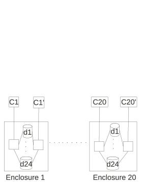
Figure 7: 20 controller pair 20 enclosure 480 disk systems

Hierarchical Decomposition: We model/simulate any one “totally independent subsystem” and do a hypothesis test to check whether a subsystem has a constant failure rate or not. If yes, then MTTDIL of the whole system is = MTTDIL of a subsystem / number of “totally independent” subsystems.

If we can model a “totally independent subsystem” using PRISM model checker or discrete-event simulator, we call this “partial hierarchical decomposition” (P). If a “totally independent subsystem” is too large to model using PRISM simulator we use hierarchical decomposition to model the subsystem itself; we call it “total hierarchical decomposition” (T). We have used both these techniques but due to lack of space we do not present results here.

Simulation of the whole system: When each of the independent subsystems has a non-constant failure rate, then we can simulate the whole system to get a confidence interval for our reliability measure. Let $Y$ be the random variable to denote the time to DIL (data inaccessible or data loss) of the whole system and $X_{1},X_{2},\dots,X_{n}$ be the time to DIL of each of the $n$ independent subsystems. Then $Y=min(X_{1},X_{2},\dots,X_{n})$. To calculate $E[Y]$ we take $N$ observations. In the $i$-th observation we simulate each of the subsystems and get the samples $x_{i1},x_{i2},\dots,x_{in}$ ($x_{ij}$ is the time to DIL of the $j$-th subsystem in $i$-th observation) and calculate $y_{i}=min(x_{i1},x_{i2},\dots,x_{in})$. Estimated $E[Y]$ = $\sum_{i=1}^{N}y_{i}/N$

Discretization process: The ideal approach to model such large systems is to calculate the probability of DIL for a “totally independent subsystem” and calculate the probability of data inaccessibility or loss for the whole system using the formula

$$W(t)=1-(1-F(t))^{n}.$$ (1)

where $W(t)$ is the probability of DIL of the whole system, $F(t)$ is the probability of DIL of a subsystem and $n$ is the number of independent subsystems present in the system. Now,

$$E[X]=\displaystyle\int_{0}^{\infty}(1-W(t))dt=\displaystyle\int_{0}^{\infty}(1-F(t))^{n}dt.$$ (2)

Let $g(t)=(1-F(t))^{n}$. We calculate MTTDIL from this probability values using sampling based techniques as follows: First, we find a maximum range of the random variable $X$ which represents time to DIL. For that we find the value $max$, such that $g(max)<\delta$ where $\delta$ is some error bound, say, 1E-4. Then we divide the range of the random variable ($0$ to $max$) into steps each of size $h$.

$$U =hg(0)+hg(h)+\dots+hg((k-1)h)$$ (3)

$$L =hg(h)+hg(2h)+\dots+hg(kh)$$ (4)

where $U$ and $L$ stands for Upper and Lower Riemann sum respectively. $k$ is the number of steps each of size $h$, so $kh=max$. Clearly,

$$L<E[X]<U$$ (5)

To get a good bound on $E[X]$, our aim is to reduce the difference between $U$ and $L$. Suppose, we want a difference of $\epsilon$ i.e. $U$-$L$ = $\epsilon$. Then

$$U-L=h[g(0)-g(kh)]=h[1-g(kh)]\approx h$$ (6)

assuming $g(kh)=g(max)\approx 0$. Hence, we choose a step size ($h$) of $\epsilon$. The process is shown in Fig.8.

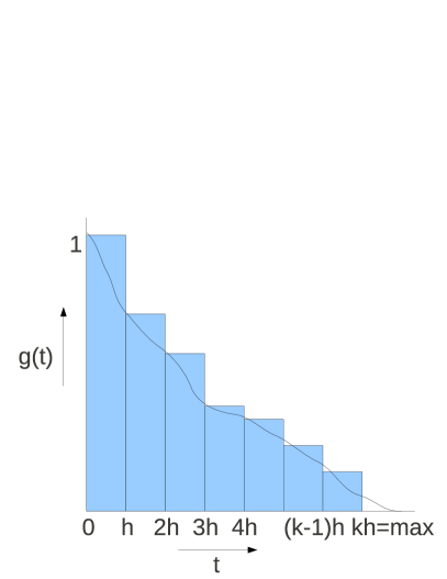
(a) Upper Sum

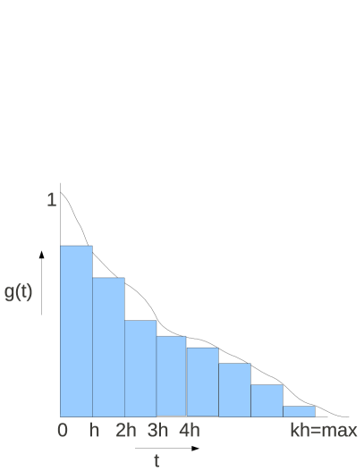
(b) Lower Sum

Figure 8: Discretization approach

For both simulation and discretization approach, we use a shell script to calculate the MTTDIL values. For simulation, the script generates samples (using PRISM simulator) for time to DIL for each “totally independent subsystem” and takes minimum of them, repeats the whole process for the specified number of observations and calculates mean and variance of those minimum values from each observation. In case of discretization approach, the script generates probabilities of DIL for a “totally independent subsystem” at time $t$ where $t$ ranges from 0 to $max$ with a step size of $h$ using PRISM simulator. From these probabilities, we calculate MTTDIL with the sampling technique described above using a C program invoked from the script.

Table 6 under the column labeled “without correlated failure” shows the results after applying these approaches to the systems of Fig.7. We assume $\epsilon$ = 175 hr for the discretization approach.

Comparison between the techniques:

The results using hierarchical decomposition are slightly off from the results using other two approaches. The reason is the constant failure rate assumption of each individual subsystem. We are able to reject the hypothesis in each of the above cases that each individual subsystem has a constant failure rate using Kolmogorov-Smirnov test with 5% level of significance. If each of the individual subsystem has a failure distribution which is far from exponential then it is best to use the simulation approach. The method of calculating mean using discretization approach has an advantage in that the error is bounded (with probability 1) but it has the following disadvantages:

1. Each individual subsystem is modelled using PRISM simulator. Hence, the $F(t)$ result value has some error. When we calculate $W(t)=1-(1-F(t))^{n}$, the error can increase.

2. To get a small difference between $U$ and $L$, we need a small value for step size $h$ i.e. large number of steps. Hence, this procedure can take a long time for small $h$.

4.5.3 Comparison of model results with field data:

Our computed results, however, deviate significantly from the field data. The possible reasons are:

1. Since we do not have field data for disk failure, we may have assumed a simple model for disk failure instead of, for example, Weibull. Disk failure model may affect the result because the number of disks present in the system is much higher than other components.

2. Correlated/burst failure of disks: Many disks in an enclosure may fail within a short span due to high temperature, power supply spikes, vibration etc. thus causing double disk failures almost simultaneously.

To identify the main factors, we consider other disk failure models (such as Weibull disk model or correlated disk failure model) to check whether these models agree with field data.

	without correlated failure				with correlated failure
	480 disk		600 disk		480 disk		600 disk
Methods	MTTDIL (hr)	T	MTTDIL (hr)	T	MTTDIL (hr)	T	MTTDIL (hr)	T
M1	2293	5h	2590	1.11h	1750	25h	1253	3h
M2	2304	4m	2616	4m	1800	10m	1290	10m
M3	2160$\pm$109	29h	2337$\pm$114	36h	1600$\pm$84	38h	1128$\pm$ 48	29h
M4	$L$=2057, $U$=2232	48h	$L$=2308, $U$=2483	48h	$L$=1510, $U$=1685	36h	$L$=1062, $U$=1237	31h

Table 6: Model results for multiple controller pair configs.: M1: Hierarch. Decomp. (P), M2: Hierarch. Decomp. (T), M3: Simulation, M4: Discretization; T: Time. The field data for 480 disk configs. is 1700 hr and for 600 disk configs. is 1200 hr.

5 Detailed model of disk subsystems

5.1 Disk reliability model with Weibull distribution

We use the detailed disk reliability model of Elerath et al. [9]. The model assumptions are as follows: Time to operational failure (TTOp) with a 2-parameter Weibull (shape = 1.12, scale = 461386 hrs); Time to restore (TTR) with a 3-parameter Weibull (shape = 2, scale = 12 hours and offset 6 hours); Time to scrub (TTScr) with a 3-parameter Weibull (shape = 3, scale = 168 hours and offset 6 hours); Time to latent defect (TTLd) with shape = 1 (an exponential distribution) and scale = 9259 hours

Elerath et al. presented a sequential Monte Carlo simulation method using these models to calculate DDF($t$) where DDF($t$) stands for number of double disk failures in time $t$. Elerath also created a simple DDF(t) equation [11] for N+1 RAID systems to calculate expected number of double disk failures. A DDF occurs when any two disks of a RAID5 group experience operational failure or one disk has a latent defect followed by operational failure from another disk. As PRISM does not support anything other than exponential distributions, we approximate Weibull distributions using phase type distributions (sum of exponentials). All of the above Weibull failure/repair models have increasing failure rates. We use the same 3 state model of [5] for each of the Weibull models and find the parameters of the models using the standard technique of moment matching. The pdf (probability density function) of the fail state in the 3-state model is:

$$\dfrac{1}{\sigma+\alpha-\beta}[\beta\sigma e^{-\beta t}+(\alpha-\beta)(\sigma+\alpha)e^{-(\sigma+\alpha)t}]$$

The first three moments of this distribution are:

$$\mu_{1} =\frac{\frac{\sigma}{\beta}+\frac{\alpha-\beta}{\alpha+\sigma}}{\alpha-\beta+\sigma};~{}~{}~{}~{}\mu_{2}=\frac{\beta^{2}+\sigma(2\alpha+\sigma)}{\beta^{2}(\alpha+\sigma)^{2}};~{}~{}~{}~{}\mu_{3}=\frac{2\left(1+\frac{-\alpha^{3}+\beta^{3}}{(\alpha+\sigma)^{3}}\right)}{\beta^{3}}.$$ (7)

Solving these three equations, we obtain $\sigma$, $\alpha$ and $\beta$:

$\sigma=\frac{4\mu_{1}^{3}-6\mu_{1}\mu_{2}+\mu_{3}\pm\sqrt{x}}{y};~{}~{}\alpha=-\frac{2\left(\mu_{1}^{3}-3\mu_{1}\mu_{2}+\mu_{3}\right)}{y};~{}~{}\beta=\frac{2\mu_{1}^{3}-\mu_{3}\mp\sqrt{x}}{y}\ where\\ x=\scriptstyle{-2\mu_{1}^{6}+6\mu_{1}^{4}\mu_{2}-18\mu_{1}^{2}\mu_{2}^{2}+18\mu_{2}^{3}+8\mu_{1}^{3}\mu_{3}-12\mu_{1}\mu_{2}\mu_{3}+\mu_{3}^{2}};~{}~{}y=\scriptstyle{\mu_{1}^{4}+3\mu_{2}^{2}-2\mu_{1}\mu_{3}}\\$

We equate them with the first three moments of Weibull for each of the three cases: TTOp, TTScr, TTR. For TTOp, the solutions turn out to be $\alpha=1.72E-6$ and either $\sigma=2.49E-6$, $\beta=2.88E-6$ or, equivalently $\sigma=1.16E-6$, $\beta=4.21E-6$

5.1.1 Comparison of approx. model with Weibull

To check how well this pdf approximates Weibull distribution, we compare the pdf and hazard functions of approximate and Weibull models (Figures 9). The hazard rate for the approximate model becomes constant after some time. This can be understood by looking into the slope of the hazard rate function for the approximate model :

$$\frac{\sigma(\beta-\alpha)e^{-(\sigma+\alpha+\beta)t}}{(\frac{\sigma}{\sigma+\alpha-\beta}e^{-\beta t}+\frac{\alpha-\beta}{\sigma+\alpha-\beta}e^{-(\alpha+\sigma)t})^{2}}$$

Note that the slope function is a non-negative decreasing function for $\beta>\alpha$. Hence after some time slope becomes zero.

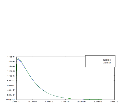
(a) Pdf functions

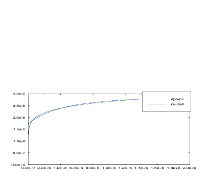
(b) Hazard functions

Figure 9: Approximate vs. Weibull; X axis shows time in hrs

To understand the differences better, we look at the differences between the two CDFs (Approximate minus Weibull). The difference is never more than +0.006 or less than -0.003. Therefore, when using the CDFs to compute probabilities of any interval, the results will never be erroneous by more than 0.006 - (-0.003) = 0.009, less than 1%. The differences in the right tails apparently become zero, indicating the approximation to be very good for right tail probabilities.

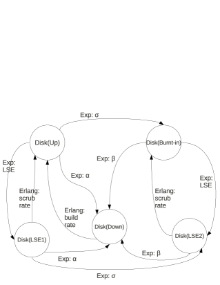
Figure 10: Approx. Disk model based on Gopinath et al. [8]: one difference is that we consider here a more accurate model that has a transition from Disk(LSE1) state to the Disk(LSE2) state with rate $\sigma$ rather than a transition from Disk(LSE1) to Disk(Burnt-in) state.

For TTOP and TTScr, with the same approach, we get complex number for $\sigma$ and $\beta$ and negative value for $\alpha$ for each of the two solutions respectively. Hence, we use other phase type distributions such as Erlang distributions [8]. We use a 3-stage Erlang model. For TTScr $\lambda$ = 0.019228232 and for TTR $\lambda$ = 0.180345653. Using these models for each type of failure/repair we build a detailed disk model (Fig.10).

Comparison of PRISM, Monte Carlo Simulation and DDF(t) equation Results:

We compare the reliability of RAID subsystems using PRISM model, Monte Carlo Simulation and DDF(t) equation (Table 7 and Table 8). We try to keep the variance of both PRISM and Monte Carlo Simulation results same so that we can make a fair comparison. Hence, we set the termination epsilon parameter in case of PRISM and the number of experiments parameter in case of Monte-Carlo simulation accordingly. Results from Table 7 and 8 (under the column with 3-state disk failure model) show that DDF(t) values calculated from PRISM model are similar with that of the MC-Sim and DDF(t) equation. Due to the front-overloading of our approximate pdf (compared to the actual Weibull pdf), the difference between DDF(t) values calculated using PRISM and the other two methods (MC-Sim and DDF(t) equation) is much higher in the beginning.

Time(yr)	pDDF3(t)	pDDF4(t)	sDDF(t)	eqDDF(t)	sDev3(%)	sDev4(%)	eDev3(%)	eDev4(%)
1	7.12	5.59	5.63	5.64	26.5	-0.72	26.24	-0.9
2	14.37	12.2	12.23	12.26	17.5	-0.21	17.21	-0.46
3	21.67	19.26	19.21	19.31	12.8	0.28	12.22	-0.24
4	28.99	26.59	26.43	26.64	9.7	0.59	8.82	-0.20
5	36.35	34.06	33.8	34.21	7.5	0.75	6.26	-0.45
6	43.73	41.6	41.27	41.96	6	0.8	4.22	-0.86
7	51.13	49.17	48.79	49.87	4.8	0.77	2.53	-1.41
8	58.54	56.73	56.36	57.91	3.9	0.66	1.09	-2.09
9	65.96	64.27	63.93	66.08	3.2	0.57	-0.18	-2.73
10	73.39	71.78	71.50	74.35	2.7	0.38	-1.29	-3.46

Table 7: DDF(t) per 1000 RAID groups for 6 disk RAID5 : PRISM Model (PRISM DDF(t)) vs. Simulation (sDDF(t)) vs. DDF(t) equation (eqDDF(t)) result; pDDF_i(t)= DDF calculated in PRISM using $i$-state disk failure model. sDev = Deviation of PRISM results from Simulation results; eDev = Deviation of PRISM results from DDF(t) equation results; Time taken for Model Checking = 37 sec (using 3-state model) and 4.3 min (using 4-state model) while time for Simulation = 8 min; both PRISM and simulation error are 1%;

Time(yr)	PRISM DDF(t)	sDDF(t)	sDev(%)
1	2.26	1.92	17.7
2	4.62	3.84	20.3
3	7.03	6.46	8.8
4	9.51	9.32	2
5	12.04	12.16	-1
6	14.63	14.87	-1.6
7	17.27	18.24	-5
8	19.96	21.52	-7.3
9	22.71	24.56	-7.5
10	25.50	28.16	-9.4

Table 8: DDF(t) per 1000000 RAID groups for 8 disk RAID6 with 3-state model: Time taken for Model Checking = 12.6 min while time for Simulation = 26 hr; PRISM error is 1% and Simulation Error is 4%

It can be noted that the higher deviation between the results of PRISM and simulation due to front overloading of the approximate pdf can be reduced by adding more states in the Markov model. We consider a 4-state model to check how well it approximates Weibull. Note that a 4-state Markov model has 5 model parameters. To estimate them using moment matching will be a very hard problem. Hence we try to estimate the parameters by trial and error method.

Next, we check how this 4-state model performs when modelling disk subsystems. Table 7 (under the column 4-state disk model) shows the DDF(t) values computed using the 4-state model and how it agree with simulation and DDF(t) equation results. Note that in the time period of $t$ = 0 to 10 yr, the deviations are now much less (especially in the initial period), but the hazard rate function starts to flatten much earlier compared to the 3-state model with moment matching. As we calculate mean for the whole system, we use the 3-state model with parameters estimated using moment matching to approximate Weibull model for modelling the whole system.

Apart from the results of Table 7 and 8, our Weibull approximation produces results which are in reasonable agreement with Greenan’s simulation results [12] (details can be found in Appendix 0.C).

5.2 Whole system modelling with detailed model

Assuming the detailed disk model, we can model the large storage systems (Table 9) using hierarchical decomposition. Table 9 shows the results using this detailed disk model of Figure 10. The model results, however, still deviate from the field values, although they are closer to the field data than the results with simple 3 state disk model.

Configs.	Model result(hr)	Field value(hr)
(1, 1, t2, 24)	41396	35000
(1, 1, t1, 60)	18563	11000
(20, 20, t2, 480)	2070	1700
(20, 20, t1, 600)	2253	1200

Table 9: Weibull Model results vs. field value for the large storage configurations. Configs. $(a,b,c,d)$ $a$: number of controller-pairs, $b$: number of enclosures, $c$: type of an enclosure, $d$: number of disks

Hence, we postulate correlated failure as a possible reason for the difference between model results and real system field results. Garth et al. [4] has found existence of strong correlation in disk failures. The study by Jiang et al. [1] also show the existence of correlated failure for disks. They show that RAID group spanned across multiple enclosures exhibit lower correlated failure. The study also shows that the amount of correlation depends on the particular enclosure model. We show that our correlated failure model is consistent with these findings.

5.3 Modelling correlated failure for disks

The key point in modelling correlated failures for disks is that failure events are independent of each other rather than individual disks failing independent of each other. Each failure event may involve multiple disks. Let $p$ be the probability that when a disk fails another disk also fails simultaneously. The value of $p$ depends on the source of correlation (for example, the enclosure).

Fig.2 shows the CTMC model for a RAID5 group consisting of $n$ disks in an enclosure.

We use the “synchronized action” language construct in PRISM to build the model in PRISM: such an action can be used to force two or more modules to make transitions simultaneously with a rate that is product of two rates. For our models, we use one action as the “active action” that actually defines the rate for the synchronized transition and the other one as the passive action with rate as 1.

We model the storage configurations (Table 9) using the revised model and compare them with field data.

5.3.1 Validation

As we do not have any information on $p$ for our systems, we assume a particular disk failure model (i.e. 3-state model or Weibull model), estimate $p$ for each type of enclosure from the field data of 1 enclosure configurations and then use that $p$ to check whether the model results match field value for the multiple controller pair configurations.

The model results are given in Table 6 under the column with the heading “with correlated failure”; these agree with field data quite well.

Modelling the large storage configurations assuming Weibull model along with correlated failure for disks takes around 1.5 hr.

6 Conclusions

We have presented several approaches for reliability modelling of RAID storage systems starting from 4 to 600 disks. Using these models we are able to perform sensitivity analysis, make cost-reliability trade-offs and choose better reliability configurations. To the best of our knowledge, there has been no comparable work in the open literature.

Appendix 0.A Other reliability measures

Generally, a RAID5 group consists of 6-8 disks because a larger number of disks increase the chance of latent sector error during reorganization. Hence one RAID5 group may not be sufficient to store large amounts of data. For systems with multiple RAID groups accessed by multiple users we can define reliability metrics such as the following:

Definition 3

[$k$%System MTTDIL+R(-R)] Mean time before which $k$% of “all” the RAID groups experience “data inaccessibility or data loss” even with (without) repair. With k=50, this is system “half-time” when repair is (is not) possible from the “data inaccessible” state.

In a multiple RAID system, the first measure (MTTDIL) is not sufficiently informative as a sysadm may be interested in knowing how many RAID groups are available for allocation to different users when some RAID groups are undergoing repair (either connectivity or rebuild). With the new measures, a sysadm will be able to select repair rates and disk replacement rates to ensure satisfactory allocations of RAID groups (for example, in a “cloud” setting). Consider also two users A and B where the disks for A are in very highly unreliable enclosures while those for B are not. Although the MTTDIL of the system is very low, B experiences good reliability (as the RAID groups used by B experience high MTTDIL). The $k$%System MTTDIL-R metrics can reflect this information because it consider failures from “data inaccessible or data loss” state and hence not much affected by a single weak link in the system. Therefore it can represent the reliability of a system much better.

For example, for the systems of Figure 4 we claculate the 50% and 100% reliability metrics as shown in the following table.

Configs.	Reliability Measures	By Simulation(hr)	Time	By Decomp.(hr)	Err(%)	States	Time
single-pathing	MTTDIL	5940	2.7 hr	5972	0.54	13	137s
	100%SMTTDIL-R	37027	8 min	35671	-3.6	2340	.31s
	50%SMTTDIL-R	10155	24 min	9048	-11	150	.3
	100%SMTTDIL+R	2146215	7.1 hr	2143599	0.12	2670	138s
	50%SMTTDIL+R	13975	5 hr	14032	.4	150	137s
multi-pathing	MTTDIL	6968	3.6 hr	7015	0.7	148	137s
	100%SMTTDIL-R	37168	10 min	36461	-2	33495	3s
	50%SMTTDIL-R	14169	34 min	13171	-7	5072	0.4s
	100%SMTTDIL+R	2578533	10 hr	2581352	0.1	33495	160s
	50%SMTTDIL+R	593232	9.9 hr	597274	.7	5072	138s

Table 10: Results with Simulation and Hierarchical Decomposition for the systems of Fig 4); Err: % diff betw the two results, SMTTDIL: System MTTDIL

From the table, it is clear that the metric 50%SMTTDIL+R expresses the advantage of using multi-pathing which other metrics do not.Also, repair has a significant impact on 50%SMTTDIL+R.

From the results of Table 10 With multi-pathing, we get 17% higher MTTDIL and 20% higher System MTTDIL+R (100%) compared to single-pathing at the cost of 14 SAS cables and 2 expanders. In this system, if we replace 6 disk RAID5 with 24 disk RAID10 in each enclosure then with multi-pathing we get 7% higher MTTDIL and 2% higher System MTTDIL+R (100%) at the cost of 50 SAS cables and 2 expanders. Such calculations are important for cost-reliability trade-offs. In the first case multi-pathing seems to be a good option while in the second case it is not. The reason is that, in the latter case, the enclosure is less reliable (full enclosure MTTF = 11100 hr) and RAID10 is more reliable than RAID5.

For the 100%System MTTDIL+R and 50% System MTTDIL+R (in case of multi-pathing), the contribution of subsystems (i.e. interconnect and disk subsystem) is very high; this can be verified by sensitivity analysis. Computationally, each of the subsystems considered in isolation has a failure rate that is very close to constant failure rate; we could not therefore reject the hypothesis that each of the subsystems has a constant failure rate at even 20% level of significance in the Kolmogorov-Smirnov test. For other reliability metrics, the contribution of subsystems (i.e. interconnect and disk subsystem) is much less; the enclosure having an exponential failure distribution is the main contributor; this has been verified by sensitivity analysis. Hence the results of hierarchical decomposition and simulation is almost same for all the reliability measures we have calculated.

Appendix 0.B How to span a RAID group across enclosures ?

0.B.1 Without correlated failure

How should a storage system designer distribute the disks of a RAID group across enclosures to get the maximum reliability? For a $n$ disk RAID5 group, it is best to distribute it across $n$ enclosures (because no single enclosure failure causes data inaccessibility of the whole RAID5 group) but this may not be cost effective or possible. Hence, one has to choose the best configuration among the sub-optimal solutions rather than having the luxury of choosing the optimal solutions. Here we present a greedy algorithm to find the optimum configuration for any $f$ tolerant RAID group given $n$ disks and $m$ enclosures (Algorithm 1).

Algorithm 1 Greedy algorithm for spanning

while $n>0$ do

     if $n\leqslant mf$ then

         Place $f$ disks at a time in each of the empty enclosures until number of disks left ($l$) is less than $f$. Place these $l$ disks in the next enclosure.

         break;

     else

         $C\leftarrow$ highest available capacity amongst remaining enclosures

         $d\leftarrow min(C,n)$

         Fill the chosen enclosure with $d$ disks

         $n\leftarrow n-d$

         $m\leftarrow m-1$

     end if

end while

In Fig.11(a), we need to design a 14 disk RAID5 group using 2 enclosures where the failure rate of an enclosure is as stated in Table 1.

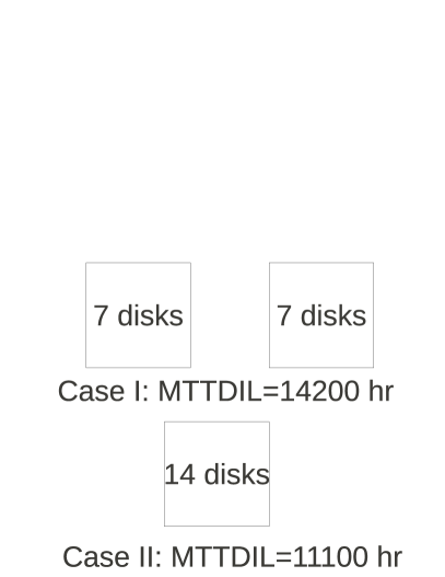
(a) spanning increases reliability

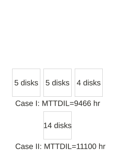
(b) spanning decreases reliability

Figure 11: Enclosure failure rate $\propto$ no. of disks inside it

Using algorithm 1, the optimal configuration is to put all the disks in one enclosure. We obtain MTTDIL = 11100 hr. Algorithm 1 assumes that all the enclosures have the same MTTF. However, an enclosure is a shared component whose failure rate depends on the number of disks present in it. If we span the disks across 2 enclosures such that each of them contains less than or equal to 12 disks, we get MTTDIL = 14200 hr. In Fig.11(b), spanning a RAID group across 3 enclosures decreases reliability; here we used the PRISM simulator for the computation.

0.B.2 with correlated failure

Spanning a RAID group across enclosures Suppose, a $n$ disk RAID5 group is formed inside an enclosure. Then the rate at which data loss occurs due to correlated failure is ${}^{n}\mathrm{C}_{2}\lambda p$. Now, if the $n$ disks are distributed across $m$ enclosures (where $m>1$ and, for simplicity, $n$ is a multiple of $m$ with each enclosure containing $n/m$ disks), then the rate at which data loss occurs due to correlated failure is $m[^{(n/m)}\mathrm{C}_{2}]\lambda p=\frac{(n((n/m)-1))\lambda p}{2}$ that is less than ${}^{n}\mathrm{C}_{2}\lambda p$ for $m>1$. Hence with respect to “only” correlated failures, spanning is a good option.

But, whether spanning will increase the chance of overall “data inaccessibility or data loss” will depend on enclosure failure rate also (Fig.12). In Fig.12, for $p$ = 0.4, spanning is beneficial when enclosure MTTF is 60000 hr. but not useful if enclosure MTTF is 28400 hr. Similarly, for a given enclosure MTTF, say 60000 hr, spanning is beneficial when $p$ = 0.4 but not useful when $p$ = 0.2.

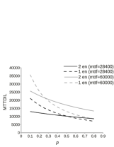
Figure 12: MTTDIL (hr) for a RAID group of 8 disks using correlated disk failure model. en: enclosure

Appendix 0.C Memorylessness assumption of Markov Model and our solution:

Kevin Greenan has raised several questions regarding suitability of Markov models as a tool to measure storage reliability [12], as neither component wear-out nor rebuild progress can be modelled using a system level Markov model due to its memoryless property. The reason is that the notion of “absolute” time is present in a system level Markov model whereas “relative time” for each component is needed and simulation is the only solution.

We propose a solution for this problem by considering failure and repair modes of each disk separately rather than considering a system level Markov model. Moreover, when we approximate Weibull repair and Weibull failure by summation of exponentials (i.e. by adding multiple states and transitions corresponding to a single failure/repair transition) then these states keep information regarding repair progress and age of a component respectively. Hence, our disk subsystem models using detailed disk models reduce the chance of loss of information due to memorylessness property significantly.

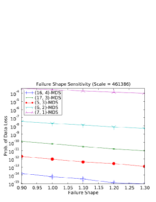
(a) Simulation results [12]

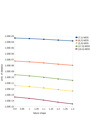
(b) PRISM results

Figure 13: Comparison of PRISM results with Greenan’s simulation results

To prove our claim, we modelled some disk subsystem configurations from Greenan’s thesis [12] in PRISM and compared them with the Greenan’s simulation results (Fig. 13). We see that PRISM results are in reasonable agreement with his simulation results.

References

- [1] Weihang Jiang, Chongfeng Hu, Yuanyuan Zhou, Arkady Kanevsky, “Are Disks the Dominant Contributor for Storage Failures? A Comprehensive Study of Storage Subsystem Failure Characteristics,” FAST, 2008.
- [2] Daniel Ford, François Labelle, Florentina I. Popovici, Murray Stokely, Van-Anh Truong, Luiz Barroso, Carrie Grimes, Sean Quinlan, “Availability in Globally Distributed Storage Systems,” OSDI, 2010.
- [3] Kevin M. Greenan, James S. Plank, Jay J. Wylie, “Mean time to meaningless: MTTDIL, Markov models, and storage system reliability,” HOTSTORAGE, 2010.
- [4] Bianca Schroeder, Garth A. Gibson: Disk Failures in the Real World, “What Does an MTTF of 1, 000, 000 Hours Mean to You,” FAST, 2007.
- [5] Qin Xin, Thomas J. E. Schwarz, Ethan L. Miller, “Disk infant mortality in large storage systems,” MASCOTS, 2005.
- [6] M. Lanus, Liang Yin, Kishor S. Trivedi, “Hierarchical composition and aggregation of state-based availability and performability models,” IEEE Transactions on Reliability, Pages 44-52, 2003.
- [7] K. K. Rao, James Lee Hafner, Richard A. Golding, “Reliability for Networked Storage Nodes,” DSN, 2006: 237-248.
- [8] K. Gopinath, Jon Elerath, Darrell Long, “Reliability Modelling of Disk Subsystems with Probabilistic Model Checking,” Technical Report UCSC-SSRC, May 2009.
- [9] Jon G. Elerath, Michael Pecht, “Enhanced Reliability Modeling of RAID Storage Systems,” DSN 2007.
- [10] www.prismmodelchecker.org
- [11] Jon G. Elerath. “A Simple Equation for Estimating Reliability of an N+1 Redundant Array of Independent Disks (RAID),” DSN’09
- [12] Kevin Greenan’s Phd thesis http://www.kaymgee.com/Kevin_Greenan/Publications.html
- [13] Rahul Ghosh, Kishor S. Trivedi, Vijay K. Naiky, and Dong Seong Kim, “End-to-End Performability Analysis for Infrastructure-as-a-Service Cloud: An Interacting Stochastic Models Approach”