Differential Hanbury-Brown-Twiss for an exact hydrodynamic model with rotation

Abstract

We study an exact rotating and expanding solution of the fluid dynamical model of heavy ion reactions, that take into account the rate of slowing down of the rotation due to the longitudinal and transverse expansion of the system. The parameters of the model are set on the basis of realistic 3+1D fluid dynamical calculation at TeV energies, where the rotation is enhanced by the build up of the Kelvin Helmholtz Instability in the flow.

I Introduction

In peripheral heavy ion collisions the participant system has large angular momentum. In hydrodynamical model calculations it has been shown that this shear leads to a significant vorticity CMW13 ; Vov14 . When Quark-Gluon Plasma (QGP) is formed with low viscosity CKM ; KSS ; NNG , new phenomena may occur like rotation hydro1 , or turbulence, which shows up in form of a starting Kelvin-Helmholtz Instability (KHI) hydro2 ; YH ; WNC13 . It was also shown CF that in peripheral collisions even if the shear flow is neglected and the same boost invariant longitudinal velocity is assumed at all transverse points, in the Color Glas Condensate (CGC) model initial transverse flow develops and it contributes to angular momentum in the same direction as the angular momentum arising from the target and projectile motion in the participant system.

Rotation in heavy ion collision has only recently been considered, our aim is to detect it using two particle correlation.

The Differential Hanbury Brown and Twiss (DHBT) method has been introduced earlier in DCF . Previously the method has been applied to a high resolution Particle in Cell Relativistic (PICR) fluid dynamical model DCF2 . Here we will look at how the DHBT can be used for the exact hydro model CsoN14 ; ReHM . Rotation in exact models have been investigated as well in HNX .

We look at the values from the exact hydro model and determine the effect rotation has on the correlation functions (CF) for detectors at different positions.

II Correlation function for exact hydro model.

The two particle correlation function for this model is found with the same method used in DCF where the source function is

$$S(x,k)=\frac{n(x)k^{\mu}\sigma_{\mu}}{C_{n}}\exp\left[-\frac{k^{\mu}u_{\mu}}{T(x)}\right]\ ,$$ (1)

where $C_{n}$ is a constant, $k^{\mu}$ is the average 4 vector momentum of two pions, $k=(p_{1}+p_{2})/2$ and the momentum difference is $q=(p_{2}-p_{1})$, $u_{\mu}$ is the 4-vector velocity of the source, $\sigma_{\mu}$ is the normal of the freeze out hypersurface and $T(x)$ is the temperature distribution. The density for the exact hydro model ReHM is given by

$$N(r_{\rho},r_{y})=N_{B}\frac{C_{n}}{V}\exp(-r^{2}_{\rho}/2R^{2})\exp(-r^{2}_{y}/2Y^{2})$$ (2)

or using the scaling variables in the out ($\rho,\ R$), side ($\varphi,\ \Theta$), long ($y,\ Y$) directions

$$N(s_{\rho},s_{y})=N_{B}\frac{C_{n}}{V}\exp(-s_{\rho}/2)\exp(-s_{y}/2),$$ (3)

where $s_{\rho}=r^{2}_{\rho}/R^{2}$ and $s_{y}=r^{2}_{y}/Y^{2}$.

We use the finite size cylindrical shape source as described in eq. (10) of ReHM

$$\int_{0}^{\infty}\!\!\!\int_{-\infty}^{\infty}\int_{0}^{2\pi}\!\!\!r_{\rho}dr_{\rho}dr_{y}d\varphi=R^{2}Y\!\!\int_{0}^{1}\!\!\int_{0}^{1}\!\!\int_{0}^{2\pi}\frac{ds_{y}ds_{\rho}d\varphi}{\sqrt{s_{y}}},$$ (4)

and the integral $J(k,q)$ for this model will be

$$\begin{split}J(k,q)\propto&\int_{0}^{1}\int_{0}^{1}\int_{0}^{2\pi}w_{s}\gamma_{s}\left(k_{0}+\mbox{\boldmath$k$}\cdot\mbox{\boldmath$v_{s}$}\right)\times\\ &\exp\left[-\frac{\gamma_{s}}{T_{s}}((k_{0}+q_{0}/2)-(\mbox{\boldmath$k$}+\mbox{\boldmath$q$}/2)\cdot\mbox{\boldmath$v_{s}$})\right]\times\\ &\exp(i\mbox{\boldmath$q$}\cdot\mbox{\boldmath$x$})e^{-s_{\rho}/2}e^{-s_{y}/2}\frac{ds_{y}ds_{\rho}d\varphi}{\sqrt{(s_{y})}}\ ,\end{split}$$ (5)

where $k_{0}=\sqrt{\frac{2m_{\pi}}{\hbar c}+k^{2}}$ and $q_{0}=\dfrac{\mbox{\boldmath$k$}\cdot\mbox{\boldmath$q$}}{k_{0}}$, $w_{s}$ is a weight function, $w_{s}\propto k^{\mu}\sigma_{\mu}$, and the temperature profile is flat with a value of 250 MeV.

We have the single particle distribution integral

$$\begin{split}&\int d^{4}xS(x,k)\propto\int w_{s}\gamma_{s}\left(k_{0}+\mbox{\boldmath$k$}\cdot\mbox{\boldmath$v_{s}$}\right)\times\\ &\exp\left[-\frac{\gamma_{s}}{T_{s}}(k_{0}-\mbox{\boldmath$k$}\cdot\mbox{\boldmath$v_{s}$})\right]e^{-s_{\rho}/2}e^{-s_{y}/2}\frac{ds_{y}ds_{\rho}d\varphi}{\sqrt{(s_{y})}}\ ,\end{split}$$ (6)

and the correlation function is given by DCF

$$C(k,q)=1+\frac{Re[J(k,q)J(k,-q)]}{\left|\int d^{4}xS(x,k)\right|^{2}}$$ (7)

so the constants outside the integrals will cancel.

The velocity consists of a radial expansion in the out direction, an angular velocity, where the rotation is in the reaction plane and also an axis-directed expansion in the side direction. The velocity in the out ($\rho$), side ($\varphi$), long-direction ($y$) is then

$$\mbox{\boldmath$v$}_{s}=\left(\dot{R}\sqrt{s_{\rho}},R\omega\sqrt{s_{\rho}},\dot{Y}\sqrt{s_{y}}\right)\ ,$$ (8)

or in the $x,\ y,\ z$ directions where $x$ is the direction of the impact parameter, $y$ is the longitudinal (rotation) axis and $z$ is the (beam) collision axis.

$$\begin{split}&\mbox{\boldmath$v$}_{s}=\left(\dot{R}\sqrt{s_{\rho}}\ \sin(\varphi)+R\omega\sqrt{s_{\rho}}\ \cos(\varphi),\right.\\ &\left.\dot{Y}\sqrt{s_{y}},\dot{R}\sqrt{s_{\rho}}\ \cos(\varphi)-R\omega\sqrt{s_{\rho}}\ \sin(\varphi)\right)\ .\end{split}$$ (9)

The average transverse radius is $R=\sqrt{XZ}$, and we use this value when the exact model is studied. Using the values from Table 1 we show the correlation function as function of $q=q_{out}$ in Figures 1 $a$ and $b$ for two different configurations.

​​​​​​ ​​​​​​

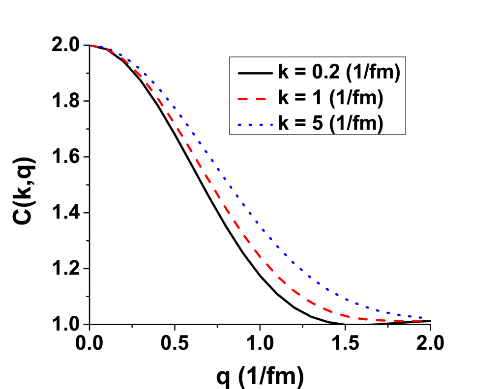
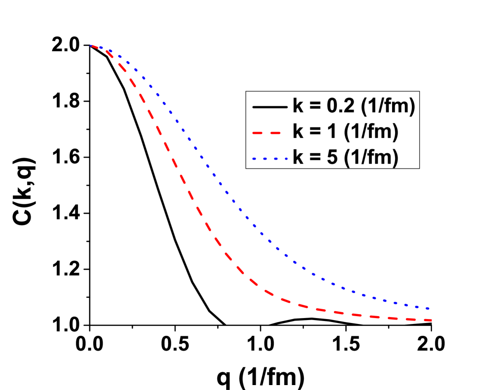
Figure 1: (color online) Correlation Function $C(k,q_{out})$ for the exact hydro model as function of $q=q_{out}$, with
(a) R = 2.500 fm, $\dot{R}$ = 0.250 c, Y = 4.000 fm, $\dot{Y}$ = 0.300 fm, $\omega$ = 0.150 c/fm,at t = 0.0 fm/c. (left figure)
(b) R = 3.970 fm, $\dot{R}$ = 0.646 c, Y = 5.258 fm, $\dot{Y}$ = 0.503 fm, $\omega$ = 0.059 c/fm, at t = 3.0 fm/c. (middle figure)
(c) R = 7.629 fm, $\dot{R}$ = 0.779 c, Y = 8.049 fm, $\dot{Y}$ = 0.591 fm, $\omega$ = 0.016 c/fm, at t = 8.0 fm/c. (right figure)
The solid black line is for $k=0.2\,fm^{-1}$, the dashed red line is for $k=1\,fm^{-1}$ and the dotted blue line is for $k=5\,fm^{-1}$.

As the system size increases with time we get a narrower distribution in $q_{out}$ for the correlation function. We also notice a wider distribution for increasing values of $k$.

III Results - Differential HBT for exact hydro model.

Let us now ”Event by Event” evaluate two correlation functions at two different k-vectors in the plane of rotation. The differential correlation function DCF is obtained by taking the difference between the correlation functions with e.g. at detector positions $\mbox{\boldmath$k$}^{+}=(a,0,b)k$ and subtracting the CF for a detector at $\mbox{\boldmath$k$}^{-}=(a,0,-b)k$ $(a^{2}+b^{2}=1)$ in $x,y,z$ coordinates,

$$\Delta C(k,q)\equiv C(\mbox{\boldmath$k$}^{+},\mbox{\boldmath$q$})-C(\mbox{\boldmath$k$}^{-},\mbox{\boldmath$q$})\ .$$ (10)

The integrals for this model cannot be given in analytic form, so the CF and DCF need to be integrated numerically. The momentum difference vector $q$ may point in different directions, and it is usual to use the $q_{out},\ q_{long},\ q_{side}$ system of directions. In the present work we show the $q_{out}$ dependence of the Correlation functions only, where $\mbox{\boldmath$k$}\parallel\mbox{\boldmath$q$}_{out}$.

Detectors

As we can see from eq. (8) the rotation leads to an asymmetry, both the $\rho$ and $\varphi$ components of the velocity $\mbox{\boldmath$v$}_{s}$ depend linearly on $\sqrt{s_{\rho}}$, thus the flow velocities of the system at a given FO time have a velocity profile $v_{s}^{(\varphi)}={\rm const.}v_{s}^{(\rho)}$. The corresponding momentum of the fluid motion has approximately the same characteristics, and this is indicated by the red full line in Fig. 2. This characteristic flow velocity distribution determines the final momentum distribution of the emitted particles where the contribution of a fluid element at a radial coordinate $s_{\rho}$ leads to a tangential momentum distribution centered around $v_{s}^{(\varphi)}=R\omega\sqrt{s_{\rho}}$. The resulting momentum distribution of the emitted particles from different radii are sketched in Fig. 2.

${}^{|}_{|}$ $t$	$Y$	$\dot{Y}$	$\omega$	$R$	$\dot{R}$	$\varphi$
(fm/c)	(fm)	(c)	(c/fm)	(fm)	(c)	(Rad)
0.	4.000	0.300	0.150	2.500	0.250	0.000
3.	5.258	0.503	0.059	3.970	0.646	0.307
8.	8.049	0.591	0.016	7.629	0.779	0.467

Table 1: Time dependence of some characteristic parameters of the fluid dynamical calculation presented in ref. ReHM . R is the average transverse radius, Y is the longitudinal length of the participant system, $\varphi$ is the angle of the rotation of the interior region of the system, around the $y$-axis, measured from the horizontal, beam ($z$) direction in the reaction, $[x,z]$ plane, $\dot{R},\ \dot{Y}$ are the speeds of expansion in transverse and longitudinal directions, and $\omega$ is the angular velocity of the internal region of the matter during the collision.

Although our spatial source configuration is azimuthally symmetric, our phase-space configuration is not, because of the given direction of the rotation. As eq. (5) shows the CF depends on $\mbox{\boldmath$q$}\cdot\mbox{\boldmath$v$}_{s}$ and $\mbox{\boldmath$q$}\cdot\mbox{\boldmath$x$}$, thus reversing the direction of either $q$ or $\mbox{\boldmath$v$}_{s}$ will change the CF! For vanishing rotation the CF would be the same for different azimuthal angles (e.g. $d_{z}=\pm b$) if the spatial source is azimuthally symmetric. If there is no expansion the rotation does not change the CF integrals either.

We use a detector placed at $(x,y,z)=(0.935,0,0.353)$, so that $\mbox{\boldmath$k$}=(0.935,0,0.353)k$ and $\mbox{\boldmath$q$}=\mbox{\boldmath$q$}_{out}=(0.935,0,0.353)q_{out}$, so that both $k$ and $q$ are parallel, are in the reaction plane and are orthogonal to the rotation axis, $y$.

If we look at the azimuthal integrals for $\mbox{\boldmath$k$}\cdot\mbox{\boldmath$v$}_{s}$ for the detectors at $\mbox{\boldmath$k$}=\left(ak,0,\pm bk\right)$ in eqs. (5,6), we have the integrals below, which will have a non-zero difference for $a\neq b$, $\dot{R}\neq 0$ and $\omega\neq 0$, both for $k$ and $\mbox{\boldmath$q$}_{out}$:

$$\int_{0}^{2\pi}\!\!\!\exp\left(k\sqrt{s_{\rho}}\ \left(a[\dot{R}\sin(\varphi)+R\omega\cos(\varphi)]\right.\right.$$

$$\left.\left.+c[\dot{R}\cos(\varphi)-R\omega\sin(\varphi)]\right)\right)d\varphi$$

$$\neq\int_{0}^{2\pi}\!\!\!\exp\left(k\sqrt{s_{\rho}}\ \left(a[\dot{R}\sin(\varphi)+R\omega\cos(\varphi)]\right.\right.$$

$$\left.\left.-c[\dot{R}\cos(\varphi)-R\omega\sin(\varphi)]\right)\right)d\varphi\ \ .$$ (11)

This is so because, although the spatial distribution does not depend on $\varphi$, the momentum space distribution depends on $v_{\varphi}$.

In the case of a realistic dynamical configuration, especially in the initial configuration, the local rotation velocity component from the shear flow is maximal at higher distances in the $\pm x$ directions and pointing towards the $\pm z$ direction.

For different detector positions we would expect different values of the correlation function, and ideally we would place them along or near the direction of highest speed in the side direction which would usually be in the beam direction.

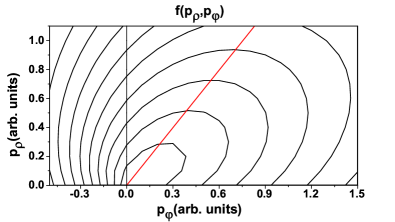
Figure 2: (color online) The schematic phase space distribution of the rotating and expanding source in the momentum space. The momentum of the expansion increases with the radius just as the momentum arising from the rotation. So, higher radial flow momenta correspond to higher rotation momenta also, as given by eq.(8) and indicated by the red line. At constant $p_{\rho}$ the distribution peaks at the momentum $p_{\phi}$ indicated by the red line; the Jüttner distribution, eq.(8), is not symmetric, it is elongated towards higher momenta, see Sec. 2.4.2 of LPS . The resulting thermally smeared distribution is indicated by the contour lines.

In the exact model discussed here we can see that at small values of $k$ there is little to no difference in the DCF, but the difference will increase for higher values. As the system grows in size the distribution becomes more narrow for the CF and the DCF will become smaller for larger values of the relative momentum q.

For the initial time, t=0, the DCF is small and positive, Figure 3 $a$, but for the later times the amplitude is larger and negative. Comparing Figures 3 $b$ and $c$ we see that as expected the peaks of the DCF are more to the left for larger size because $R\sim 1/q$ at half width of the correlation function. We also see that the amplitude for DCF for Figures 3 $b$ and $c$ are about the same. As the system continues to increase in size we would see a decrease in the amplitude because of the lower $\omega$ value. For higher values of the temperature we get a smaller amplitude in the DCF, or for smaller values of the temperature we get a higher amplitude. At late times, $t=8$ fm/c and larger size, the CF is much more narrow as shown in Figure 1 $c$. Notice that at low wave numbers, $k$ the CF has several zero points. This is also reflected in the DCF at the same $k$ value, see Figure 3 $c$.

​​​​​​ ​​​​​​

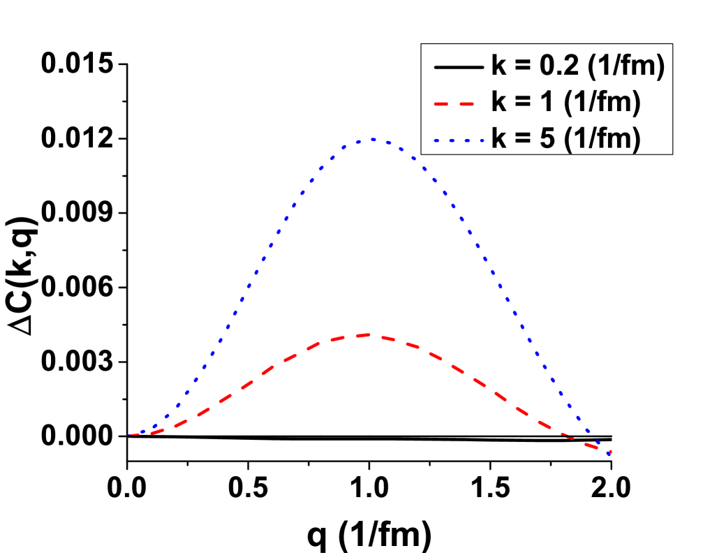
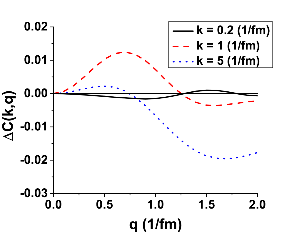
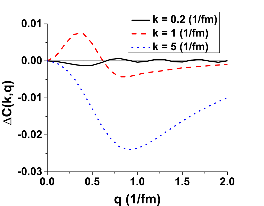
Figure 3: (color online) Differential Correlation Function for the exact hydro model as function of $q=q_{out}$, with
(a) R = 2.500 fm, $\dot{R}$ = 0.250 c, Y = 4.000 fm, $\dot{Y}$ = 0.300 fm, $\omega$ = 0.150 c/fm at t = 0.0 fm/c. (left figure)
(b) R = 3.970 fm, $\dot{R}$ = 0.646 c, Y = 5.258 fm, $\dot{Y}$ = 0.503 fm, $\omega$ = 0.059 c/fm at t = 3.0 fm/c. (middle figure)
(c) R = 7.629 fm, $\dot{R}$ = 0.779 c, Y = 8.049 fm, $\dot{Y}$ = 0.591 fm, $\omega$ = 0.016 c/fm at t = 8.0 fm/c. (right figure)
Where the solid black line is for $k=0.2\,fm^{-1}$, the dashed red line is for $k=1\,fm^{-1}$ and the dotted blue line is for $k=5\,fm^{-1}$. In (a) the solid black line is close to the axis.

The DCF is dependent on the positions of the detectors as demonstrated in Figure 3. This dependence can be used to maximize the amplitude of DCF in a given configuration, based on previous theoretical estimates. Measuring a single CF at different azimuthal angles in the plane of rotation does provide the same $C(k,q)$-s as our model is azimuthally symmetric! Thus, the difference is caused by the measuring two CFs in one event with the same source function homogeneity area, but two different k-vectors at different azimuths with respect to the source area. This is also indicated by eq. (27) of DCF , where the $\epsilon$ sinh$\left(\frac{2\mbox{\boldmath$k$}\cdot\mbox{\boldmath$u_{s}$}}{T_{s}}\right)$ factor appears, which leads to the sensitivity on vector $k$.

IV Conclusion

The model calculations show that the Differential HBT method can give a measure of rotation in this exact hydro model. The differential correlation function is dependent on shape, temperature, radial velocity and angular velocity. Also the detector position is important.

If we eliminate rotation or the radial expansion the DCF vanishes in the model. It also indicates that using the estimated small rotation velocities, $\omega=0.01-0.15$ c/fm, we get a DCF value approaching 2-3 %.

References

- (1) L.P. Csernai, V. K. Magas, D. J. Wang, Phys. Rev. C 87, 034906 (2013).
- (2) V. Vovchenko, D. Anchishkin, and L.P. Csernai, Phys. Rev. C 90, 044907 (2014).
- (3) L.P. Csernai, J. I. Kapusta, L. D. McLerran, Phys. Rev. Lett. 97, 152303 (2006).
- (4) P.K. Kovtun, D.T. Son and A.O. Starinets, Phys. Rev. Lett. 94, 111601 (2005).
- (5) J. Noronha-Hostler, J. Noronha, and C. Greiner, Phys. Rev. Lett. 103, 172302 (2009).
- (6) L.P. Csernai, V.K. Magas, H. Stöcker, and D.D. Strottman, Phys. Rev. C 84, 024914 (2011).
- (7) L.P. Csernai, D.D. Strottman and Cs. Anderlik, Phys. Rev. C 85, 054901 (2012).
- (8) A. Yamamoto, and Y. Hirono, Phys. Rev. Lett. 111, 081601 (2013).
- (9) D.J. Wang, Z. Néda, and L.P. Csernai, Phys. Rev. C 87, 024908 (2013).
- (10) G.-Y. Chen and R.J. Fries, J. Phys. Conf. Ser. 535, 012014 (2014).
- (11) L.P. Csernai and S. Velle, Int. J. Mod. Phys. E 23, 1450043 (2014).
- (12) L.P. Csernai, S. Velle, and D. J. Wang, Phys. Rev. C 89, 034916 (2014).
- (13) T. Csörgő and M.I. Nagy, Phys. Rev. C 89, 044901 (2014).
- (14) L. P. Csernai, D. J. Wang, and T. Csörgő, Phys. Rev. C 90, 024901 (2014).
- (15) Y. Hatta, J. Noronha, and B.-W. Xiao, Phys. Rev. D 89, 051702 (2014); and Phys. Rev. D 89, 114011 (2014).
- (16) L.P. Csernai: Introduction to Relativistic Heavy Ion Collisions (Wiley, 1994).