Abstract

The process of diffusion is the most elementary stochastic transport process. Brownian motion, the representative model of diffusion, played a important role in the advancement of scientific fields such as physics, chemistry, biology and finance. However, in recent decades, non-diffusive transport processes with non-Brownian statistics were observed experimentally in a multitude of scientific fields. Examples include human travel[Brockmann2006, Song2010], in-cell dynamics[Caspi2000], the motion of bright points on the solar surface[Lawrence2001], the transport of charge carriers in amorphous semiconductors[Scher1975], the propagation of contaminants in groundwater[Kirchner2000], the search patterns of foraging animals[Ayala-Orozco2004] and the transport of energetic particles in turbulent plasmas[Perri2009, Bovet2014nf, Bovet2014prl, effenberger2014parameter, Bovet2015, Bovet2015phd]. These examples showed that the assumptions of the classical diffusion paradigm[Einstein1905, Smoluchowski1906, Langevin1908], assuming an underlying uncorrelated (Markovian), Gaussian stochastic process, need to be relaxed to describe transport processes exhibiting a non-local character and exhibiting long-range correlations.

This article does not aim at presenting a complete review of non-diffusive transport, but rather an introduction for readers not familiar with the topic. For more in depth reviews, we recommend the references[Samorodnitsky1994, Metzler2000, Metzler2004, Mainardi2001]. First, we recall the basics of the classical diffusion model and then we present two approaches of possible generalizations of this model: the continuous time random walk (CTRW) and the fractional Lévy motion (fLm).

1 Classical diffusion and the random walk model

The model of the random walk was first developed by Einstein[Einstein1905] in 1905 and, independently, by Smoluchowski[Smoluchowski1906] in 1906, to explain the observation made by a Scottish botanist, Robert Brown (1773-1858), of the random motion of pollen particles in suspension on water. The term Brownian motion has been coined in honors of Brown to designate the random walk. In 1913, in his book Les Atomes[Perrin1913], Perrin verified the results of Einstein and Smoluchowski by measuring with a microscope the displacement of small particles in suspension in a liquid. Figure 1 reproduces some of his observations. Using Einstein’s theory, he was able to measure the Avogadro Number[Philibert2005]. This remarkable success bore the definite proof of the existence of the atom which awarded Perrin the Nobel Prize for physics in 1926.

Einstein’s model of the random walk assumes that each individual particle motion is independent of the other’s and that the displacements of the same particle at different times are also independent, provided that the interval separating the different times is not too small. Next, he introduces a time interval, $\tau$, very small compared to the observation time but sufficiently large so that the motions between two consecutive time intervals $\tau$ can be considered as independent. In a one-dimensional (1D) model, considering $n$ particles, during the time interval $\tau$, each particle position along the $x$-axis will increase by a value $\Delta$, different for each particle. The probability distribution function (PDF) of the step sizes $\varphi(\Delta)$ is defined by the following relation: the number $\operatorname{d}n$ of particle experiencing a displacement lying between $\Delta$ and $\Delta+\operatorname{d}\Delta$ is given by

$$\operatorname{d}n=n\varphi(\Delta)\operatorname{d}\Delta\mbox{.}$$ (1)

The step size probability satisfies the relation $\varphi(\Delta)=\varphi(-\Delta)$ and differs from zero only for very small values of $\Delta$.

Let $f(x,t)$ be the distribution of particles. Using eq. 1, the number of particles at time $t+\tau$ found between $x$ and $x+\operatorname{d}x$ is written

$$f(x,t+\tau)\operatorname{d}x=\operatorname{d}x\int_{-\infty}^{+\infty}f(x+\Delta,t)\varphi(\Delta)\operatorname{d}\Delta\mbox{.}$$ (2)

Since $\tau$ is very small, we can write

$$f(x,t+\tau)=f(x,t)+\tau\frac{\text{\rotatebox[origin={t}]{13.0}{\scalebox{0.95}[1.0]{$\partial$}}}f}{\text{\rotatebox[origin={t}]{13.0}{\scalebox{0.95}[1.0]{$\partial$}}}t},$$ (3)

and by expanding $f(x+\Delta,t)$ in powers of $\Delta$, we find

$$f(x+\Delta,t)=f(x,t)+\Delta\frac{\text{\rotatebox[origin={t}]{13.0}{\scalebox{0.95}[1.0]{$\partial$}}}f(x,t)}{\text{\rotatebox[origin={t}]{13.0}{\scalebox{0.95}[1.0]{$\partial$}}}x}+\frac{\Delta^{2}}{2}\frac{\text{\rotatebox[origin={t}]{13.0}{\scalebox{0.95}[1.0]{$\partial$}}}^{2}f(x,t)}{\text{\rotatebox[origin={t}]{13.0}{\scalebox{0.95}[1.0]{$\partial$}}}^{2}x}+O(\Delta^{3})\mbox{.}$$ (4)

We note that, after the assumption of independent time steps and symmetrically distributed step sizes, we assume here that $\tau$ and $\Delta$ cannot take large values in order to perform the two previous expansions. This is, as we will see below, a fundamental restriction of the diffusive model which gives it its local character in time and space.

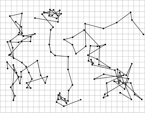
Figure 1: Example of trajectories of small particles (radius of $0.53\text{\,}\mathrm{\SIUnitSymbolMicro}\mathrm{m}$) in suspension in a fluid measured by Jean Perrin[Mandelbrot1983fractal]. The successive positions are marked every $30\text{\,}\mathrm{s}$ and joined by straight lines to guide the eye. The grid size is $3.2\text{\,}\mathrm{\SIUnitSymbolMicro}\mathrm{m}$.

Since only very small values contribute to it, the expansion can be performed under the integral. We find

$$f(x,t)+\tau\frac{\text{\rotatebox[origin={t}]{13.0}{\scalebox{0.95}[1.0]{$\partial$}}}f}{\text{\rotatebox[origin={t}]{13.0}{\scalebox{0.95}[1.0]{$\partial$}}}t}=f\int_{-\infty}^{+\infty}\varphi(\Delta)\operatorname{d}\Delta+\frac{\text{\rotatebox[origin={t}]{13.0}{\scalebox{0.95}[1.0]{$\partial$}}}f}{\text{\rotatebox[origin={t}]{13.0}{\scalebox{0.95}[1.0]{$\partial$}}}x}\int_{-\infty}^{+\infty}\Delta\varphi(\Delta)\operatorname{d}\Delta+\frac{\text{\rotatebox[origin={t}]{13.0}{\scalebox{0.95}[1.0]{$\partial$}}}^{2}f}{\text{\rotatebox[origin={t}]{13.0}{\scalebox{0.95}[1.0]{$\partial$}}}^{2}x}\int_{-\infty}^{+\infty}\frac{\Delta^{2}}{2}\varphi(\Delta)\operatorname{d}\Delta+O(\Delta^{3})\mbox{.}$$ (5)

All the terms with odd powers of $\Delta$ vanish due to the fact that $\varphi(\Delta)=\varphi(-\Delta)$. Taking into account the fact that $\int_{-\infty}^{+\infty}\varphi(\Delta)\operatorname{d}\Delta=1$, defining the variance of the step sizes

$$\left<\Delta^{2}\right>=\int_{-\infty}^{+\infty}\Delta^{2}\varphi(\Delta)\operatorname{d}\Delta$$ (6)

and retaining the terms up to $O(\Delta^{3})$, we find the well-known diffusion equation

$$\frac{\text{\rotatebox[origin={t}]{13.0}{\scalebox{0.95}[1.0]{$\partial$}}}f}{\text{\rotatebox[origin={t}]{13.0}{\scalebox{0.95}[1.0]{$\partial$}}}t}=D\frac{\text{\rotatebox[origin={t}]{13.0}{\scalebox{0.95}[1.0]{$\partial$}}}^{2}f}{\text{\rotatebox[origin={t}]{13.0}{\scalebox{0.95}[1.0]{$\partial$}}}^{2}x}\mbox{,}$$ (7)

where $D=\frac{\left<\Delta^{2}\right>}{2\tau}$ is the diffusion coefficient. The equation of diffusion had already been discovered experimentally by Fick in 1855, but Einstein was the first to derive it from this physical and atomistic model.

Let us now find the fundamental solution, $G(x,t)$, of eq. 7, i.e. the solution of the equation with initial condition $G(x,t=0)=\delta(x)$. This solution is also called the Green function or the propagator of the equation. Its convolution with an arbitrary initial condition $f_{0}(x)$ provides the evolution of the initial condition at all times $t>0$

$$f(x,t)=\left(G\ast f_{0}\right)(x,t)=\int_{-\infty}^{+\infty}G(x-x^{\prime},t)f_{0}(x^{\prime})\operatorname{d}x^{\prime}\mbox{.}$$ (8)

As we will see later, it is interesting to take the Fourier transform in space of eq. 7

$$\frac{\text{\rotatebox[origin={t}]{13.0}{\scalebox{0.95}[1.0]{$\partial$}}}\hat{G}(k,t)}{\text{\rotatebox[origin={t}]{13.0}{\scalebox{0.95}[1.0]{$\partial$}}}t}=-k^{2}D\hat{G}(k,t)\mbox{,}$$ (9)

where

$$\hat{G}(k,t)=\int_{-\infty}^{+\infty}e^{-ikx}G(x,t)\operatorname{d}x\mbox{.}$$ (10)

The solution of eq. 9 is

$$\hat{G}(k,t)=Ce^{-k^{2}Dt}\mbox{.}$$ (11)

As $\hat{G}(k,0)=\int_{-\infty}^{+\infty}e^{-ikx}\delta(x)\operatorname{d}x=1$, we find that $C=1$.

We find the solution by taking the inverse Fourier transform of the previous expression

$$G(x,t)=\frac{1}{2\pi}\int_{-\infty}^{+\infty}e^{-k^{2}Dt+ikx}\operatorname{d}k=\frac{1}{2\pi}\int_{-\infty}^{+\infty}e^{-\left(Dt\left(k-\frac{ix}{2Dt}\right)^{2}+\frac{x^{2}}{4Dt}\right)}\operatorname{d}k\mbox{.}$$ (12)

After a little effort, one finds that the solution is the Gaussian, or normal, distribution

$$G(x,t)=\frac{1}{\sqrt{4\pi Dt}}e^{-\frac{x^{2}}{4Dt}}\mbox{,}$$ (13)

with a variance, or mean-squared displacement, given by

$$\left<x^{2}\right>=2Dt.$$ (14)

The linear time dependence of the mean-square displacement of diffusive processes is a fundamental results of the random walk model.

The fact that the distribution of positions of the random walkers is a Gaussian distribution arises naturally from the central limit theorem (CLT). Indeed, the position of each particle is a sum of independent and identically distributed steps having the same mean and the same variance. Each step being independent, the diffusive process is also memory-less, i.e. Markovian.

2 Non-diffusive transport

Since its discovery, the model of diffusion and Brownian motion plays a crucial role not only in physics but also in biology, chemistry, sociology, economics and finance. However, numerous examples of transport show a deviation from the diffusive paradigm given by eq. (14). Non-diffusive transport is in fact ubiquitous in nature. Examples ranges from the dispersal of bank notes[Brockmann2006], the motion of particles inside living cells[Caspi2000] or the foraging movements of spider monkeys[Ayala-Orozco2004]. In plasma physics, examples are also multiple. The acceleration of electrons and ions by interplanetary shocks in the solar wind[Perri2009], ion transport across the magnetopause[Greco2003], the motion of magnetic bright points on the solar surface[Lawrence2001] or the transport of tracer particles in 3D pressure-gradient driven turbulence[Carreras2001] are evidences indicating the presence of non-diffusive transport in magnetized plasmas.

Non-diffusive transport is characterized by a mean-squared displacement (variance of displacement) of an ensemble of individuals that does not necessarily scale linearly with time

$$\left\langle\left(\bm{r}(t)-\left<\bm{r}(t)\right>\right)^{2}\right\rangle\propto t^{\gamma},$$ (15)

where $\bm{r}(t)$ represents the positions of individuals and $\gamma$ is called the transport exponent. When $\gamma>1$ or $\gamma<1$, the transport is called superdiffusive or subdiffusive, respectively. For the special case of classical diffusion, $\gamma=1$ in accordance with eq. (14). When $\gamma=2$, the transport is ballistic. Non-diffusive transport is at the heart of many complex systems, such as turbulence, where well-defined scale-lengths or time-scales do not exist, and thus transport cannot be modeled as a classical diffusive process. In these systems, the transport is characterized by the presence of long-term memory and/or non-Gaussian (heavy-tailed) PDFs. Mandelbrot coined the terms Noah effect and Joseph effect[Mandelbrot1968noahjosef], as a reference to the natural events experienced by these biblical figures, to describe those two effects in the context of hydrology. The great flood experienced by Noah and the seven years of abundance followed by seven years of famine experienced by Joseph are well known examples that reflects that extreme events with low probability and cycles or trend do, in fact, occur in nature.

In order to account for these effects, the hypotheses of the CLT need to be loosen. By removing the restriction on the finiteness of the variance of the random variables (here, the step sizes), we allow large fluctuations in the random walk. The limiting distributions in this case are given by the generalized central limit theorem, due to the work of Lévy, Khintchine, Gnedenko and Kolmogorov[Khintchine1936, Bouchaud1990, Samorodnitsky1994] in the 1930. They are called $\alpha$-stable distributions and are presented in appendix LABEL:sec:stable_dist. They are characterized by their index of stability, $\alpha\in(0,2]$, and include the Gaussian distribution as a special case, for $\alpha=2$. When $\alpha<2$, they have algebraically decaying heavy tails with exponent $-(1+\alpha)$, and infinite variance. For this reason, they are particularly interesting to model stochastic processes with high variability, such as solar flare intermittency[Scafetta2003]. By removing the hypothesis on the independence of the steps of the CLT, we allow for long-time correlations in the Brownian motion.

In the next section, we introduce the model of the continuous time random walk (CTRW)which is a generalization of the random walk. We give two notable examples of this model, the Lévy-flight and the Lévy-walk. Finally, we introduce an other model of non-diffusive transport which is based on the Langevin equation of motion and includes long-range temporal correlations, the fractional Brownian motion (fBm)and its generalization to a non-Gaussian, heavy-tailed process, the fractional Lévy motion (fLm).

2.1 Continuous time random walk

The model of the CTRW was first developed in 1965 by Montroll and Weiss to describe the mobility of charges in amorphous semiconductors[Montroll1965]. It has since then found a wide range of applications in physics, chemistry, biology, etc. The CTRW supposes that a particle, also called random walker, makes successive jumps interrupted by rests. The step sizes and the waiting times are drawn from a PDF, called the jump PDF, $\psi(x,t)$. Various choices of the form of $\psi(x,t)$ lead to different situations. For example, if the step sizes and the waiting times are independent random variables, the CTRW is decoupled and the jump PDF can be written as $\psi(x,t)=\lambda(x)w(t)$, where $\lambda(x)$ and $w(t)$ are the step size PDF and the waiting time PDF, respectively. In the case of a coupled jump PDF, a jump of a certain length involves a certain duration. This is, for example, the case of the Lévy-walk.

The CTRW can be described by the equation[Klafter1987]

$$\eta(x,t)=\int_{-\infty}^{+\infty}\operatorname{d}x^{\prime}\int_{0}^{+\infty}\operatorname{d}t^{\prime}\eta(x^{\prime},t^{\prime})\psi(x^{\prime}-x,t-t^{\prime})+\delta(x)\delta(t),$$ (16)

which links the PDF $\eta(x,t)$ of arriving at position $x$ at time $t$ with the PDF $\eta(x^{\prime},t^{\prime})$ of being arrived at position $x^{\prime}$ at time $t^{\prime}$ with a delta Dirac initial condition.

For the decoupled case, the PDF of the density of walkers is therefore given by

$$n(x,t)=\int_{0}^{t}\operatorname{d}t^{\prime}\eta(x,t^{\prime})\Psi(t-t^{\prime})\operatorname{d}t^{\prime},$$ (17)

where $\Psi(t)=1-\int_{0}^{t}w(t^{\prime})\operatorname{d}t^{\prime}$ is the probability for a walker of making no jumps between the time interval $(0,t)$.

By taking the space Fourier transform and time Laplace transform of eq. (17), one finds the Montroll-Weiss equation

$$\hat{n}(k,s)=\frac{1-\hat{w}(s)}{s(1-\hat{w}(s)\hat{\lambda}(k))}.$$ (18)

Starting from this equation, the fluid limit, meaning that all details of the CTRW that are irrelevant at very large temporal and spatial scales are neglected, is usually sought to find a equation describing the temporal evolution of the density of random walker.

For example, classical diffusion is found by taking a Gaussian distribution of step sizes and a Poissonian wating time PDF. In fact, the fluid limit is always found to be the classical diffusion, as long as the characteristic waiting time

$$\tau=\int_{0}^{+\infty}tw(t)\operatorname{d}t$$ (19)

and the variance of step sizes

$$\Delta^{2}=\int_{-\infty}^{+\infty}x^{2}\lambda(x)\operatorname{d}x$$ (20)

are finite[Metzler2000]. In this case the diffusion coefficient is given by $D=\Delta^{2}/\tau$.

To describe non-diffusive transport, $\lambda$ and $w$ have to be chosen such that $\tau$ or $\Delta^{2}$, or both, diverge. A natural choice is to draw both functions in the family of stable distributions (with certain restrictions) since they are the limit of sums of random variables[Sanchez2005]. The non-Gaussian property will arise from a divergent $\Delta^{2}$ and the non-Markovianity from a divergent $\tau$. In the case where both characteristic scales diverge, we can choose a strictly symmetric stable distribution with characteristic exponent $\alpha<2$ for the step sizes distribution and a one-sided stable distribution with characteristic exponent $\beta<1$ for the waiting time distribution (see appendix LABEL:sec:stable_dist):

$$\hat{\lambda}(k)=e^{-\sigma^{\alpha}|k|^{\alpha}}\simeq 1-\sigma^{\alpha}|k|^{\alpha}\text{\,\,\, for \,\,\,}k\rightarrow 0\text{\,\,\, with \,\,\,}\alpha<2$$ (21)

and

$$\hat{w}(s)=e^{-\mu^{\beta}s^{\beta}}\simeq 1-\mu^{\beta}s^{\beta}\text{\,\,\, for \,\,\,}s\rightarrow 0\text{\,\,\, with \,\,\,}\beta<1,$$ (22)

with the following asymptotic behavior

$$\lambda(x)\sim x^{-(\alpha+1)},\text{\,\,\, when \,\,\,}|x|\rightarrow\infty$$ (23)

and

$$w(t)\sim x^{-(\beta+1)},\text{\,\,\, when \,\,\,}t\rightarrow\infty.$$ (24)

Using those expression in eq. (18) and keeping terms up to first order, one finds

$$\hat{n}(k,s)=\frac{s^{\beta-1}}{s^{\beta}+\frac{\sigma^{\alpha}}{\mu^{\beta}}|k|^{\alpha}},$$ (25)

which can be rearranged as

$$s^{\beta}\hat{n}(k,s)-s^{\beta-1}=-\frac{\sigma^{\alpha}}{\mu^{\beta}}|k|^{\alpha}\hat{n}(k,s).$$ (26)

If $\alpha=2$ and $\beta=1$, one recognizes the Laplace transform of the first order time derivative of $\hat{n}(k,t)$ on the left hand side (lhs) and the Fourier transform of the second order space derivative of $\hat{n}(x,s)$ on the right hand side (rhs). Therefore, in this case, we recover the classical diffusion equation (eq. (7)) with $D=\sigma^{2}/\mu$.

In the case were $\alpha<2$ and $\beta<1$, the lhs and rhs correspond to generalizations of the differential operator to fractional orders (see appendix LABEL:sec:fract_ope)

$$\frac{\text{\rotatebox[origin={t}]{13.0}{\scalebox{0.95}[1.0]{$\partial$}}}^{\beta}}{\text{\rotatebox[origin={t}]{13.0}{\scalebox{0.95}[1.0]{$\partial$}}}t^{\beta}}n(x,t)=D_{\alpha,\beta}\frac{\text{\rotatebox[origin={t}]{13.0}{\scalebox{0.95}[1.0]{$\partial$}}}^{\alpha}}{\text{\rotatebox[origin={t}]{13.0}{\scalebox{0.95}[1.0]{$\partial$}}}|x|^{\alpha}}n(x,t),$$ (27)

where $D_{\alpha,\beta}=\sigma^{\alpha}/\mu^{\beta}\,[$\mathrm{m}^{\alpha}\mathrm{/}\mathrm{s}^{\beta}$]$ is a generalized diffusion coefficient. This equation is called the space and time fractional diffusion equation and describes the time evolution of the fluid limit of a CTRW with long-term memory (non-Markovian) and long-range spatial correlations (non-Gaussian). When $\alpha\rightarrow 2$ and $\beta\rightarrow 1$, the classical diffusion equation (eq. (7)) is recovered. We call $\alpha$ the spatial transport exponent and $\beta$ the temporal transport exponent. The time derivative operator is the Caputo fractional derivative and the space derivative is the Riesz fractional derivative (appendix LABEL:sec:fract_ope).

By using the scaling properties of the Fourier and Laplace transform

$$\mathcal{F}[f(ax)]=|a|^{-1}\hat{f}(k/a)\text{\,\,\, and \,\,\,}\mathcal{L}[f(bu)]=b^{-1}\hat{f}(s/b),\,\,\,b>0,$$ (28)

on eq. (25), the following scaling property of the propagator of eq. (27) is inferred

$$G_{\alpha,\beta}(x,t)=t^{-H}K_{\alpha,\beta}\left(\frac{x}{t^{H}}\right),$$ (29)

where $\lx@glossaries@gls@link{main}{hurst}{\leavevmode H}=\beta/\alpha$ is the self-similarity index also called Hurst exponent[Saenko2009], $K_{\alpha,\beta}$ is called the reduced Green function and $\frac{x}{t^{H}}$ is the similarity variable[Mainardi2001]. This scaling implies that the stochastic process associated with the propagator is self-similar with index $\lx@glossaries@gls@link{main}{hurst}{\leavevmode H}=\beta/\alpha$ (or $H$-self similar). Indeed, if we rescale the time by a factor $\lambda>0$, we find

$$G_{\alpha,\beta}(x,\lambda t)=\lambda^{-H}t^{-H}K_{\alpha,\beta}\left(\frac{x}{t^{H}\lambda^{H}}\right)\propto G_{\alpha,\beta}(x\lambda^{-H},t),$$ (30)

implying that the motion is invariant under the following transformation

$$(x,t)\mapsto(\lambda^{H}x,\lambda t).$$ (31)

The self-similarity of the process leads then to the following scaling of the moments of the distribution with time

$$\left<|x|^{s}\right>\propto t^{sH}.$$ (32)

Indeed, if we assume $\left<|x|^{s}\right>\propto t^{K}$, we have

$$\left<|\lambda^{H}x|^{s}\right>\propto(\lambda t)^{K}\,\,\,\,\Rightarrow\,\,\,\lambda^{sH}\left<|x|^{s}\right>\propto\lambda^{K}t^{K}\,\,\,\,\Rightarrow\,\,\,K=sH.$$ (33)

By identifying eq. (15) with eq. (32) we see that $\gamma=2H$. The transport is therefore superdiffusive if $2\beta>\alpha$ and subdiffusive if $2\beta<\alpha$. For the special case $2\beta=\alpha,\beta\neq 1,\alpha\neq 2$ the transport is called quasidiffusive[Brockmann2006] and exhibits the same scaling as the classical diffusion despite the crucial difference of a non-Gaussian PDF and non-Markovian time increments. We would like to point out that only verifying the time dependence of the variance of displacements is not sufficient to conclude that a transport process is diffusive. Whenever possible, the temporal evolution of higher moments, or of the full distribution, should be examined to determine the presence of non-Gaussian features. Evaluating moments of the distribution can be delicate since the integrals that define them do not always converge. For example, the $s$-order moments of a $\alpha$-stable distributions converges only for $s<\alpha$[Samorodnitsky1994]. However, in practice, the temporal scaling can be recovered by taking “truncated” moments or by computing moments of fractional order smaller than $\alpha$[Metzler2000].

2.1.1 Lévy flight

The Lévy flight is a particular case of the CTRW with a finite characteristic waiting time, $\tau<\infty$, but step size distribution given by a symmetric stable distribution with diverging variance, $\Delta^{2}\rightarrow\infty$. The trajectories of Lévy flights have been shown to model the foraging motions of many living organisms[Ayala-Orozco2004, Reynolds2009]. Mandelbrot also used this model to simulate the fractal galaxy distribution in the Universe[Mandelbrot1983fractal]. In fact, a fractal dimension $D=\alpha$ can be assigned to the trajectories. An example of a Lévy flight trajectory is shown in fig. 2.

Figure 2: Example of a Lévy flight trajectory with $\alpha=1.5$. Contrary to the Brownian motion (fig. 1), arbitrary long steps can arise, on all scale length, leading to the clustering nature of the Lévy flight.

The Lévy flight can be modeled by taking a Poissonian distribution for the waiting time PDF $w(t)=\tau^{-1}e^{-t/\tau}$, with Laplace transform $\hat{w}(s)=(1+s\tau)^{-1}\simeq 1-\tau s$, for $s\rightarrow 0$. Using this in eq. (18), we find

$$\hat{G}_{\alpha}(k,s)=\frac{1}{s+\frac{\sigma^{\alpha}}{\tau}|k|^{\alpha}},$$ (34)

which, upon Fourier-Laplace inversion, shows that the propagator of the Lévy flight is a symmetric stable distribution

$${G}(x,t)=t^{-H}L_{\alpha,\sigma}\left(\frac{x}{t^{H}}\right),$$ (35)

with a self-similar index $\lx@glossaries@gls@link{main}{hurst}{\leavevmode H}=1/\alpha$. Rearranging the terms of eq. (34) and Fourier-Laplace inverting it, we find the space fractional diffusion equation

$$\frac{\text{\rotatebox[origin={t}]{13.0}{\scalebox{0.95}[1.0]{$\partial$}}}}{\text{\rotatebox[origin={t}]{13.0}{\scalebox{0.95}[1.0]{$\partial$}}}t}n(x,t)=D_{\alpha}\frac{\text{\rotatebox[origin={t}]{13.0}{\scalebox{0.95}[1.0]{$\partial$}}}^{\alpha}}{\text{\rotatebox[origin={t}]{13.0}{\scalebox{0.95}[1.0]{$\partial$}}}|x|^{\alpha}}n(x,t)$$ (36)

describing the Lévy flight.

The Lévy flight results in a superdiffusive process (with the exception of the case $\alpha=2$) with a diverging mean-square displacement $\left<x^{2}\right>\rightarrow\infty$ for $\alpha<2$.

The presence of arbitrary long jumps without any restriction on the step duration leads to rather unphysical situations[Metzler2000, Metzler2004]. One way of solving this is introduced in the Lévy walk model, which is often more appropriate to describe physical systems.

2.1.2 Lévy walk

Similarly to the Lévy flight, the Lévy walk model maintains a diverging variance of distribution of step sizes. However, a coupling between the step sizes and the step duration is included in the jump pdf such that[Klafter1987, Gustafson2012levy]

$$\psi(x,t)=\lambda(x)\delta(|x|-vt^{\nu}),$$ (37)

where $\lambda(x)\rightarrow|x|^{-\mu}$ as $|x|\rightarrow\infty$ and $v$ is a generalized velocity which penalizes long jumps such that the variance is finite[Metzler2004]. Depending on the values of the two exponent $\mu$ and $\nu$ the transport can be either superdiffusive or subdiffusive. Due to the coupled form of the jump pdf, the derivation of a transport equation describing the evolution of the PDF has only been achieved recently in the case $\nu=1$, by using a fractional version of the material derivative[Sokolov2003].

2.2 Langevin approach

A microscopic description of Brownian motion equivalent to the one of Einstein presented in sec. 1 was introduced by Langevin in 1908[Langevin1908] An uncorrelated Gaussian noise, representing the random force due to the interaction with the fluid molecules, is used in the equation of motion of a test particle. The equation of motion becomes a stochastic equation, whose average motion shows the same diffusive scaling. Fractional Brownian motion (fBm) introduces long-range temporal dependence in the Gaussian noise, which can lead to a non-linear scaling of the positional variance. On the other hand, non-Gaussian statistics can be introduced by choosing a non-Gaussian noise. For example, stable Lévy motion[Samorodnitsky1994] replaces the Gaussian noise with a random noise distributed according to a Lévy stable distribution with heavy-tails (appendix LABEL:sec:stable_dist).

The classical Langevin equation is written[Langevin1908]

$$m\ddot{x}(t)=-m\gamma\dot{x}(t)+\xi(t),$$ (38)

where $m$ is the mass of the test particle, $\gamma$ is the friction coefficient and $\xi(t)$ is the random force due to the random collisions with the surrounding particles. In the case of the Brownian motion, $\xi(t)$ is a a white noise, i.e. a Gaussian noise with an infinitely short correlation time: $\left<\xi(t_{1})\xi(t_{2})\right>=C\delta(t_{1}-t_{2})$, where $C$ is a constant. In eq. 38, the forces acting on the particle are separated in two groups, the macroscopic, slowly varying ones, represented by the dissipative force $-m\gamma v$, and the microscopic, rapidly varying ones, represented by the fluctuating force $\xi(t)$.

If the time scale of the particle motion is comparable to the time scale of the collisions, the assumption of a white noise and a constant friction have to be abandoned. This leads to the generalized Langevin equation (GLE)[Kubo1966]

$$\ddot{x}(t)=-\int_{0}^{t}\beta(t-t^{\prime})\dot{x}(t^{\prime})\operatorname{d}t^{\prime}+\xi(t),$$ (39)

where $m=1$ is used for simplicity. Here, $\beta(t)$ is the memory kernel and $\xi(t)$ is the random force which is zero-centered and stationary, i.e. $\left<\xi(t_{1})\xi(t_{2})\right>=C(|t_{1}-t_{2}|)=C(\tau)$. The fluctuation-dissipation theorem[Nyquist1928fluctdiss, Callen1951fluctdiss, Kubo1966, Porr1996] states that the dissipation is the macroscopic manifestation of the disordering effect of the fluctuations and relates the correlation function of the random forces $C(t)$ with $\beta(t)$ by

$$k_{B}T\beta(t)=C(t).$$ (40)

Assuming $x(0)=0$, $v(0)=v_{0}$ and Laplace transforming eq. (39), we find

$$\hat{x}(s)=\frac{v_{0}+\hat{\beta}(s)+\hat{\xi}(s)}{s(s+\hat{\beta}(s))},$$ (41)

where $\hat{\beta}(s)$ and $\hat{\xi}(s)$ are the Laplace transforms of $\beta(t)$ and $\xi(t)$. Upon Laplace inversion, one finds the equation of the particle position

$$x(t)=v_{0}H(t)+\int_{0}^{t}H(t-t^{\prime})\xi(t^{\prime})\operatorname{d}t^{\prime},$$ (42)

where $H(t)$ is the relaxation function[Porr1996] defined by its Laplace transform

$$\hat{H}(s)=\frac{1}{s(s+\hat{\beta}(s))}.$$ (43)

We note that, in accordance with the classical Langevin equation, if $\beta(t)=\gamma=\text{cste.}$, the relaxation function, $H(t)=\frac{1}{\gamma}(1-e^{-\gamma t})$, is exponentially decaying and the position is given by

$$x(t)=\frac{v_{0}}{\gamma}(1-e^{-\gamma t})+\frac{1}{\gamma}\int_{0}^{t}(1-e^{-\gamma(t-t^{\prime})})\xi(t^{\prime})\operatorname{d}t^{\prime}.$$ (44)

For $t\rightarrow 0$ the ballistic motion $x(t)=v_{0}t$ is recovered and for $t\gg\gamma^{-1}$,

$$x(t)=\frac{v_{0}}{\gamma}+\frac{1}{\gamma}\int_{0}^{t}\xi(t^{\prime})\operatorname{d}t^{\prime}.$$ (45)

When $v_{0}=0$, eq. (45) is referred to as ordinary Brownian motion (oBm).

If we take $\xi$ as a white noise and $\left<v_{0}\right>=0$, the variance of the displacement is given by

$$\left<x^{2}(t)\right> =\frac{1}{\gamma^{2}}\left<\int_{0}^{t}\xi(t-t_{1})\operatorname{d}t_{1}\int_{0}^{t}\xi(t-t_{2})\operatorname{d}t_{2}\right>$$

$$=\frac{1}{\gamma^{2}}\left<\int_{0}^{t}\operatorname{d}t_{1}\int_{0}^{t}\operatorname{d}t_{2}\xi(t-t_{1})\xi(t-t_{2})\right>$$

$$=\frac{1}{\gamma^{2}}\int_{0}^{t}\operatorname{d}t_{1}\int_{0}^{t}\operatorname{d}t_{2}\left<\xi(t-t_{1})\xi(t-t_{2})\right>$$

$$=\frac{1}{\gamma^{2}}\int_{0}^{t}\operatorname{d}t_{1}\int_{0}^{t}\operatorname{d}t_{2}C\delta(t_{2}-t_{1})$$

$$=\frac{1}{\gamma^{2}}\int_{0}^{t}C\operatorname{d}t_{1}=\frac{C}{\gamma^{2}}t=\frac{k_{B}T}{\gamma}t,$$ (46)

where we used eq. (40). Thus, we recover the linear temporal scaling of the mean-squared displacement of the classical diffusion (eq. (14)).

2.2.1 Fractional Brownian motion

Fractional Brownian motion (fBm)was proposed by Mandelbrot and Van Ness in 1968[Mandelbrot1968] to model the variations of cumulated water flows in the great lakes of the Nile river basin observed by Hurst[Hurst1951]. Hurst studied the record of river level and other physical quantities such as rainfall, temperature, pressure, the growth of tree rings, sunspot numbers and wheat prices. He found that the range of those records, rescaled by their standard deviation, is proportional to $t^{H}$, where $t$ is the time and $1/2<\lx@glossaries@gls@link{main}{hurst}{\leavevmode H}<1$ is, ever since, called the Hurst exponent. Since then, it has found a wide range of applications in systems showing long time interdependence.

Slightly different representations exists in the literature, here we use the following[Calvo2008]

$$x_{H}(t)=\frac{1}{\operatorname{\Gamma}(H+1/2)}\int_{0}^{t}(t-t^{\prime})^{H-1/2}\xi(t^{\prime})\operatorname{d}t^{\prime},$$ (47)

where $x_{H}(t)$ represents the position of a particle experiencing fBm, $\xi(t)$ is a Gaussian uncorrelated noise, $H\in(0,1]$ and $\operatorname{\Gamma}(\cdot)$ is the gamma function. FBm is constructed as a moving averaged of the ordinary Brownian motion (oBm) (eq. (45)), in which past increments are weighted by the power law kernel $(t-t^{\prime})^{H-1/2}$. It has a zero mean $\left<x_{H}(t)\right>=0$ for $\lx@glossaries@gls@link{main}{hurst}{\leavevmode H}<1$. From its definition and the fact that the Gaussian noise is self-similar with exponent $1/2$, it follows that $x_{H}(t)$ is $H$-self similar (eq. (31)) and that it has stationary increments, $x_{H}(t)-x_{H}(s)=x_{H}(t-s)$[Samorodnitsky1994]. Using these two properties, we can show that the correlation function is

$$\left<x_{H}(t)x_{H}(s)\right> =K_{H}\frac{1}{2}\left\{\left<x_{H}^{2}(t)\right>+\left<x_{H}^{2}(s)\right>-\left<(x_{H}(t)-x_{H}(s))^{2}\right>\right\}$$

$$=K_{H}\frac{1}{2}\left\{\left<x_{H}^{2}(t)\right>+\left<x_{H}^{2}(s)\right>-\left<x_{H}^{2}(t-s)\right>\right\}$$

$$=K_{H}\frac{1}{2}\left\{t^{2H}+s^{2H}-|t-s|^{2H}\right\},$$ (48)

where $K_{H}$ is a positive constant and where we recall that for a $H$-self similar process, the variance scales with time as

$$\left<x_{H}^{2}(t)\right>\propto t^{2H}.$$ (49)

We note that fBm is subdiffusive for $0<\lx@glossaries@gls@link{main}{hurst}{\leavevmode H}<1/2$, superdiffusive for $1/2<\lx@glossaries@gls@link{main}{hurst}{\leavevmode H}<1$, ballistic for $\lx@glossaries@gls@link{main}{hurst}{\leavevmode H}=1$ and correspond to oBm for $\lx@glossaries@gls@link{main}{hurst}{\leavevmode H}=1/2$.

The increments of the fBm, $\xi_{H}(t)$, is a stationary Gaussian process known as fractional Gaussian noise (fGn)and defined as

$$x_{H}(t)=\int_{0}^{t}\xi_{H}(t^{\prime})\operatorname{d}t^{\prime}.$$ (50)

The correlation function, $C_{H}(t)$, of $\xi_{H}(t)$ is given by the derivative of equation (48) with respect to $t$ and $s$

$$C_{H}(|t-s|)=\left<\xi_{H}(t)\xi_{H}(s)\right>=2K_{H}H(2H-1)|t-s|^{2H-2}+2K_{H}H|t-s|^{2H-1}\delta(t-s).$$ (51)

We note that $C_{H}(|t-s|)$ behaves as a power law for $\tau=|t-s|\rightarrow\infty$ and recovers the ordinary Brownian behavior, $C_{H}(|t-s|)=K_{1/2}\delta(t-s)$, for $\lx@glossaries@gls@link{main}{hurst}{\leavevmode H}=1/2$.

The function $C_{H}(\tau)$ tends to zero for $\tau=|t-s|\rightarrow\infty$ for $0<\lx@glossaries@gls@link{main}{hurst}{\leavevmode H}<1$, but when $1/2<\lx@glossaries@gls@link{main}{hurst}{\leavevmode H}<1$, $\xi_{H}(t)$ exhibits long-range dependence, i.e. $C_{H}(\tau)$ tends to zero so slowly that $\int_{0}^{\infty}C_{H}(\tau)d\tau=\infty$. It is said to be correlated. For $0<\lx@glossaries@gls@link{main}{hurst}{\leavevmode H}<1/2$, there is no long-range dependence, but the coefficient $(2H-1)$ is negative[Samorodnitsky1994]. In this case the $\xi_{H}(t)$ is said to be anti-correlated. Figure 3 shows three examples of fBm trajectories.

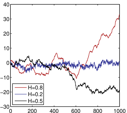
Figure 3: Examples of realizations of the fractional Brownian motion (fBm)for different values of the self-similar index $H$. For $\lx@glossaries@gls@link{main}{hurst}{\leavevmode H}=0.8$, the increments of the trajectory are positively correlated which results in a persistent motion. The oBm with uncorrelated increments is retrieved for $\lx@glossaries@gls@link{main}{hurst}{\leavevmode H}=0.5$ and for $\lx@glossaries@gls@link{main}{hurst}{\leavevmode H}=0.2$, the increments of the trajectory are anti-correlated which results in a anti-persistent motion.

In the framework of the generalized Langevin equation (GLE), it is possible to find the fBm as a solution by using a random force with long-range correlations, namely with a power-law correlation function. The memory kernel, $\beta(t)$, is then found with the fluctuation-dissipation theorem (eq. (40)) and, consequently, also have a power-law form. When the random force is chosen to be the fractional Gaussian noise (fGn), the GLE can be written as a fractional differential equation[Jeon2010], however, the solution of this equation is limited to the subdiffusive and diffusive case. From the physical point of view, the superdiffusive case is found only when the random force is “external”, meaning that the fluctuation-dissipation theorem does not hold and that the driving noise and the dissipation may have different origins, which may be the case in nonequilibrium systems[Porr1996].

It is possible to find the propagator of the fBm by using the method of path integrals[Calvo2008], borrowed from quantum mechanics (note that Shrödinger’s equation resembles a diffusion equation with an imaginary diffusion coefficient). The propagator, given by

$$G_{H}(x,t)=\sqrt{\frac{H}{\pi}}\frac{\operatorname{\Gamma}(H+1/2)}{t^{H}}\exp\left[-H\operatorname{\Gamma}^{2}(H+1/2)\frac{x^{2}}{t^{2H}}\right],$$ (52)

is a Gaussian function with a variance proportional to $t^{2H}$. It has the same form than the propagator of the oBm (eq. (13)) but with a “stretched” time $t^{2H}$. The transport equation of the fBm is easily found from the Fourier transform of eq. (52) to be

$$\frac{\text{\rotatebox[origin={t}]{13.0}{\scalebox{0.95}[1.0]{$\partial$}}}}{\text{\rotatebox[origin={t}]{13.0}{\scalebox{0.95}[1.0]{$\partial$}}}t}n(x,t)=D_{\beta}t^{\beta-1}\frac{\text{\rotatebox[origin={t}]{13.0}{\scalebox{0.95}[1.0]{$\partial$}}}^{2}}{\text{\rotatebox[origin={t}]{13.0}{\scalebox{0.95}[1.0]{$\partial$}}}x^{2}}n(x,t),$$ (53)

where $0<\beta=2\lx@glossaries@gls@link{main}{hurst}{\leavevmode H}<2$ and $D_{\beta}=(2\operatorname{\Gamma}^{2}(H+1/2))^{-1}$ is a stretched diffusion coefficient of dimensions $[m^{2}/s^{\beta}]$. This equation is called the stretched time diffusion equation[Mainardi2010]. By using the rule

$$\frac{\text{\rotatebox[origin={t}]{13.0}{\scalebox{0.95}[1.0]{$\partial$}}}}{\text{\rotatebox[origin={t}]{13.0}{\scalebox{0.95}[1.0]{$\partial$}}}t^{\beta}}=\beta t^{\beta-1}\frac{\text{\rotatebox[origin={t}]{13.0}{\scalebox{0.95}[1.0]{$\partial$}}}}{\text{\rotatebox[origin={t}]{13.0}{\scalebox{0.95}[1.0]{$\partial$}}}t},$$ (54)

it can be interpreted as the result of the classical diffusion equation with a stretched time.

We note that the Langevin approach and the CTRW approach are not equivalent in the non-Markovian case. Equation (53) is local in time, whereas eq. (27) with $\alpha=2,\beta<1$, the time-fractional diffusion equation, is not. In the fBm case, the non-Markovian character is provided by a time dependent diffusivity $D=D_{0}t^{\beta-1}$. Moreover, The solution of eq. (53) is Gaussian, while the solution of the time-fractional diffusion equation is not; it is given by the transcendental functions known as the M-Wright function which tends to the Gaussian function for $\beta=1$[Mainardi2010].

2.2.2 Fractional Lévy motion

Here, we discuss the fractional Lévy motion (fLm), which is a generalization of the fBm, including both long-range temporal dependence and non-Gaussian statistics.

The stochastic equation defining the fLm process is[Laskin2002, Calvo2009]

$$x_{\lx@glossaries@gls@link{main}{alpha}{\leavevmode\alpha},H}(t)=\frac{1}{\operatorname{\Gamma}\left(H-1/\lx@glossaries@gls@link{main}{alpha}{\leavevmode\alpha}+1\right)}\int_{0}^{t}(t-t^{\prime})^{H-1/\lx@glossaries@gls@link{main}{alpha}{\leavevmode\alpha}}\xi_{\lx@glossaries@gls@link{main}{alpha}{\leavevmode\alpha},\sigma}(t^{\prime})\operatorname{d}t^{\prime}\mbox{,}$$ (55)

where $\xi_{\lx@glossaries@gls@link{main}{alpha}{\leavevmode\alpha},\sigma}(t)$ is an uncorrelated noise distributed according to a Lévy symmetric, strictly stable distribution, with index of stability α, ($0<\lx@glossaries@gls@link{main}{alpha}{\leavevmode\alpha}\leq 2$) and scale parameter $\sigma$. From the properties of α-stable random variable, we have $x_{\lx@glossaries@gls@link{main}{alpha}{\leavevmode\alpha},H}(\lambda t)=\lambda^{H}x_{\lx@glossaries@gls@link{main}{alpha}{\leavevmode\alpha},H}(t)$, with $\lx@glossaries@gls@link{main}{hurst}{\leavevmode H}=\lx@glossaries@gls@link{main}{beta}{\leavevmode\beta}/\lx@glossaries@gls@link{main}{alpha}{\leavevmode\alpha}$. Therefore, the fLm belongs to the important family of $H$-self similar process with stationary increments (also abbreviated H-sssi), like the fBm. Consequently, the moments of $x_{\lx@glossaries@gls@link{main}{alpha}{\leavevmode\alpha},H}(t)$ exhibit the desired general non-classical feature

$$\left\langle|x_{\lx@glossaries@gls@link{main}{alpha}{\leavevmode\alpha},H}(t)|^{s}\right\rangle\propto t^{sH},$$ (56)

where $0<s<\lx@glossaries@gls@link{main}{alpha}{\leavevmode\alpha}$, to ensure convergence of the moments. For a non-degenerated process, the values of $H$ are restricted to[Samorodnitsky1994]

$$\left\{\begin{array}[]{lll}0<H\leq 1/\lx@glossaries@gls@link{main}{alpha}{\leavevmode\alpha}&\mbox{ if }&\lx@glossaries@gls@link{main}{alpha}{\leavevmode\alpha}<1\mbox{,}\\ 0<H\leq 1&\mbox{ if }&\lx@glossaries@gls@link{main}{alpha}{\leavevmode\alpha}\geq 1\mbox{.}\end{array}\right.$$ (57)

The long-term memory is engendered by the convolution with the power-law kernel and the non-Gaussian statistics by the Lévy noise. The fLm generalizes the fractional Brownian motion (fBm)[Mandelbrot1968]. Indeed, for $\lx@glossaries@gls@link{main}{alpha}{\leavevmode\alpha}=2$, the noise has a Gaussian distribution and the process is the fBm. When $\lx@glossaries@gls@link{main}{hurst}{\leavevmode H}=1/\lx@glossaries@gls@link{main}{alpha}{\leavevmode\alpha}$ the process is time-uncorrelated and when $\lx@glossaries@gls@link{main}{hurst}{\leavevmode H}<1/\lx@glossaries@gls@link{main}{alpha}{\leavevmode\alpha}$ or $\lx@glossaries@gls@link{main}{hurst}{\leavevmode H}>1/\lx@glossaries@gls@link{main}{alpha}{\leavevmode\alpha}$ the process exhibits negative or positive time correlations, respectively. Therefore, for $\lx@glossaries@gls@link{main}{alpha}{\leavevmode\alpha}=2$ and $\lx@glossaries@gls@link{main}{hurst}{\leavevmode H}=1/2$, one recovers the oBm corresponding to classical diffusion (eq. (45)).

Figure 4: Examples of propagators for different parameters of the fLm for times $t_{i}=1,2,...,9$ and effective diffusivity $K=1$. a: Subdiffusive case with $\lx@glossaries@gls@link{main}{alpha}{\leavevmode\alpha}=2$ (Gaussian) and $\lx@glossaries@gls@link{main}{beta}{\leavevmode\beta}=0.5$ (anti-correlated) ($\lx@glossaries@gls@link{main}{hurst}{\leavevmode H}=0.25$). b: Diffusive case with $\lx@glossaries@gls@link{main}{alpha}{\leavevmode\alpha}=2$ (Gaussian) and $\lx@glossaries@gls@link{main}{beta}{\leavevmode\beta}=1$ (uncorrelated) ($\lx@glossaries@gls@link{main}{hurst}{\leavevmode H}=0.5$). c: Superdiffusive case with $\lx@glossaries@gls@link{main}{alpha}{\leavevmode\alpha}=1$ (Lévy stable) and $\lx@glossaries@gls@link{main}{beta}{\leavevmode\beta}=1$ (uncorrelated) ($\lx@glossaries@gls@link{main}{hurst}{\leavevmode H}=1$).

Using path integrals, Calvo, Sánchez and Carreras have shown that the transport equation of the fLm process is a space-fractional diffusion equation with time dependent diffusivity[Calvo2009]

$$\frac{\text{\rotatebox[origin={t}]{13.0}{\scalebox{0.95}[1.0]{$\partial$}}}}{\text{\rotatebox[origin={t}]{13.0}{\scalebox{0.95}[1.0]{$\partial$}}}t}n(x,t)=Kt^{\lx@glossaries@gls@link{main}{beta}{\leavevmode\beta}-1}\frac{\text{\rotatebox[origin={t}]{13.0}{\scalebox{0.95}[1.0]{$\partial$}}}^{\alpha}}{\text{\rotatebox[origin={t}]{13.0}{\scalebox{0.95}[1.0]{$\partial$}}}\left|x\right|^{\alpha}}n(x,t)\mbox{.}$$ (58)

Here $n(x,t)$ is the density of particles, $K$ is an effective diffusion coefficient and α and β are the space and time transport exponents, respectively, with $\lx@glossaries@gls@link{main}{hurst}{\leavevmode H}=\lx@glossaries@gls@link{main}{beta}{\leavevmode\beta}/\lx@glossaries@gls@link{main}{alpha}{\leavevmode\alpha}$. The space derivative of order α is the Riesz fractional differential operator[Podlubny1999] (appendix LABEL:sec:fract_ope). The restriction on the range of permissible values for $H$ (eq. (57)) translates for β as

$$\left\{\begin{array}[]{lll}0<\lx@glossaries@gls@link{main}{beta}{\leavevmode\beta}\leq 1&\mbox{ if }&\lx@glossaries@gls@link{main}{alpha}{\leavevmode\alpha}<1\mbox{,}\\ 0<\lx@glossaries@gls@link{main}{beta}{\leavevmode\beta}\leq\lx@glossaries@gls@link{main}{alpha}{\leavevmode\alpha}&\mbox{ if }&\lx@glossaries@gls@link{main}{alpha}{\leavevmode\alpha}\geq 1\mbox{.}\end{array}\right.$$ (59)

When $\lx@glossaries@gls@link{main}{beta}{\leavevmode\beta}<1$ or $\lx@glossaries@gls@link{main}{beta}{\leavevmode\beta}>1$ the process is negatively or positively time correlated, $\lx@glossaries@gls@link{main}{beta}{\leavevmode\beta}=1$ corresponding to an uncorrelated process.

The propagator of eq. (58) is a Lévy distribution which depends on $x/t^{H}$[Calvo2009]

$$G_{\lx@glossaries@gls@link{main}{alpha}{\leavevmode\alpha},\lx@glossaries@gls@link{main}{beta}{\leavevmode\beta}}(x,t)=\frac{C(\lx@glossaries@gls@link{main}{alpha}{\leavevmode\alpha},\lx@glossaries@gls@link{main}{beta}{\leavevmode\beta})}{t^{\lx@glossaries@gls@link{main}{beta}{\leavevmode\beta}/\lx@glossaries@gls@link{main}{alpha}{\leavevmode\alpha}}}L_{\lx@glossaries@gls@link{main}{alpha}{\leavevmode\alpha},\sigma}\left[C(\lx@glossaries@gls@link{main}{alpha}{\leavevmode\alpha},\lx@glossaries@gls@link{main}{beta}{\leavevmode\beta})\frac{x}{t^{\lx@glossaries@gls@link{main}{beta}{\leavevmode\beta}/\lx@glossaries@gls@link{main}{alpha}{\leavevmode\alpha}}}\right],$$ (60)

where $C(\lx@glossaries@gls@link{main}{alpha}{\leavevmode\alpha},\lx@glossaries@gls@link{main}{beta}{\leavevmode\beta})=\lx@glossaries@gls@link{main}{beta}{\leavevmode\beta}^{1/\lx@glossaries@gls@link{main}{alpha}{\leavevmode\alpha}}\operatorname{\Gamma}\left(\frac{\lx@glossaries@gls@link{main}{beta}{\leavevmode\beta}-1}{\lx@glossaries@gls@link{main}{alpha}{\leavevmode\alpha}}+1\right)$ and $\sigma =K{}^{1/\text{<span title="" class="ltx\_glossaryref ltx\_font\_italic" style="font-size:70\%;">α</span>}}\mathrm{\Gamma }(\frac{\text{<span title="" class="ltx\_glossaryref"><span class="ltx\_text ltx\_glossary\_name"><xmath xmlns="http://dlmf.nist.gov/LaTeXML" id="S2.SS2.SSS2.p4.3.m2.1.7.2.1d" xref="S2.SS2.SSS2.p4.3.m2.1.7.2.1f.cmml"><xmtok name="beta" role="UNKNOWN" font="italic" id="S2.SS2.SSS2.p4.3.m2.1.7.2.1e" xref="S2.SS2.SSS2.p4.3.m2.1.7.2.1f.cmml">β</xmtok></xmath></span></span>}}{}$