Approximate solution of a system of singular integral equations of the first kind by using Chebyshev polynomials

Abstract

The aim of the present work is to introduce a method based on Chebyshev polynomials for the numerical solution of a system of Cauchy type singular integral equations of the first kind on a finite segment. Moreover, an estimation error is computed for the approximate solution. Numerical results demonstrate effectiveness of the proposed method.

1 Introduction

Let us consider a system of singular integral equations of the form

$$A(t)\Phi(t)+\int_{-1}^{1}\frac{B(\tau)\Phi(\tau)}{\tau-t}\,d\tau+\int_{-1}^{1}K(t,\tau)\Phi(\tau)d\tau=F(t)\,, -1<t<1$$ (1)

where

$$K(t,\tau)=\left[K_{ij}(t,\tau)\right],\,\,\,\,i,j=1,2,\ldots,N\,,$$

$$F(t)=[f_{1}(t)\,,\,f_{2}(t)\,,\,\ldots\,,\,f_{N}(t)]^{T}\,,$$

$$\Phi(t)=[\phi_{1}(t)\,,\,\phi_{2}(t)\,,\,\ldots\,,\,\phi_{N}(t)]^{T}\,,$$

$$A(t)=\left[a_{ij}(t)\right]\,,\,\,\,\,i,j=1,2,\ldots,N\,,$$

$$B(t)=\left[b_{ij}(t)\right]\,,\,\,\,\,i,j=1,2,\ldots,N\,.$$

Here, $\{K_{ij}(t,\tau)\}_{i,j=1}^{N}$ and $\{f_{i}(t)\}_{i=1}^{N}$ are given real-valued H$\ddot{o}$lder functions and $\{\phi_{j}(t)\}_{j=1}^{N}$ are the unknown functions. The matrices $A$ and $B$ are known such that $S=A+B$ and $D=A-B$ are nonsingular for all $t\in[-1,1]$. In some familiar physical problems the entries of the matrices $A$ and $B$ are constants.

The singular integral equations play important roles in physics and theoretical mechanics, particularly in the areas of elasticity, aerodynamics, and unsteady aerofoil theory. They are highly effective in solving boundary value problems occurring in the theory of functions of a complex variable, potential theory, the theory of elasticity, and the theory of fluid mechanics. A general theory of the system of equations (1) has given in mu .

We study the system (1) in the case that $A(t)=0$ and $B(t)$ is a constant matrix. Therefore, the $i^{th}$ equation of system (1) takes the form

$$\int_{-1}^{1}\sum_{j=1}^{N}b_{ij}\phi_{j}(\tau)\frac{d\tau}{\tau-t}\,+\int_{-1}^{1}\sum_{j=1}^{N}K_{ij}(t,\tau)\phi_{j}(\tau)d\tau=f_{i}(t)\,,\ \ \ -1<t<1\,.$$ (2)

Studies on this singular integral equation can be found in some literatures (See ab ; cb ; kp ; ks ). Chakrabarti and Berghe cb proposed a method for solving Eq. (2) using polynomial approximation and collocation points have chosen to be the zeros of the Chebyshev polynomials of the first kind for all cases. Kashfi and Shahmorad ks constructed another approximate solution of this equation using Chebyshev polynomials of the first and second kinds. Some other methods for solving this equation can be found in ab ; kp . A convergence analysis of Galerkin and collocation methods for Eq. (2) has been given by Miel mi .

A special type of Eq. (2) is the famous Cauchy singular integral equation

$$\int_{-1}^{1}\frac{\phi(\tau)}{\tau-t}\,d\tau=f(t)\,,\ \ \ -1<t<1\,,$$ (3)

which has the following analytical solutions in four special cases based on boundedness of the unknown function $\phi(\tau)$ at the endpoints of the interval $[-1,\,1]$ cb ; mc ; se .

Case 1. If the function $\phi(\tau)$ is unbounded at the endpoints $\tau=\pm 1$, then

$$\phi(\tau)=\frac{a_{0}}{\sqrt{1-\tau^{2}}}-\frac{1}{{\pi}^{2}\sqrt{1-\tau^{2}}}\int_{-1}^{1}\frac{\sqrt{1-t^{2}}f(t)}{t-\tau}\,dt\,,\ \ \ -1<\tau<1$$ (4)

where $a_{0}$ is an arbitrary constant.

Case 2. If the function $\phi(\tau)$ is bounded at the endpoints $\tau=\pm 1$, then

$$\phi(\tau)=-\frac{\sqrt{1-\tau^{2}}}{{\pi}^{2}}\int_{-1}^{1}\frac{f(t)}{\sqrt{1-t^{2}}\,(t-\tau)}\,dt\,,\ \ \ -1<\tau<1$$ (5)

a necessary and sufficient condition of existing this solution is:

$$\int_{-1}^{1}\frac{f(t)}{\sqrt{1-t^{2}}}\,dt=0\,.$$ (6)

Case 3. If the function $\phi(\tau)$ is bounded at the endpoint $\tau=-1$ and unbounded at the endpoint $\tau=1$, then

$$\phi(\tau)=-\frac{1}{{\pi}^{2}}\,\sqrt{\frac{1+\tau}{1-\tau}}\,\int_{-1}^{1}\sqrt{\frac{1-t}{1+t}}\frac{f(t)}{t-\tau}\,dt\,, -1<\tau<1.$$ (7)

Case 4. If the function $\phi(\tau)$ is bounded at the endpoint $\tau=1$ and unbounded at the endpoint $\tau=-1$, then

$$\phi(\tau)=-\frac{1}{{\pi}^{2}}\,\sqrt{\frac{1-\tau}{1+\tau}}\,\int_{-1}^{1}\sqrt{\frac{1+t}{1-t}}\frac{f(t)}{t-\tau}\,dt\,, -1<\tau<1.$$ (8)

More methods for solving Eq. (3) have given in en ; lz ; se ; ts .

In the next section, we investigate approximate solutions for system (1) in the above four cases.

2 Approximate solution

To find approximate solutions for system (1) in cases 1,2,3,4, for $\nu\in\{1,2,3,4\}$ we set

$$\phi_{j}(\tau)\simeq\varphi_{\nu,j}(\tau):=\frac{\lambda_{\nu}(\tau)}{\sqrt{1-{\tau}^{2}}}\sum_{l=0}^{M}\beta_{jl}\,P_{\nu,l}(\tau)\,,\ \ \ j=1,2,\ldots,N$$ (9)

and

$$K_{ij}(t,\tau):=\sum_{k=0}^{M}\gamma_{ijk}(t)\,P_{\nu,k}(\tau)\,,\ \ \ \ i,j=1,2,\ldots,N\,,$$ (10)

where

$$P_{\nu,j}(x)=\left\{\begin{array}[]{cc}T_{j}(x)=\cos(j\theta),&\nu=1,\\ \\ U_{j}(x)=\frac{\sin\left((j+1)\theta\right)}{\sin(\theta)},&\nu=2,\\ \\ V_{j}(x)=\frac{\cos\left((j+\frac{1}{2})\theta\right)}{\cos(\frac{\theta}{2})},&\nu=3,\\ \\ W_{j}(x)=\frac{\sin\left((j+\frac{1}{2})\theta\right)}{\sin(\frac{\theta}{2})},&\nu=4,\end{array}\right.$$

are the Chebyshev polynomials of the first to fourth kinds and

$$\lambda_{\nu}(t)=\left\{\begin{array}[]{cc}1,&\nu=1,\\ 1-t^{2},&\nu=2,\\ 1+t,&\nu=3,\\ 1-t,&\nu=4,\end{array}\right.$$

in which $x=\cos(\theta)$. The roots of Chebyshev polynomials $P_{\nu,M+1}(x)$ are given by

$$x_{\nu,n}=\left\{\begin{array}[]{cc}\cos\left(\frac{(2n-1)\pi}{2(M+1)}\right),&\nu=1,\\ \\ \cos\left(\frac{n\pi}{M+2}\right),&\nu=2,\\ \\ \cos\left(\frac{(2n-1)\pi}{2M+3}\right),&\nu=3,\\ \\ \cos\left(\frac{2n\pi}{2M+3}\right),&\nu=4,\end{array}\right.$$ (20)

where $n=1,2,\ldots\,,M+1$. These roots are used as the nods of Gauss-Chebyshev quadrature rules.
Lemma.mh The Chebyshev polynomials satisfy the orthogonality property

$$\int_{-1}^{1}\frac{\lambda_{\nu}(t)}{\sqrt{1-t^{2}}}P_{\nu,i}(t)P_{\nu,j}(t)\,dt\,=\left\{\begin{array}[]{lll}0,&i\neq j,\\ \\ \pi,&i=j=0\,,&\nu=1,\\ \\ \frac{\pi}{2},&i=j\neq 0,&\nu=1,\\ \\ \frac{\pi}{2},&i=j,&\nu=2,\\ \\ {\pi},&i=j,&\nu=3\,,\,4.\end{array}\right.$$ (21)

Theorem 1.mh As a Cauchy principle value integral, we have

$$\int_{-1}^{1}\frac{\lambda_{\nu}(\tau)}{\sqrt{1-\tau^{2}}}\,\frac{P_{\nu,j}(\tau)}{\tau-t}\,d\tau\,={\pi}\,\left\{\begin{array}[]{cc}U_{j-1}(t),&\nu=1,\\ \\ -T_{j+1}(t),&\nu=2,\\ \\ W_{j}(t),&\nu=3,\\ \\ -V_{j}(t),&\nu=4.\end{array}\right.$$ (29)

Now we describe details of finding approximate solution in cases 1-4.

Case 1. For $\nu=1$ the relations (9)-(10) take the forms

$$\phi_{j}(\tau)\simeq\varphi_{1,j}(\tau):=\frac{1}{\sqrt{1-{\tau}^{2}}}\sum_{l=0}^{M}{}^{{}^{\prime}}\beta_{jl}\,T_{l}(\tau)\,,\ \ \ \ j=1,2,\ldots,N$$ (30)

and

$$K_{ij}(t,\tau):=\sum_{k=0}^{M}{}^{{}^{\prime}}\gamma_{ijk}(t)\,T_{k}(\tau)\,,\ \ \ \ \ i,j=1,2,\ldots,N$$ (31)

where $\beta_{jl}\ \ (j=1,2,\ldots,N,\ \ \ l=0,1,\ldots,M)$ are unknown coefficients and the symbol ($\sum{}^{{}^{\prime}}$) denotes that the first term in the summation is halved. The functions

$$\gamma_{ijk}(t)=\frac{2}{\pi}\int_{-1}^{1}\frac{K_{ij}(t,\tau)T_{k}(\tau)}{\sqrt{1-{\tau}2}}\,d\tau\,,\ \ \ \ i,j=1,2,\ldots,N,\ \ \ \ k=0,1,\ldots,M$$

can be determined exactly, or may be approximated by using Gauss-Chebyshev quadrature rule, i.e

$$\gamma_{ijk}(t)\simeq\frac{2}{M+1}\sum_{s=1}^{M+1}K_{ij}(t,x_{1,s})T_{k}(x_{1,s})\,,$$

where $x_{1,s}$ obtain from (20).

Substituting from (30)-(31) into Eq. (2) and using (21)-(29) for $\nu=1$, gives the system

$$\sum_{j=1}^{N}\sum_{l=1}^{M}b_{ij}\beta_{jl}U_{l-1}(t)+\frac{1}{2}\sum_{j=1}^{N}\sum_{k=0}^{M}{}^{{}^{\prime}}\gamma_{ijk}(t)\beta_{jk}=\frac{1}{\pi}f_{i}(t)\,,\ \ \ \ \ i=1,2,\ldots,N.$$ (32)

If the given functions $f_{i}(t)$ and $\gamma_{ijk}(t)$ are square integrable on $[-1\,,\,\,1]$ with respect to the weight function $\frac{\lambda_{1}(t)}{\sqrt{1-t^{2}}}$, then they can be expanded as

$$\left\{\begin{array}[]{lll}\gamma_{ijk}(t)\simeq\sum_{l=0}^{M-1}G_{ijkl}\,U_{l}(t)\,,&i,j=1,2,\ldots,N,&\ \ \ \ \ k=0\,,1\,,\ldots\,,M\\ \\ \frac{1}{\pi}f_{i}(t)\simeq\sum_{l=0}^{M-1}c_{il}\,U_{l}(t)\,,&i=1,2,\ldots,N,&\end{array}\right.$$ (33)

where the coefficients

$$\left\{\begin{array}[]{lll}G_{ijkl}&=\frac{2}{\pi}\int_{-1}^{1}\sqrt{1-t^{2}}\gamma_{ijk}(t)U_{l}(t)\,dt\\ &=\frac{4}{{\pi}^{2}}\int_{-1}^{1}\int_{-1}^{1}\sqrt{\frac{1-t^{2}}{1-{\tau}^{2}}}K_{ij}(t,\tau)U_{l}(t)\,T_{k}(\tau)\,d\tau dt&\\ &\ \ \ \ \ \ \ \ \ \ \ \ i,j=1,2,\ldots,N,\ \ \ k=0,1,\ldots,M\,,&l=0,1,\ldots,M-1\\ \\ \ c_{il}&=\frac{1}{{\pi}^{2}}\int_{-1}^{1}\sqrt{1-t^{2}}f_{i}(t)U_{l}(t)\,dt\,,\ \ i=1,2,\ldots,N,&l=0,1,\ldots,M-1,\end{array}\right.$$

can be approximately determined from

$$\left\{\begin{array}[]{ll}G_{ijkl}\simeq\frac{4}{(M+1)^{2}}\sum_{r=1}^{M}\sum_{s=1}^{M+1}(1-x_{2,r}^{2})K_{ij}(x_{2,r},x_{1,s})U_{l}(x_{2,r})T_{k}(x_{1,s})\,,\\ \\ c_{il}\simeq\frac{2}{\pi(M+1)}\sum_{r=1}^{M}(1-x_{2,r}^{2})f_{i}(x_{2,r})U_{l}(x_{2,r}).\end{array}\right.$$ (35)

Using (33) in (32) and linearly independence of $\{U_{l}(t)\}$, yield

$$\sum_{l=0}^{M-1}\sum_{j=1}^{N}b_{ij}\beta_{j\{l+1\}}U_{l}(t)+\frac{1}{2}\sum_{l=0}^{M-1}\sum_{j=1}^{N}\sum_{k=0}^{M}{}^{{}^{\prime}}G_{ijkl}\beta_{jk}U_{l}(t)=\sum_{l=0}^{M-1}c_{il}\,U_{l}(t),$$

which leads to the linear system

$$\sum_{j=1}^{N}\left[b_{ij}\beta_{j\{l+1\}}+\frac{1}{2}\sum_{k=0}^{M}{}^{{}^{\prime}}G_{ijkl}\beta_{jk}\right]=c_{il},\ \ i=1,2,\ldots,N,\ \ l=0,1,\ldots,M-1$$ (36)

for the unknown values $\beta_{jk}\ \ (j=1,2,\ldots,N,\ \ \ k=0,1,\ldots,M)$. By taking arbitrary values for example for $\beta_{11},\ldots,\beta_{N1}$, the remaining coefficients $\beta_{jk}$ are uniquely found via the linear system (36) which determine the elements of the vector function $\Phi(t)$ via Eq. (30).

Case 2. We set $\nu=2$ in (9)-(10) and substitute them in Eq. (2) to get

$$-\sum_{j=1}^{N}\sum_{l=0}^{M}b_{ij}\beta_{jl}T_{l+1}(t)+\frac{1}{2}\sum_{j=1}^{N}\sum_{k=0}^{M}\gamma_{ijk}(t)\beta_{jk}=\frac{1}{\pi}f_{i}(t)\,,\ \ \ \ \ i=1,2,\ldots,N.$$ (37)

where we used the formulae (21)-(29). Then, we expand the functions $f_{i}(t)$ and $\gamma_{ijk}(t)$ as

$$\left\{\begin{array}[]{lll}\gamma_{ijk}(t)\simeq\sum_{l=0}^{M}{}^{{}^{\prime}}G_{ijkl}\,T_{l}(t)\,,&i,j=1,2,\ldots,N,&k=0\,,1\,,\ldots\,,M\\ \\ \frac{1}{\pi}f_{i}(t)\simeq\sum_{l=0}^{M}{}^{{}^{\prime}}c_{il}\,T_{l}(t)\,,&\ i=1,2,\ldots,N&\end{array}\right.$$

where the coefficients are determined by

$$\left\{\begin{array}[]{ll}G_{ijkl}=\frac{2}{\pi}\int_{-1}^{1}\frac{1}{\sqrt{1-t^{2}}}\gamma_{ijk}(t)T_{l}(t)\,dt\,,\ \ \ \ \ i,j=1,2,\ldots,N,&k,l=0\,,1\,,\ldots\,,M\,,\\ \ \ \ \ \ \ \ =\frac{4}{{\pi}^{2}}\int_{-1}^{1}\int_{-1}^{1}\sqrt{\frac{1-\tau^{2}}{1-t^{2}}}K_{ij}(t,\tau)T_{l}(t)\,U_{k}(\tau)\,d\tau dt&\\ \\ c_{il}=\frac{2}{{\pi}^{2}}\int_{-1}^{1}\frac{1}{\sqrt{1-t^{2}}}f_{i}(t)T_{l}(t)\,dt\,,\ \ \ \ \ \ \ \ \ \ i=1,2,\ldots,N,&l=0\,,1\,,\ldots\,,M\end{array}\right.$$

or approximated by

$$\left\{\begin{array}[]{ll}G_{ijkl}\simeq\frac{4}{(M+1)(M+2)}\sum_{r=1}^{M+1}\sum_{s=1}^{M+1}(1-x_{2,s}^{2})K_{ij}(x_{1,r},x_{2,s})T_{l}(x_{1,r})U_{k}(x_{2,s})\,,\\ \\ c_{il}\simeq\frac{2}{\pi(M+1)}\sum_{r=1}^{M+1}f_{i}(x_{1,r})T_{l}(x_{1,r}).\end{array}\right.$$ (40)

Using the last expansions in Eq. (37), returns the following linear system of equations

$$\left\{\begin{array}[]{lll}\frac{1}{2}\sum_{j=1}^{N}\sum_{k=0}^{M}G_{ijkl}\beta_{jk}=c_{il},&i=1,2,\ldots\,,N,&l=0\\ \\ \sum_{j=1}^{N}\left\{-b_{ij}\beta_{j\{l-1\}}+\frac{1}{2}\sum_{k=0}^{M}G_{ijkl}\beta_{jk}\right\}=c_{il},&i=1,2,\ldots\,,N,&l=1,2,\ldots,M\end{array}\right.$$ (44)

for the unknown values $\beta_{jl}\ \ (j=1,2,\ldots,N,\ \ \ l=0,1,\ldots,M)$. Then the elements of the vector function $\Phi(t)$ obtain from Eq. (9).
Case 3,4. Proceeding by the same way as we did in cases $1,2$, we get the linear systems

$$\sum_{j=1}^{N}\left\{b_{ij}\beta_{jl}+\sum_{k=0}^{M}G_{ijkl}\beta_{jk}\right\}=c_{il},\ \ \ i=1,2,\ldots\,,N,\ \ \ l=0,1,\ldots,M$$ (45)

and

$$\sum_{j=1}^{N}\left\{-b_{ij}\beta_{jl}+\sum_{k=0}^{M}G_{ijkl}\beta_{jk}\right\}=c_{il},\ \ \ i=1,2,\ldots\,,N,\ \ \ l=0,1,\ldots,M$$ (46)

respectively for $\nu=3$ and $\nu=4$, and then we determine the elements of corresponding vector $\Phi(t)$ via (9).

3 An estimation error and numerical results

In this section, we describe an estimation error for the approximate solution. Let

$$\overline{\Phi}(t)=[\varphi_{1}(t)\,,\,\varphi_{2}(t)\,,\,\ldots\,,\,\varphi_{N}(t)]^{T}$$

be the vector of approximate solution of the system (1) and $E(t)=\overline{\Phi}(t)-\Phi(t)$ be the associated vector valued error function. Due to the approximation $\overline{\Phi}(t)$, for $A(t)=0$ the system (1) may be written as

$$\int_{-1}^{1}\frac{B(\tau)\overline{\Phi}(\tau)}{\tau-t}\,d\tau+\int_{-1}^{1}K(t,\tau)\overline{\Phi}(\tau)d\tau=F(t)+H(t)\,,\ \ \ \ -1<t<1,$$ (47)

where the perturbation term $H(t)$ obtains from

$$H(t)=\int_{-1}^{1}\frac{B(\tau)\overline{\Phi}(\tau)}{\tau-t}\,d\tau+\int_{-1}^{1}K(t,\tau)\overline{\Phi}(\tau)d\tau-F(t)\,,\ \ \ \ \ -1<t<1.$$ (48)

Subtracting Eq. (47) from Eq. (1), yields a system of error equations as

$$\int_{-1}^{1}\frac{B(\tau){E(\tau)}}{\tau-t}\,d\tau+\int_{-1}^{1}K(t,\tau){E(\tau)}d\tau=H(t)\,,\ \ \ \ -1<t<1$$ (49)

which is solvable approximately like the system (1).

The following examples illustrate application of the method.

Example $1.$ Let

$$A(t)=0,\ \ \ B(t)=\left(\begin{array}[]{cc}1&\ \ 0\\ 0&\ \ 1\\ \end{array}\right),\ \ \ K(t,\tau)=\left(\begin{array}[]{cc}\tau-t&\ \ t\\ \tau&\ \ \tau+t\\ \end{array}\right),\ \ \ \ f_{1}(t)=\pi,\ \ \ f_{2}(t)=2\pi t$$

and find the solution of system (1) in case 1.

By the above information the system (1) reduces to

$$\left\{\begin{array}[]{ll}\int_{-1}^{1}\frac{\phi_{1}(\tau)}{\tau-t}\,d\tau+\int_{-1}^{1}(\tau-t)\phi_{1}(\tau)d\tau+\int_{-1}^{1}t\phi_{2}(\tau)d\tau=\pi,&-1<t<1\\ \\ \int_{-1}^{1}\frac{\phi_{2}(\tau)}{\tau-t}\,d\tau+\int_{-1}^{1}\tau\phi_{1}(\tau)d\tau+\int_{-1}^{1}(\tau+t)\phi_{2}(\tau)d\tau=2\pi t,&-1<t<1\end{array}\right.$$ (51)

since the matrices $S=A+B=I_{2}$ and $D=A-B=-I_{2}$ are nonsingular, therefore the solution of system (51) exists. The kernels $K_{1j}(t,\tau)$, $K_{2j}(t,\tau)$ ($j=1,2$), and the functions $f_{1}(t)$, $f_{2}(t)$ are polynomials of degree at most $1$, so we set

$$\phi_{j}(\tau):=\frac{1}{\sqrt{1-{\tau}^{2}}}\left\{\beta_{j0}\,T_{0}(\tau)+\beta_{j1}\,T_{1}(\tau)+\beta_{j2}\,T_{2}(\tau)\right\}\,,\ \ \ \ j=1,2$$ (52)

and

$$\begin{array}[]{lll}K_{ij}(t,\tau)=\gamma_{ij0}(t)T_{0}(\tau)+\gamma_{ij1}(t)T_{1}(\tau)\,,&i,j=1,2\\ f_{i}(t)=c_{i0}U_{0}(t)+c_{i1}U_{1}(t),&i=1,2&\end{array}$$

where

$$\begin{array}[]{cccc}\gamma_{110}(t)=-\frac{1}{2}U_{1}(t),&\gamma_{111}(t)=U_{0}(t),&\gamma_{120}(t)=\frac{1}{2}U_{1}(t),&\gamma_{121}(t)=0,\\ \gamma_{210}(t)=0,&\gamma_{211}(t)=U_{0}(t),&\gamma_{220}(t)=\frac{1}{2}U_{1}(t),&\gamma_{221}(t)=U_{0}(t),\\ c_{10}(t)=1,&c_{11}(t)=0,&c_{20}(t)=0,&c_{21}(t)=1.\\ \end{array}$$

Substituting these expansions into (51) and using (21)-(29), for $\nu=1,$ we obtain

$$\left\{\begin{array}[]{ll}\beta_{11}U_{0}(t)+\beta_{12}U_{1}(t)-\frac{1}{2}\beta_{10}U_{1}(t)+\frac{1}{2}\beta_{11}U_{0}(t)+\frac{1}{2}\beta_{20}U_{1}(t)=U_{0}(t)\\ \\ \beta_{21}U_{0}(t)+\beta_{22}U_{1}(t)+\frac{1}{2}\beta_{11}U_{0}(t)+\frac{1}{2}\beta_{20}U_{1}(t)+\frac{1}{2}\beta_{21}U_{0}(t)=U_{1}(t)\\ \end{array}\right.$$ (55)

Then the linear independency of $\{U_{0}(t),\ U_{1}(t)\}$ implies

$$\left\{\begin{array}[]{c}\frac{3}{2}\beta_{11}=1\\ -\frac{1}{2}\beta_{10}+\beta_{12}+\frac{1}{2}\beta_{20}=0\\ \frac{1}{2}\beta_{11}+\frac{3}{2}\beta_{21}=0\\ \frac{1}{2}\beta_{20}+\beta_{22}=1.\\ \end{array}\right.$$

A nonunique solution of this system for the arbitrary values of $\beta_{10}$ and $\beta_{20}$ is given by

$$\beta_{10},\ \ \ \beta_{11}=\frac{2}{3},\ \ \ \beta_{12}=\frac{1}{2}\left(\beta_{10}-\beta_{20}\right),\ \ \ \beta_{20},\ \ \ \beta_{21}=-\frac{2}{9},\ \ \ \beta_{22}=1-\frac{1}{2}\beta_{20}.$$

For example, if $\beta_{10}=\beta_{20}=2$, then $\beta_{12}=\beta_{22}=0$ and so we find from (52)

$$\phi_{1}(\tau)=\frac{\frac{2}{3}\tau+2}{\sqrt{1-\tau^{2}}}\,,\ \ \ \ \ \ \phi_{2}(\tau)=\frac{-\frac{2}{9}\tau+2}{\sqrt{1-\tau^{2}}}\,,$$

(See figure 1 for the behavior of these solutions).

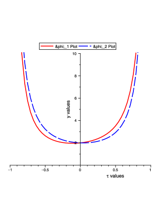
Figure 1: The plots of approximate solutions of Example 1 for M=2.

Example $2.$ Solve the problem of Example $1$ in case 3.

In this case, we set

$$\phi_{j}(\tau):=\sqrt{\frac{1+\tau}{1-\tau}}\left\{\beta_{j0}\,V_{0}(\tau)+\beta_{j1}\,V_{1}(\tau)\right\}\,,\ \ \ \ j=1,2$$ (57)

and

$$\begin{array}[]{lll}K_{ij}(t,\tau)=\gamma_{ij0}(t)V_{0}(\tau)+\gamma_{ij1}(t)V_{1}(\tau)\,,&i,j=1,2,\\ f_{i}(t)=c_{i0}W_{0}(t)+c_{i1}W_{1}(t),&i=1,2,&\end{array}$$

where

$$\begin{array}[]{cccc}\gamma_{110}(t)=W_{0}(t)-\frac{1}{2}W_{1}(t),&\gamma_{111}(t)=\gamma_{210}(t)=\gamma_{211}(t)=\gamma_{221}(t)=\frac{1}{2}W_{0}(t),\\ \gamma_{120}(t)=-\frac{1}{2}W_{0}(t)+\frac{1}{2}W_{1}(t),&\gamma_{121}(t)=0,\ \ \ \ \gamma_{220}(t)=\frac{1}{2}W_{1}(t),\\ c_{10}(t)=1,\ \ \ \ \ \ c_{11}(t)=0,&c_{20}(t)=-1,\ \ \ \ \ \ c_{21}(t)=1.\end{array}$$

Substituting these expansions into (51) and using (21)-(29) for $\nu=3$, result

$$\left\{\begin{array}[]{ll}\beta_{10}W_{0}(t)+\beta_{11}W_{1}(t)+\beta_{10}W_{0}(t)-\frac{1}{2}\beta_{10}W_{1}(t),\\ \ \ \ \ \ \ \ \ \ \ \ \ \ \ \ \ \ \ \ +\frac{1}{2}\beta_{11}W_{0}(t)-\frac{1}{2}\beta_{20}W_{0}(t)+\frac{1}{2}\beta_{20}W_{1}(t)=W_{0}(t)\\ \\ \beta_{20}W_{0}(t)+\beta_{21}W_{1}(t)+\frac{1}{2}\beta_{10}W_{0}(t)+\frac{1}{2}\beta_{11}W_{0}(t)\\ \ \ \ \ \ \ \ \ \ \ \ \ \ \ \ \ \ \ \ \ \ \ \ +\frac{1}{2}\beta_{20}W_{1}(t)+\frac{1}{2}\beta_{21}W_{0}(t)=-W_{0}(t)+W_{1}(t)\end{array}\right.$$ (60)

and from the linear independency of $\{W_{0}(t),\ W_{1}(t)\}$, we get the algebraic system

$$\left\{\begin{array}[]{c}2\beta_{10}+\frac{1}{2}\beta_{11}-\frac{1}{2}\beta_{20}=1\\ -\frac{1}{2}\beta_{10}+\beta_{11}+\frac{1}{2}\beta_{20}=0\\ \frac{1}{2}\beta_{10}+\frac{1}{2}\beta_{11}+\beta_{20}+\frac{1}{2}\beta_{21}=-1\\ \frac{1}{2}\beta_{20}+\beta_{21}=1,\\ \end{array}\right.$$

which has the unique solution

$$\beta_{10}=-\frac{10}{27}\,,\,\,\,\beta_{11}=\frac{28}{27}\,,\,\,\,\beta_{20}=-\frac{22}{9}\,,\,\,\,\beta_{21}=\frac{20}{9}\,,$$

and the solutions of (51) can be found via (57). The graphs of these solutions plotted in Fig. 2.

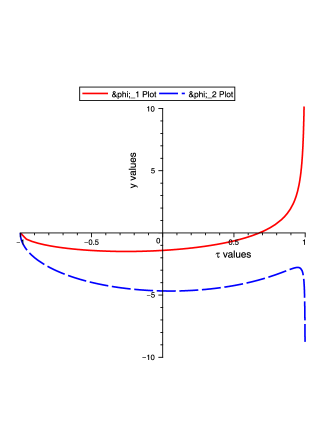
Figure 2: The plots of approximate solutions of Example 2 for M=2.

Example $3.$ Consider the problem of a half plane containing a crack parallel to the boundary which illustrated in Fig. 3 and formulated as the system eg

$$\left\{\begin{array}[]{ll}\int_{-1}^{1}\frac{\phi_{1}(\tau)}{\tau-t}\,d\tau+\int_{-1}^{1}\left[K_{11}(t,\tau)\phi_{1}(\tau)+K_{12}(t,\tau)\phi_{2}(\tau)d\tau\right]=0\\ \\ \int_{-1}^{1}\frac{\phi_{2}(\tau)}{\tau-t}\,d\tau+\int_{-1}^{1}\left[K_{21}(t,\tau)\phi_{1}(\tau)+K_{22}(t,\tau)\phi_{2}(\tau)d\tau\right]=\pi\end{array}\right.$$ (62)

with

$$K_{11}(t,\tau)=-\frac{\tau-t}{(\tau-t)^{2}+4h^{2}}+\frac{8h^{2}(\tau-t)}{\left[(\tau-t)^{2}+4h^{2}\right]^{2}}-\frac{4h^{2}(\tau-t)\left[12h^{2}-(\tau-t)^{2}\right]}{\left[(\tau-t)^{2}+4h^{2}\right]^{3}}\,,$$

$$K_{12}(t,\tau)=K_{21}(t,\tau)=-\frac{8h^{3}\left[4h^{2}-3(\tau-t)^{2}\right]}{\left[(\tau-t)^{2}+4h^{2}\right]^{3}}\,,$$

$$K_{22}(t,\tau)=-\frac{\tau-t}{(\tau-t)^{2}+4h^{2}}-\frac{8h^{2}(\tau-t)}{\left[(\tau-t)^{2}+4h^{2}\right]^{2}}-\frac{4h^{2}(\tau-t)\left[12h^{2}-(\tau-t)^{2}\right]}{\left[(\tau-t)^{2}+4h^{2}\right]^{3}},$$

where $h$ is the distance of crack from the boundary. The physical conditions of the problem impose that the relations

$$\int_{-1}^{1}\phi_{1}(\tau)\,d\tau=0\,,\ \ \ \ \int_{-1}^{1}\phi_{2}(\tau)\,d\tau=0$$ (63)

and

$$\phi_{1}(t)=\phi_{1}(-t),\ \ \ \phi_{2}(t)=-\phi_{2}(-t)$$

to be satisfied.

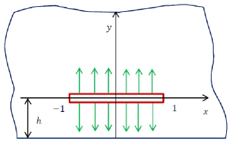
Figure 3: Crack parallel to a free boundary

Therefore the unknown functions may be expressed as

$$\phi_{1}(\tau)\simeq\frac{1}{\sqrt{1-\tau^{2}}}\,\sum_{j=0}^{M}\,\beta_{1j}\,T_{2j}(\tau),\ \ \ \ \phi_{2}(\tau)\simeq\frac{1}{\sqrt{1-\tau^{2}}}\,\sum_{j=1}^{M}\,\beta_{2j}\,T_{2j-1}(\tau).$$ (64)

For $\nu=1$, it follows from the orthogonality condition (21) that the second condition in (63) satisfies and the first one gives $\beta_{10}=0$.

By taking $\beta_{11}=\beta_{21}=0$, as arbitrary values, the remaining coefficients $\beta_{ij}$ are uniquely determined from the linear algebraic system (36) for each values of $h$ and $M.$ This leads us to find the functions $\phi_{1}(\tau)$ and $\phi_{2}(\tau)$ from (64).
The stress intensity factors

$$k_{1}=\lim_{\tau\rightarrow 1^{-}}\sqrt{1-\tau^{2}}\,\phi_{2}(\tau)$$

$$k_{2}=\lim_{\tau\rightarrow 1^{-}}\sqrt{1-\tau^{2}}\,\phi_{1}(\tau)$$

and their absolute estimation errors(Est.Err.) reported in table 1. For $h=\infty$ and $K_{ij}(t,\tau)=0,$ from Eqs. (64) and (35)-(36) the exact solutions of (62) are obtained as

$$\phi_{1}(\tau)=0,\ \ \ \ \ \phi_{2}(\tau)=\frac{\tau}{\sqrt{1-\tau^{2}}},$$

which give $k_{1}=1$ and $k_{2}=0$. This is shown in the last row of Table 1. The table shows the rapid convergence of the results even for relatively small values of $M$.

Table 1: Stress intensity factors for the crack parallel to the boundary

$h$	$M$	$k_{1}$	Est.Err. $k_{1}$	$k_{2}$	Est.Err. $k_{2}$
0.2	6	4.878800637605022	6.3e-14	1.750099102171126	6.2e-14
	7	4.788277537335018	1.1e-14	1.727809740547429	4.1e-15
	8	4.760729834685963	4.8e-14	1.719782910590219	1.1e-14
0.4	3	2.607272141646415	4.3e-15	0.7745787927510580	1.6e-16
	4	2.594500911475041	7.3e-15	0.7266641783709941	5.0e-15
	6	2.594423234973139	4.2e-14	0.7376171346942053	3.3e-16
0.6	2	1.834057544899021	1.1e-15	0.5664257041432605	4.1e-16
	5	1.960455689663461	6.1e-15	0.4297949760368867	1.6e-15
0.8	2	1.608371955353828	1.6e-15	0.3323260582700188	2.8e-16
	3	1.660617572058080	8.7e-16	0.2675691556476836	4.6e-16
1.0	2	1.461157081431933	2.0e-15	0.2104682299562445	1.1e-16
	4	1.485914720666516	2.1e-16	0.1796691052492212	1.1e-16
1.2	4	1.372176156193755	5.0e-16	0.1234414146531335	0.
1.5	4	1.262800608570183	1.6e-15	0.07465158121522054	1.7e-16
2.0	3	1.162112249974693	1.1e-15	0.03662808437088003	0.
3.0	2	1.077621553329114	3.3e-16	0.01274529646673066	0.
10	2	1.007451045420713	2.6e-16	0.00037197952964307	0.
$\infty$	1	1	0	0	0

4 Conclusions

We described a new idea of using Chebyshev polynomials for the numerical solution of system (1). As applications of this idea, we have solved the simple examples $1$ and $2$ as a coupled system of singular integral equations of the first kind. In example $3$, we studied a crack problem in solid mechanics and we reported the numerical results (see Table 1) to show the efficiency and rapid convergence of the proposed method for all these kinds of problems.

References

• (1) M. Abdolkawi, Solution of Cauchy type singular integral equations of the first kind by using differential transform method, Applied Mathematical Modelling, 39, pp. 2107-2118, (2015)
• (2) A. Chakrabarti, G. V. Berghe, Approximate solution of singular integral equations, Appl. Math. Lett., 17, pp. 533–559, (2004)
• (3) F. Erdogan, G. D. Gupta, T. S. Cook, in Mechanics of Fracture, Volume1, ed. by G. C. Sih, (Noordhoff International Publishing, Leyden, Netherlands, 1973), pp. 368-425, DOI:10.1007/978-94-017-2260-5
• (4) Z. K. Eshkuvatov, N. M. A. Nik Long, and M. Abdulkawi, Approximate solution of singular integral equations of the first kind with Cauchy kernel, Appl. Math. Lett., 22, pp. 651-657, (2009)
• (5) P. Karczmarek, D. Pylak, M. A. Sheshko, Application of Jacobi polynomials to approximate solution of a singular integral equation with Cauchy kernel, Appl. Math. Comput., 181, pp. 694 707, (2006)
• (6) M. Kashfi, S. Shahmorad, Approximate solution of a singular integral Cauchy-kernel equation of the first kind, Computational Methods in Applied Mathematics, 10(4), pp. 345-353, (2010)
• (7) D. Liu, X. Zhang, J. Wu, A collocation scheme for a certain Cauchy singular integral equation based on the superconvergence analysis, Appl. Math. Comput., 219, pp. 5198-5209, (2013)
• (8) B. N. Mandal, A. Chakrabarti, Applied Singular Integral Equations, Taylor and Francis Group, CRC Press, (2011)
• (9) J. C. Mason, D. C. Handscomb, Chebyshev Polynomials, (Chapman and Hall, CRC Press, 2003)
• (10) G. Miel, On the Galerkin and collocation methods for a Cauchy singular integral equation, SIAM J. NUMER. ANAL., 23(1), pp. 135-143, (1986)
• (11) N. I. Muskhelishvili, J. R. M. RADOK,Singular Integral Equations, (Wolters-Noordhoff Publishing Groningen, Netherlands, 1958), DOl:1 0.1007/978-94-009-9994-7
• (12) A. Setia, Numerical solution of various cases of Cauchy type singular integral equation, Appl. Math. Comput., 230, pp. 200-207, (2014)
• (13) J. L. Tsalamengas, A direct method to quadrature rules for a certain class of singular integrals with logarithmic, Cauchy, or Hadamard-type singularities, Int. J. Numer. Model., 25, pp. 512-524, (2012)