$G_{2}$ monopoles

Abstract

We investigate some aspects of Bogomolny-Prasad-Sommerfield monopole solutions in the Yang-Mills-Higgs theory with exceptional gauge group $G_{2}$ spontaneously broken to $U(1)\times U(1)$. Corresponding homotopy group is $\pi_{2}\left(G_{2}/U(1)\times U(1)\right)$ and similar to the $SU(3)$ theory, the $G_{2}$ monopoles are classified by two topological charges $(n_{1},n_{2})$. In fundamental representation these yield a subset of $SO(7)$ monopole configurations. Through inspection of the structure of $Alg(G_{2})$, we propose an extension of the Nahm construction to the $(n,1)_{G_{2}}$ monopoles. For $(1,1)_{G_{2}}$ monopole the Nahm data are written explicitly.

1 Introduction

Classical monopole solutions of spontaneously broken Yang-Mills-Higgs theories have long been the objects of detailed study. These topologically nontrivial field configurations may exist in gauge theories for an arbitrary semisimple compact Lie group [4, 5]. The simplest example is the ’t Hooft-Polyakov monopole in the $SU(2)$ theory [6, 7]. In the Bogomol’nyi-Prasad-Sommerfield (BPS) limit [8, 9] the potential of the scalar field is vanishing and the monopole solution is given by the first order equation which is integrable. Furthermore, the Bogomolny equation can be treated as dimensionally reduced self-duality equation and there is a duality between the monopole solutions of the Bogomolny equation and the matrix valued Nahm data [10]. The Nahm’s construction is a very powerful tool for constructing various multimonopoles in different models [11, 12, 13, 14, 15, 16], it also has a very interesting realization in the context of construction of D-branes [28].

Nahm’s construction can be generalized for all classical groups, as $SU(N)$ [14], symplectic and orthogonal groups [15, 16, 18]. Here we will concentrate on the case of the smallest simply connected compact exceptional group with a trivial center $G_{2}$. Topologically non-trivial boundary conditions of the scalar field yield nontrivial second homotopy group of the vacuum where the symmetry is broken to a residue group $H$, this there are monopole solutions of the $G_{2}$ Yang-Mills-Higgs theory.

Gauge theories with symmetry group $G_{2}$ have attracted much attention recently [19, 20, 21, 22, 23, 24, 31]. One of the reasons is that such a theory is similar to usual $SU(3)$ gluodynamics, thus it is useful to investigate how the center symmetry is relevant for deconfinement phase transition in the lattice $G_{2}$ gluodynamics [19, 20, 22, 23]. Recently, it was shown that in supersymmetric Yang-Mills theory, confinement-deconfinement transition does not break the symmetry of the $G_{2}$ ground state although the expectation value of the Wilson line exhibits a discontinuity [31].

On the other hand, the gauge group $G_{2}$ is the automorphism group of the division algebra of octonions. This property allows to construct octonionic instanton solution to the seven-dimensional $G_{2}$ Yang-Mills theory [24]. Also the massless monopole states in the $N=2$ supersymmetric Yang-Mills theory with symmetry group $G_{2}$ were considered recently [21].

Note that coupling of the gauge sector to the Higgs field in the seven-dimensional fundamental representation of $G_{2}$ may break this symmetry to $SU(3)$, however in this case some of fundamental monopoles, i.e. the monopoles associated with simple roots of the gauge group $G_{2}$, become massless (see e.g. [2]). In this paper we will mainly consider another, more simple situation, when the gauge symmetry is broken maximally by an adjoint Higgs mechanism to $U(1)\times U(1)$. In this case the monopoles have two topological charges with respect to either of the unbroken Abelian groups $U(1)$, thus the monopoles can be labeled by two integers $(n_{1},n_{2})$.

The organization of the paper is as follows. Section II is a review of the basic properties of the first exceptional group $G_{2}$, there we also review the Nahm’s formalism. Section III contains our results of construction of the $(1,1)_{G_{2}}$ monopoles. In Section IV we conclude with some additional remarks. In additional appendices we summarize the relevant information about the $\mathfrak{g}_{2}$ algebra and its representation.

2 Exceptional group $G_{2}$ and the Nahm construction

We start with some introductory remarks about the Lie group $G_{2}$. It is the smallest of the five exceptional simple Lie groups with trivial central element. Mathematically it can be thought as the group of automorphisms of the octonions or as a subgroup of the real orthogonal group $SO(7)$ which leaves one element of the 8-dimensional real spinor representation invariant. It is one of three simple Lie groups of rank two: $SU(3)$, $O(5)$ and $G_{2}$. The fundamental representation of $G_{2}$ is 7-dimensional, the number of generators of the corresponding algebra is 14 (we refer to the appendix A for details). Thus, the Cartan subgroup contains two commuting generators $H_{1},H_{2}$. The roots and coroots of the $G_{2}$ are shown in Fig. 1

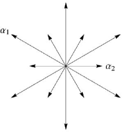
Figure 1: Root diagram of $G_{2}$ theory.

Explicitly, we can take the elements of the Cartan subalgebra $\mathbf{H}$

$$H_{1}=\leavevmode\nobreak\ \frac{1}{4}{\rm diag}(-1,1,-2,0,2,-1,1),\quad H_{2}=\leavevmode\nobreak\ \frac{1}{4\sqrt{3}}{\rm diag}(0,-1,1,0,-1,1,0);$$ (1)

so that the Killing form $\mathcal{K}(H_{i},H_{j})=\frac{1}{2}\delta_{ij}$.

Thereafter we consider the Yang-Mills-Higgs theory in the BPS limit. Then the monopoles are solutions of the first order Bogomol’nyi equation

$$D_{k}\Phi=B_{k}$$ (2)

The asymptotic value of the Higgs field along the positive direction of the third axis lies in the Cartan subalgebra: $\Phi_{\infty}=\mathbf{h}\cdot\mathbf{H}$. If the $G_{2}$ symmetry is maximally broken to $U(1)\times U(1)$, all roots have non vanishing inner product with vector $\mathbf{h}$ and, since $\pi_{1}(G_{2})=0$, the monopole solutions are classified according to the homotopy group $\pi_{2}(G_{2}/U(1)\times U(1))=\pi_{1}(U(1)\times U(1))=\mathbb{Z}\times\mathbb{Z}$. Recall that the magnetic field of the monopole configuration asymptotically also lies in the Cartan subalgebra

$$B_{k}=\mathbf{g}\cdot\mathbf{H}\frac{r_{k}}{4\pi r^{3}}\,.$$ (3)

Therefore the quantized magnetic charge is

$$\mathbf{g}=\frac{4\pi}{e}\left(n_{1}{\boldsymbol{\alpha}}_{1}^{*}+n_{2}{\boldsymbol{\alpha}}_{2}^{*}\right)$$ (4)

where two integers $n_{1},n_{2}$ are topological charges of the monopoles given by embedding along the corresponding simple roots, there are two distinct charge one fundamental monopoles which correspond to embeddings along the roots ${{\boldsymbol{\alpha}}}_{1}$ and ${{\boldsymbol{\alpha}}}_{2}$, they are (1,0) and (0,1), respectively. Thus, any $(n_{1},n_{2})$ $G_{2}$ monopole can be viewed as a collection of $n_{1}$ individual ${\boldsymbol{\alpha}}_{1}$ fundamental monopoles and $n_{2}$ ${\boldsymbol{\alpha}}_{2}$ fundamental monopoles.

Then, making use of an explicit 7-dim representation of $\mathfrak{g}_{2}$, the asymptotic of the Higgs field is of the form

$$\begin{split}\Phi&=\leavevmode\nobreak\ {\rm diag}(-s_{1}-s_{2},-s_{2},-s_{1},0,s_{1},s_{2},s_{1}+s_{2})\\ &-\frac{1}{2er}\leavevmode\nobreak\ {\rm diag}(-n_{2},-n_{1}+n_{2},n_{1}-2n_{2},0,-n_{1}+2n_{2},n_{1}-n_{2},n_{2})+O(r^{-1})\end{split}$$ (5)

where $s_{2}>s_{1}>0$ to follow the conventional ordering. The mass of the corresponding $(n_{1},n_{2})$ configuration is given by

$$M=\frac{4\pi}{e}\left[n_{1}\mathbf{h}\cdot{\boldsymbol{\alpha}}_{1}^{*}+n_{2}{\mathbf{h}}\cdot{{\boldsymbol{\alpha}}_{2}^{*}}\right]=\frac{4\pi}{e}\left[8n_{1}(s_{2}-s_{1})+24n_{2}s_{1}\right]\,.$$ (6)

Let us briefly discuss the special case of non-maximal symmetry breaking. Clearly, there are two situations when one of the $G_{2}$ monopoles becomes massless, $s_{1}=s_{2}$ and $s_{1}=0$. The first case corresponds to the situation when the vector of the Higgs field is orthogonal to the long root ${\boldsymbol{\alpha}}_{1}$ and the symmetry of broken to $SU(2)\times U(1)$. In the second case the Higgs field is orthogonal to the short root ${\boldsymbol{\alpha}}_{2}$ and the symmetry is broken to $U(1)\times SU(2)$. The total magnetic charge of these configurations is Abelian when the configuration remains invariant with respect to the transformations from the unbroken subgroup, such configurations are $([3n],2n)$ and $(2n,[n])$, where the square brackets denote the holomorphic charge which counts the number of massless monopoles [25].

The Nahm construction can be considered as a duality between the Bogomolny equation (2) in $\mathbb{R}^{3}$ and solutions of the Nahm equation in 1-dim space

$$\frac{dT_{i}}{ds}=\frac{1}{2}\varepsilon_{ijk}[T_{j},T_{k}]\,,$$ (7)

where the Nahm data $T_{k}(s)$ are matrix-valued functions of a variable $s$ over the finite interval given by the eigenvalues of the Higgs field on the spacial boundary. The first step of the Hahm construction is to find a solution of the linear differential equation (7) which must satisfy certain boundary conditions imposed on the endpoints of the interval of values of variable $s$. The second step is to solve the construction equation on the eigenfunctions $\omega({\bf r},s)$ of the linear operator which includes the Nahm data

$$\left[-\mathbb{I}_{2k}\frac{d}{ds}+\left(r_{i}\mathbb{I}_{k}-T_{i}^{(k)}\right)\otimes\sigma_{i}\right]\omega({\bf r},s)+(v^{(k)})^{\dagger}S^{(k)}(\bf r)=0\,.$$ (8)

Finally, the normalizible eigenfunctions allows us to recover the spacetime fields of the BPS monopole as

$$\Phi_{nm}=\int\limits_{s_{1}}^{s_{2}}\!\!ds\leavevmode\nobreak\ s\leavevmode\nobreak\ \omega^{\dagger}_{n}(s,{\bf r})\omega_{m}(s,{\bf r});\qquad A^{k}_{nm}=-i\int\limits_{s_{1}}^{s_{2}}\!\!ds\leavevmode\nobreak\ \leavevmode\nobreak\ \omega^{\dagger}_{n}(s,{\bf r})\partial^{k}\omega_{m}(s,{\bf r})$$ (9)

where $s_{1},s_{2}$ are the endpoints of the interval of values of variable $s$.

This kind of duality was investigated in many papers, for a review see [2], especially in the case of the gauge group $SU(2)$. In such a case it is possible to prove the isometry between the hyperkäler metrics of the moduli spaces of Nahm data and BPS monopoles. The conjecture about general equivalence of the metric on the moduli space of the Hahm data and the metric on the monopole moduli space was used, for example to calculate the metric on the moduli space of $(2,1)$ $SU(3)$ monopoles [12].

The Nahm approach can be generalized to all classical groups [11, 25]. The asymptotic Higgs field of the $SU(N)$ monopoles has $N$ eigenvalues $s_{p}$, $p=1,2\dots N$ where the usual ordering is imposed: $s_{1}\leq s_{2}\leq\dots\leq s_{N}$. Thus, if the symmetry is broken to maximal torus, there are $N-1$ fundamental monopoles and the dimension of the corresponding moduli space is $4(N-1)$. The Nahm data are defined over the interval $s\in[s_{1},s_{N}]$, this range is subdivided into 6 subintervals $[s_{p},s_{p+1}]$ on each of them the Nahm matrices $T_{k}(s)$ of dimension $n_{p}\times n_{p}$ satisfy the equation (7) [14]. Thus, each of these subintervals corresponds to a different fundamental monopole, the length of the subinterval defines its mass and the dimension of the matrices $T_{k}(s)$ yields the number of monopoles of that type.

The boundary conditions on the endpoint of the subintervals are

1. $n_{p}>n_{p+1}$: $T^{(p+1)}$, should have a well defined limit at $s_{p+1}$, and

   $$T^{(p)}=\begin{pmatrix}T^{(p+1)}(s_{p+1})+O(s-s_{p+1})&O\left[(s-s_{p+1})^{(n_{p}-n_{p+1}-1)/2}\right]\\ O\left[(s-s_{p+1})^{(n_{p}-n_{p+1}-1)/2}\right]&-\dfrac{L^{(p)}}{s-s_{p+1}}+O(1)\end{pmatrix}$$ (10)

   near the boundary. Here the $n_{p}\times n_{p}$ matrix form an irreducible $n_{p}$-dim representation of $SU(2)$.

2. $n_{p}<n_{p+1}$: the roles of the left and right endpoints of the subintervals are reversed and the residue submatrix $L^{(p)}$ appears in the left upper corner;

3. $n_{p}=n_{p+1}$: The Nahm data at the endpoint can be discontinuous, one has to introduce the jumping data, $n_{p}\times 2$ sized matrix $a$, and require that at the junction

   $$\left(T^{(p+1)}_{j}-T^{(p)}_{j}\right)_{rs}=-\frac{1}{2}a^{\dagger}_{s\alpha}(\sigma_{j})_{\alpha\beta}a_{\beta r}.$$ (11)

   Here $\sigma_{j}$ are the usual Pauli matrices.

3 Construction of the $G_{2}$ monopoles

Apart from simple embedding of the properly rescaled $SU(2)$ monopole in the $2\times 2$ block of the $G_{2}$ matrices there is another, less trivial embedding into $G_{2}$. Indeed, $\mathfrak{g}_{2}$ algebra possesses $\mathfrak{su}(3)$ subalgebra, it can be decomposed as

$$\mathfrak{g}_{2}=\mathfrak{su}(3)\oplus\mathfrak{G},$$ (12)

with $\mathfrak{G}$ forming a module under adjoint action of $\mathfrak{su}(3)$, $[\mathfrak{su}(3),\mathfrak{G}]=\mathfrak{G}$.

This observation leads to a curious consequence regarding zero modes of the $SU(3)$ embedded monopole configuration. Indeed, let us consider the corresponding linearised Bogomol’nyi equation for monopole zero modes

$$\mathcal{D}\delta A=0.$$ (13)

Since $\mathcal{D}$ is $\mathfrak{su}(3)$-valued, these modes clearly separate into purely $\mathfrak{su}(3)$ valued modes and purely $\mathfrak{G}$ ones. The former are just zero modes of the embedded $SU(3)$ monopole while the latter appear since $G_{2}$ is larger than $SU(3)$. However we can see that the norm of the Higgs field is not affected by excitation of the $\mathfrak{G}$-valued zero modes:

$$\delta\frac{1}{2}{\rm Tr}\Phi^{2}={\rm Tr}\Phi\delta\Phi,$$ (14)

By Ward’s formula for energy density of the BPS monopoles [26], the excitation of these modes do not change the energy density distribution either. Note that physically these $\mathfrak{G}$-valued zero modes correspond to the decay of certain kind of $SU(3)$ monopoles into a pair of different $G_{2}$ monopoles.

Let the simple roots of $\mathfrak{su}(3)$ subalgebra are ${\boldsymbol{\beta}}_{1},{\boldsymbol{\beta}}_{2}$. Their corresponding coroots can be decomposed in coroots of $G_{2}$ as

$${\boldsymbol{\beta}}_{1}^{*}={\boldsymbol{\alpha}}_{1}^{*},\hskip 5.0pt{\boldsymbol{\beta}}_{2}^{*}={\boldsymbol{\alpha}}_{1}^{*}+{\boldsymbol{\alpha}}_{2}^{*},$$ (15)

Thus, we can set a correspondence between the monopoles as $(n_{1},n_{2})_{SU(3)}\rightarrow(n_{1}+n_{2},n_{2})_{G_{2}}$. In other words, the first fundamental $SU(3)$ monopole can be viewed as the first fundamental $G_{2}$ monopole, and the second as a stack of both fundamental $G_{2}$ monopoles. Such identification is somewhat akin to the construction of the $SO,Sp$ monopoles by restriction of the corresponding $SU(N)$ configurations [11], however the identification of some monopole species in this case happens without reduction of number of species.

This kind of embedding can be used to obtain some non-trivial configurations. For instance, consider the embedding $(1,1)_{SU(3)}\rightarrow(2,[1])_{G_{2}}$ (for the second $G_{2}$ monopole to be massless, original $SU(3)$ monopoles should be of equal masses). The result is the axially-symmetric subset of the $(2,[1])_{G_{2}}$ configurations, i.e. two separated identical monopoles with a cloud of minimal size. We immediately arrive at the conclusion that $(2,[1])_{G_{2}}$ moduli space interpolates between Taub-NUT (which corresponds to the case of the non-Abeian cloud of minimal size) and Atiyah-Hitchin (the cloud of infinite size) geometries. The same result was obtained earlier by another method in [15] via identification of certain species of the $SO(8)$ monopoles.

Axially-symmetric $(2,[1])_{SU(3)}$ configurations were studied in detail in [27]. Such configurations can be of two types, the first one corresponds to the trigonometric axially symmetric Nahm data, it can be considered as the system of two coincident monopoles surrounded by a non-Abelian cloud of finite size. The configuration of the second type corresponds to the hyperbolic axially symmetric Nahm data, then the system is composed of two separated monopoles with a non-Abelian cloud of minimal size. By the embedding $(1,1)_{SU(3)}\rightarrow(2,[1])_{G_{2}}$ we obtain precisely the latter configuration. Calculating of the energy density profile of the $(1,1)_{SU(3)}$ embedded monopole then immediately yields the profile of the corresponding axially symmetric $(2,[1])_{G_{2}}$ configuration.

Apart this simple embedding, there are different $G_{2}$ monopoles which can be constructed directly from the Nahm data. First, let us overview how this formalism can be extended to the classical groups other than $SU(N)$. Since both $SO(N)$ and $Sp(N)$ groups can be represented by unitary matrices with unit determinant, the corresponding monopole configurations can be obtained by imposing constraints on a general $SU(N)$ solution. In effect, these constraints force some species of $SU(N)$ monopoles to merge, reducing the total number of fundamental monopoles.

Our approach to $G_{2}$ monopoles is essentially the same. Making use of the fundamental 7-dimensional representation we have established the asymptotic behavior (5) of $G_{2}$ monopoles. From Nahm construction point of view, the leading term of (5) specifies the intervals on which Nahm matrices are defined. The subleading term tells us the number of fundamental $SU(7)$ (or $SO(7)$, since $G_{2}\subset SO(7)$) monopoles involved. That is, $(n_{1},n_{2})_{G_{2}}$ monopoles lie in the $(n_{2},n_{1},2n_{2},2n_{2},n_{1},n_{2})_{SU(7)}$ sector (more precisely, its $(n_{2},n_{1},n_{2})_{SO(7)}$ subsector). Thus, similar to the case of orthogonal group, we need to merge further the $(1,0,0)_{SO(7)}$ and $(0,0,1)_{SO(7)}$ monopoles to form the $(0,1)_{G_{2}}$ monopole.

Note that we can look at the $G_{2}$ monopoles both from the $SU(7)$ and $SO(7)$ points of view. The former approach seems to be more natural in the context of Nahm construction, however the latter approach allows us to deal with less number of the moduli parameters. Also the $G_{2}$ is a subgroup of the group $SO(7)$.

Finally, knowing the intervals on which Nahm matrices reside and their dimensions, we need to place a constraint on the Nahm data directly to merge some monopole species. The transition from $SU(7)$ to $SO(7)$ is well known, the Nahm matrices should possess a reflection symmetry

$$T_{j}(-s)=C(s)T_{j}^{t}(s)C^{-1}(s)\,,$$ (16)

where the matrix $C(s)$ satisfies $C(-s)=-C^{t}(s)$. The transition from $SO(7)$ to $G_{2}$, similar to the construction of the $SO(N)$ and $Sp(N)$ monopoles via restriction of the $SU(N)$ Nahm data, should relate the Nahm matrices in the first and the third subintervals (since $(0,1)_{G_{2}}\cong(1,0,1)_{SO(7)}\cong(1,0,2,2,0,1)_{SU(7)}$). However, the matrices in these intervals are of different size, thus, any constraint of the type (16) will not be sufficient.

Some progress can be made if we consider the $(n,1)_{G_{2}}\cong(1,n,1)_{SO(7)}$ sector. There is only one monopole of the first and of the third kind, and their coordinates enter the Nahm data explicitly (due to reflection symmetry only we restrict ourselves to $s\leq 0$):

$$T_{j}(s)=x_{j},\hskip 5.0pts\in[-s_{1}-s_{2},-s_{2}],$$ (17)

$$T_{j}(s)=I_{2}y_{j}+\ldots,\hskip 5.0pts\in[-s_{1},0],$$ (18)

where ellipsis denotes the traceless part, determined by the moduli of the $n$ monopoles of the second kind. Coordinates of the monopoles to be nested are given by $x_{j}$ and $y_{j}$, it is natural to conjecture that the transition from $SO(7)$ to $G_{2}$ is accomplished by setting $x_{j}=y_{j}$. This automatically leaves us with a correct number of monopole moduli in the Nahm data.

Let us now see how the construction works for the simplest non-trivial case, $(1,1)_{G_{2}}$. The skyline diagram and the corresponding Nahm matrices are given in Fig. 2. For the sake of simplicity the second monopole is placed at the origin.

Figure 2: Skyline diagram of $(1,1)_{G_{2}}$ monopole and its Nahm data.

Here $\sigma^{\prime}_{j}=U\sigma_{j}U^{\dagger}\,(U^{\dagger}=U^{-1})$ are rotated Pauli matrices. The parameters of the rotation and the value $s_{0}$ are fixed by the matching condition across the boundaries of the subintervals

$$t_{i}=-\frac{1}{2s_{0}}(\sigma_{i}^{\prime})_{22}=\frac{1}{2s_{0}}(\sigma_{i}^{\prime})_{11}$$ (19)

The Nahm matrices are supplemented by the jumping data

$$s=0:\hskip 3.0pta_{r\alpha}=\sqrt{\frac{2}{s_{0}}}U\begin{pmatrix}0&-1\\ 1&0\end{pmatrix},$$

$$s=-s_{2}:\hskip 3.0pta_{\alpha}=\sqrt{2|t_{i}|}\begin{pmatrix}\sin\theta/2\hskip 1.0pte^{-i\varphi/2}\\ -\cos\theta/2\hskip 1.0pte^{i\varphi/2}\end{pmatrix},$$ (20)

$$s=+s_{2}:\hskip 3.0pta_{\alpha}=\sqrt{2|t_{i}|}\begin{pmatrix}\cos\theta/2\hskip 1.0pte^{-i\varphi/2}\\ \sin\theta/2\hskip 1.0pte^{i\varphi/2}\end{pmatrix},$$

where $\theta$ and $\varphi$ specify direction of $t_{i}$.

It is a trivial matter to carry out the construction in the $t_{i}=0$ case. The two fundamental $G_{2}$ monopoles now coincide, they are spherically symmetric. This case corresponds to the $SU(3)$ composite monopole embedded along the root ${\boldsymbol{\beta}}_{3}={\boldsymbol{\beta}}_{1}+{\boldsymbol{\beta}}_{2}$. Then the complete orthonormal set of construction equation solutions can be taken to be

$$\begin{split}\omega_{1}&=\sqrt{\frac{r}{\sinh vr}}\exp(s\sigma_{i}\cdot r_{i}-\frac{rs_{2}}{2})\eta_{-}^{down};\qquad\omega_{2}=0,\leavevmode\nobreak\ \leavevmode\nobreak\ S(-s_{2})=1;\\ \omega_{3}&=\sqrt{\frac{r}{\sinh vr}}\exp(s\sigma_{i}\cdot r_{i}+\frac{rs_{2}}{2})\eta_{-}^{up};\qquad\omega_{4}=0,\leavevmode\nobreak\ \leavevmode\nobreak\ S(0)=1;\\ \omega_{5}&=\sqrt{\frac{r}{\sinh vr}}\exp(s\sigma_{i}\cdot r_{i}+\frac{rs_{2}}{2})\eta_{+}^{down};\qquad\omega_{6}=0,\leavevmode\nobreak\ \leavevmode\nobreak\ S(s_{2})=1;\\ \omega_{7}&=\sqrt{\frac{r}{\sinh vr}}\exp(s\sigma_{i}\cdot r_{i}-\frac{rs_{2}}{2})\eta_{+}^{up}\,.\end{split}$$ (21)

where $\eta_{\pm}^{up/down}$ are the usual eigenvectors of ${\boldsymbol{\sigma}}\cdot\bf r$. These solutions give rise to the Higgs field of the $G_{2}$ monopole

$$\Phi= s_{2}\hskip 2.0pt\mathop{{\rm diag}}\nolimits(-\frac{1}{2},-1,\frac{1}{2},0,-\frac{1}{2},1,\frac{1}{2})$$

$$+\frac{1}{2}\left[(2s_{1}+s_{2})\coth(2s_{1}+s_{2})r-\frac{1}{r}\right]\mathop{{\rm diag}}\nolimits(-1,0,-1,0,1,0,1).$$ (22)

One can readily recognize the Higgs profile of a spherically symmetric monopole in the string gauge. We obtain the fields of an embedded $SU(2)$ monopole, just as expected.

For non-zero separation the construction equation can be solved analytically, however picking an orthonormal basis of its solutions is a technically difficult task.

In this simple case we can check the correctness of the construction indirectly. The $(1,1)_{G_{2}}$ solution is obtained by placing a constraint on a generic $(1,1,1)_{SO(7)}$ monopoles. Both configurations contain no more than one monopole of each kind. Thus, the corresponding asymptotic metrics, which include monopole coordinates $\mathbf{x}_{i}$ and phases $\xi_{i}$, turn out to be exact. This conclusion can be proven rigorously for two monopoles, since hyperkähler structure and asymptotic interaction completely determines the metric on the moduli space. On the other hand, the constraint we imposed, selects a submanifold in $(1,1,1)_{SO(7)}$ moduli space (by setting $\mathbf{x}_{1}=\mathbf{x}_{3}$), and hence gives us an expression for the metric of $(1,1)_{G_{2}}$. Direct computation confirms that the metric obtained by such identification is the correct one.

4 Conclusions

The main purpose of this work was to present the application of the Nahm construction to the case of the BPS monopoles in the Yang-Mills-Higgs theory with exceptional gauge group $G_{2}$ spontaneously broken to $U(1)\times U(1)$. As a particular example we considered the Abelian spherically symmetric $(1,1)_{G_{2}}$ monopole. We have shown that the $G_{2}$ monopoles can be constructed by identification of certain set of $SU(7)$ (or $SO(7)$) fundamental monopoles, in particular the first $G_{2}$ fundamental monopole $(1,0)$ represents a set of two nested $SU(7)$ monopoles location and orientation of those coincide, while the second $G_{2}$ fundamental monopole $(0,1)$ represents another collection of six aligned and nested $SU(7)$ monopoles.

Perhaps the most interesting feature of the Nahm construction is its realization in the terms of Dirichlet branes. It was pointed out by Diakonesky [28] that there is one-to-one correspondence between the $SU(N)$ monopole embedded along the simple roots as $\mathbf{g}=\frac{4\pi}{e}\sum\limits_{i}n_{i}{\boldsymbol{\alpha}}_{i}^{*}$ and the 1-branes stretching between the three-branes separated in a transverse direction. This sort of duality has been explicitly realized in ${\cal N}=4$ $SU(N)$ super Yang-Mills theory [29]. From that point of view, the construction of the Nahm data for $G_{2}$ monopoles corresponds to the configuration of the D-branes some of which must be identified according to the restrictions (15) [30].

There are various possible applications of the $G_{2}$ monopole solutions discussed in this work. An interesting task would be to study the contribution of these configurations in the confinement-deconfinement phase transitions. Note that this transition in the supersymmetric $G_{2}$ Yang-Mills theory recently was discussed in [31]. In particular, it was shown that deconfinement transition does not break the symmetry of the $G_{2}$ ground state although the expectation value of the Wilson line exhibits a discontinuity.

Certainly, this is a first step towards comprehensive study of the monopoles in the gauge models with exceptional groups. As a direction for future work, it would be interesting to study in more details the moduli space of $G_{2}$ monopoles, considering in particular, various cases of non-maximal symmetry breaking. It would allow us to better understand the role of the corresponding massless $G_{2}$ monopoles (non-Abelian clouds). Explicit construction of the $(n_{1},n_{2})_{G_{2}}$ moduli space metric, which determines the low-energy of the monopoles, remains our first goal. We hope to report elsewhere on these problems.

Appendix A: $\mathfrak{g}_{2}$ algebra and its representation

	$h_{1}$	$h_{2}$	$g_{1,-2}$	$g_{2,-3}$	$g_{3,-1}$	$g_{2,-1}$	$g_{3,-2}$	$g_{1,-3}$	$g_{1}$	$g_{2}$	$g_{3}$	$g_{-1}$	$g_{-2}$	$g_{-3}$
$h_{1}$	$0$	$0$	$2g_{1,-2}$	$-g_{2,-3}$	$-g_{3,-1}$	$-2g_{2,-1}$	$g_{3,-2}$	$g_{1,-3}$	$-g_{1}$	$+g_{2}$	$0$	$g_{-1}$	$-g_{-2}$	$0$
$h_{2}$		$0$	$-g_{1,-2}$	$2g_{2,-3}$	$-g_{3,-1}$	$g_{2,-1}$	$-2g_{3,-2}$	$g_{1,-3}$	$0$	$-g_{2}$	$g_{3}$	$0$	$g_{-2}$	$-g_{-3}$
$g_{1,-2}$			$0$	$g_{1,-3}$	$-g_{3,-2}$	$h_{1}$	$0$	$0$	$-g_{2}$	$0$	$0$	$0$	$g_{-1}$	$0$
$g_{2,-3}$				$0$	$g_{2,-1}$	$0$	$h_{2}$	$0$	$0$	$-g_{3}$	$0$	$0$	$0$	$g_{-2}$
$g_{3,-1}$					$0$	$0$	$0$	$-h_{1}-h_{2}$	$0$	$0$	$-g_{1}$	$g_{-3}$	$0$	$0$
$g_{2,-1}$						$0$	$g_{3,-1}$	$-g_{2,-3}$	$0$	$-g_{1}$	$0$	$g_{-2}$	$0$	$0$
$g_{3,-2}$							$0$	$-g_{1,-2}$	$0$	$0$	$-g_{2}$	$0$	$g_{-3}$	$0$
$g_{1,-3}$								$0$	$-g_{3}$	$0$	$0$	$0$	$0$	$-g_{-1}$
$g_{1}$									$0$	$2g_{-3}$	$-2g_{-2}$	$2h_{1}+h_{2}$	$3g_{2,-1}$	$3g_{3,-1}$
$g_{2}$										$0$	$2g_{-1}$	$3g_{1,-2}$	$-h_{1}+h_{2}$	$3g_{3,-2}$
$g_{3}$											$0$	$3g_{1,-3}$	$3g_{2,-3}$	$-h_{1}-2h_{2}$
$g_{-1}$												$0$	$2g_{3}$	$-2g_{2}$
$g_{-2}$													$0$	$2g_{1}$
$g_{-1}$														$0$

Our choice of simple roots is ${\boldsymbol{\alpha}}_{1}=g_{1,-2}$ (long root) and ${\boldsymbol{\alpha}}_{2}=g_{-2}$ (short root); $h_{{\boldsymbol{\alpha}}_{1}^{*}}=h_{1}$, $h_{{\boldsymbol{\alpha}}_{2}^{*}}=h_{2}-h_{1}$. The representation is chosen in such a way that the elements of the Cartan subgroup $h$ with ${\boldsymbol{\alpha}}_{1,2}(h)\geq 0$ have properly ordered eigenvalues.

$$h_{1} =-e_{22}+e_{33}-e_{55}+e_{66},$$

$$h_{2} =-e_{11}-e_{33}+e_{55}+e_{77},$$

$$g_{1,-2} =-e_{32}+e_{65},$$

$$g_{1,-3} =e_{61}-e_{72},$$

$$g_{2,-3} =e_{51}-e_{73},$$

$$g_{1} =e_{13}-\sqrt{2}e_{24}+\sqrt{2}e_{46}-e_{57},$$

$$g_{2} =-e_{12}-\sqrt{2}e_{34}+\sqrt{2}e_{45}+e_{67},$$

$$g_{3} =\sqrt{2}e_{41}+e_{52}-e_{63}-\sqrt{2}e_{74},$$

$$g_{2,-1} =(g_{1,-2})^{T},$$

$$g_{3,-1} =(g_{1,-3})^{T},$$

$$g_{3,-2} =(g_{2,-3})^{T},$$

$$g_{-1} =-(g_{1})^{T},$$

$$g_{-2} =-(g_{2})^{T},$$

$$g_{-3} =-(g_{3})^{T},$$

where $e_{nm}$ is $7\times 7$ matrix with the only non-zero element $(e_{nm})_{nm}=1$.

Appendix B: representation of $\mathfrak{su}(3)$ subgroup

The representation is chosen so that vacuum expectation value of the Higgs field has properly ordered eigenvalues.

$$h_{1}=\begin{pmatrix}-1&0&0\\ 0&1&0\\ 0&0&0\end{pmatrix}h_{2}=\begin{pmatrix}0&0&0\\ 0&-1&0\\ 0&0&1\end{pmatrix}$$

$$g_{2,-1}=\begin{pmatrix}0&\frac{1}{\sqrt{2}}&0\\ 0&0&0\\ 0&0&0\end{pmatrix}g_{1,-2}=\begin{pmatrix}0&0&0\\ \frac{1}{\sqrt{2}}&0&0\\ 0&0&0\end{pmatrix}$$

$$g_{3,-2}=\begin{pmatrix}0&0&0\\ 0&0&\frac{1}{\sqrt{2}}\\ 0&0&0\end{pmatrix}g_{2,-3}=\begin{pmatrix}0&0&0\\ 0&0&0\\ 0&\frac{1}{\sqrt{2}}&0\end{pmatrix}$$

$$g_{3,-1}=\begin{pmatrix}0&0&\frac{1}{\sqrt{2}}\\ 0&0&0\\ 0&0&0\end{pmatrix}g_{1,-3}=\begin{pmatrix}0&0&0\\ 0&0&0\\ \frac{1}{\sqrt{2}}&0&0\end{pmatrix}$$

References

- [1] N. S. Manton and P. Sutcliffe, “Topological solitons”, Cambridge, UK: Univ. Press. (2004) 493 p
- [2] E. J. Weinberg and P. Yi, Phys. Rept. 438 (2007) 65
- [3] Y. M. Shnir, “Magnetic monopoles” Berlin, Germany: Springer (2005) 532 p
- [4] A. S. Schwarz, Nucl. Phys. B 112 (1976) 358
- [5] A. N. Leznov and M. V. Saveliev, Lett. Math. Phys. 3 (1979) 207
- [6] G. ’t Hooft, Nucl. Phys. B 79 (1974) 276
- [7] A. M. Polyakov, JETP Lett. 20 (1974) 194 [Pisma Zh. Eksp. Teor. Fiz. 20 (1974) 430]
- [8] E. B. Bogomolny, Sov. J. Nucl. Phys. 24 (1976) 449 [Yad. Fiz. 24 (1976) 861]
- [9] M. K. Prasad and C. M. Sommerfield, Phys. Rev. Lett. 35 (1975) 760
-
[10]
W. Nahm,
Phys. Lett. B 90 (1980) 413;
W. Nahm, in ”Monopoles in Quantum Field Theory” edited by N. Craigie et al. World Scientific, Singapore, 1982 - [11] J. Hurtubise and M. K. Murray, Commun. Math. Phys. 122 (1989) 35
- [12] C. Houghton, P. W. Irwin and A. J. Mountain, JHEP 9904 (1999) 029
- [13] P. Irwin, Phys. Rev. D 56 (1997) 5200
- [14] E. J. Weinberg and P. Yi, Phys. Rev. D 58, 046001 (1998)
- [15] K. M. Lee and C. Lu, Phys. Rev. D 57 (1998) 5260
- [16] C. J. Houghton and E. J. Weinberg, Phys. Rev. D 66 (2002) 125002
- [17] D. E. Diaconescu, Nucl. Phys. B 503 (1997) 220
- [18] C. H. Lu, Phys. Rev. D 58 (1998) 125010
- [19] B. H. Wellegehausen, A. Wipf and C. Wozar, Phys. Rev. D 80 (2009) 065028
- [20] B. H. Wellegehausen, A. Wipf and C. Wozar, Phys. Rev. D 83 (2011) 016001
- [21] K. Landsteiner, J.M. Pierre and S.B. Giddings. Phys. Rev. D 55 (1997) 2367
- [22] G. Cossu, M. D’Elia, A. Di Giacomo, B. Lucini and C. Pica, JHEP 0710 (2007) 100
- [23] E. M. Ilgenfritz and A. Maas, Phys. Rev. D 86 (2012) 114508
- [24] M. Gunaydin and H. Nicolai, Phys. Lett. B 351 (1995) 169 [Addendum-ibid. B 376 (1996) 329]
- [25] K. M. Lee, E. J. Weinberg and P. Yi, Phys. Rev. D 54 (1996) 6351
- [26] R.S. Ward, Commun. Math. Phys. 79 (1981) 317
- [27] A.S. Dancer, Nonlinearity 5 (1992) 1355
- [28] D. E. Diaconescu, Nucl. Phys. B 503 (1997) 220
- [29] A. Hanany and E. Witten, Nucl. Phys. B 492 (1997) 152
- [30] K. G. Selivanov and A. V. Smilga, JHEP 0312 (2003) 027
- [31] E. Poppitz, T. Schäfer and M. Ünsal, JHEP 1303 (2013) 087