Magnetic monopole versus vortex as gauge-invariant topological objects for quark confinement

Abstract

First, we give a gauge-independent definition of chromomagnetic monopoles in $SU(N)$ Yang-Mills theory which is derived through a non-Abelian Stokes theorem for the Wilson loop operator. Then we discuss how such magnetic monopoles can give a nontrivial contribution to the Wilson loop operator for understanding the area law of the Wilson loop average. Next, we discuss how the magnetic monopole condensation picture are compatible with the vortex condensation picture as another promising scenario for quark confinement. We analyze the profile function of the magnetic flux tube as the non-Abelian vortex solution of $U(N)$ gauge-Higgs model, which is to be compared with numerical simulations of the $SU(N)$ Yang-Mills theory on a lattice. This analysis gives an estimate of the string tension based on the vortex condensation picture, and possible interactions between two non-Abelian vortices.

1 Introduction

To begin with, let me summarize the current status of numerical simulations of the static quark–antiquark potential. Fig. 1 shows that the static quark–antiquark potential $V_{q\bar{q}}(r)$ as a function of the quark–antiquark distance $r$ is well fitted by the form of the Cornell type: Coulomb+Linear (See Fig. 1)

$$V_{q\bar{q}}(r)=-\frac{\alpha}{r}+{\sigma r}+c,$$

where the parameters have the following dimensions, the Coulomb coefficient $\alpha=$ [mass⁰], the string tension $\sigma=$ [mass²], and a constant $c=$ [mass¹]. Therefore, the potential goes to infinity $V_{q\bar{q}}(r)\to\infty$ as the distance increases $r\to\infty$, leading to quark confinement.

A promising scenario for understanding quark confinement is the dual superconductor hypothesis for quark confinement based on the electro-magnetic duality (See Fig. 2) proposed by Nambu (1974), ’t Hooft (1975), Mandelstam (1976) ¹ and Polyakov (1975,1977) ².The key ingredients for the dual superconductivity are as follows. For reviews, see reviews ^3-5.

• dual Meissner effect
  In the dual superconductor, the chromoelectric flux must be squeezed into tubes. [$\leftarrow$ In the ordinary superconductor (of the type II), the magnetic flux is squeezed into tubes.]

• condensation of chromomagnetic monopoles
  The dual superconductivity will be caused by condensation of magnetic monopoles (called the chromomagnetic monopoles). [$\leftarrow$ The ordinary superconductivity is cased by condensation of electric charges into Cooper pairs.]

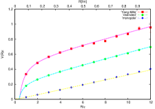
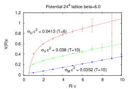
Figure 1: The static quark–antiquark potential $V(R)$ as a function of the distance $R$ in $SU(N)$ Yang-Mills theory. (from above to below): The full potential $V_{\rm full}(R)$, restricted (or “Abelian”) part $V_{\rm rest}(R)$ and magnetic–monopole part $V_{\rm mono}(R)$. (Left) $SU(2)$ at $\beta=2.5$ on $24^{4}$ lattice ⁸, (Right) $SU(3)$ at $\beta=6.0$ on $24^{4}$ lattice ⁹.

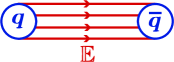
$\leftarrow$ dual $\rightarrow$  

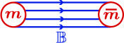
Figure 2: The electro-magnetic duality: electric charge is replaced by the magnetic charge, and the electric field is replaced by the magnetic field, and vice versa.

In order to establish the dual superconductivity, we must answer the following questions:

• How to introduce chromomagnetic monopoles in the Yang-Mills theory without scalar fields? [This should be compared with the ’t Hooft-Polyakov magnetic monopole.]

• How to define the electric-magnetic non-Abelian duality in the non-Abelian gauge theory?

• How to extract the infrared dominant mode for confinement?

In this talk,

• We give a gauge-invariant definition of (chromo)magnetic monopoles in the $SU(N)$ Yang-Mills theory (in the absence of the scalar fields) from the non-Abelian Wilson loop operator. This is achieved by using a non-Abelian Stokes theorem for the Wilson loop operator ⁶. This leads to the non-Abelian magnetic monopoles for the Wilson loop operator in the fundamental representation. This definition is independent of the gauge fixing. One does not need to use the conventional prescription called the Abelian projection proposed by ’t Hooft (1981) ⁷ which realizes magnetic monopoles by a partial gauge fixing as gauge-fixing defects.

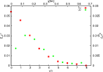
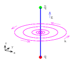
Figure 3: Ref.¹⁰: The magnetic-monopole current $\mathbf{k}$ induced around the chromoelectric flux along the $z$ axis connecting a pair of quark and antiquark. (Center panel) The positional relationship between the chromoelectric field $E_{z}$ and the magnetic current $\mathbf{k}$. (Left panel) The magnitude of the chromoelectric field $E_{z}$ and the magnetic current $J_{m}=|\mathbf{k}|$ as functions of the distance $y$ from the $z$ axis calculated from the original full variables. (Right panel) The counterparts of the left graph calculated from the restricted variables.

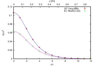
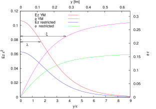
Figure 4: Ref. ¹⁰: (Left panel) The plot of the chromoelectric field $E_{z}$ versus the distance $y$ in units of the lattice spacing $\epsilon$ and the fitting as a function $E_{z}(y)$ of $y$. The red cross for the original $SU(3)$ field and the green square symbol for the restricted field. (Right panel) The order parameter $\phi$ reproduced as a function $\phi(y)$ of $y$.

In fact, the validity of this definition has been confirmed by numerical simulations on a lattice as follows.

• The magnetic monopole reproduces the linear potential with almost the same string tension $\sigma_{\rm mono}$ as the original one $\sigma_{\rm full}$: 85% for $SU(2)$ ⁸ 80% for $SU(3)$ ⁹ This is called the magnetic monopole dominance in the string tension.

• The dual Meissner effect occur in $SU(N)$ Yang–Mills theory as signaled by the simultaneous formation of the chromoelectric flux tube and the associated magnetic-monopole current induced around it. Only the component $E_{z}$ of the chromoelectric field $(E_{x},E_{y},E_{z})=(F_{14},F_{24},F_{34})$ connecting $q$ and $\bar{q}$ has non-zero value. The other components are zero consistently within the numerical errors. Therefore, the chromomagnetic field $(B_{x},B_{y},B_{z})=(F_{23},F_{31},F_{12})$ connecting $q$ and $\bar{q}$ does not exist. The magnitude of the chromoelectric field $E_{z}$ decreases quickly as the distance $y$ in the direction perpendicular to the line increases. Therefore, we have confirmed the formation of the chromoelectric flux in Yang–Mills theory on a lattice ^8,10.

• We have also shown that the restricted field $V$ reproduces the dual Meissner effect in the $SU(N)$ Yang–Mills theory on a lattice ^8,10.

The superconductor is characterized by the penetration depth $\delta$, the coherence length $\xi$, and the Ginzburg-Landau (GL) parameter $\kappa$ defined by

$$\kappa:=\frac{\delta}{\xi}\begin{cases}<\frac{1}{\sqrt{2}}&(\text{type I})\cr=\frac{1}{\sqrt{2}}&(\text{BPS})\cr>\frac{1}{\sqrt{2}}&(\text{type II})\end{cases}.$$ (1)

In the type-I superconductor, the attractive force acts between two flux tubes, while the repulsive force in the type-II superconductor. There is no interaction at $\kappa=\frac{1}{\sqrt{2}}\simeq 0.707$.

In the Abelian-Higgs model, two vortices are attractive in the type I, repulsive for the type II, and there are no force between two vortices in the BPS limit. In the Abelian case, therefore, the ordinary superconductivity must be type II or BPS. Otherwise, the initial configuration of the vortices will be eventually collapsed by the attractive force among the vortices. In fact, this is consistent with a fact that the vortices of magnetic flux tube form the Abrikosov lattice (hexagonal lattice rather than forming a square lattice) in the superconductor as stable configuration, which is verified experimentally.

In the non-Abelian case, recent numerical simulations show that the dual superconductivity of the Yang-Mills vacuum is type I, in contrast to the preceding results which claim the border between type I and type II, i.e., BPS limit.
For $SU(2)$, Kato et al.(2014) ⁸ reports the GL parameter, the penetration depth, the coherence length:

$$\kappa=0.48\pm 0.07,\ \delta=0.12{\rm fm},\ \xi=0.25{\rm fm},(m_{A}=1.64{\rm GeV},\ m_{\phi}=1.1{\rm GeV})$$ (2)

For $SU(3)$, Shibata et al.(2013) ¹⁰. reports

$$\kappa=0.45\pm 0.01,\ \delta=0.12{\rm fm},\ \xi=0.27{\rm fm},(m_{A}=1.64{\rm GeV},\ m_{\phi}=1.0{\rm GeV})$$ (3)

These results are obtained using the novel reformulation of the Yang-Mills theory, which is Cho-Duan-Ge decomposition^11-17 for $SU(2)$, and Cho-Faddeev-Niemi decomposition^18-20 for $SU(3)$.

2 Non-Abelian vortex

The type I dual superconductivity for the Yang-Mills vacuum yields the attractive force between two non-Abelian vortices. How this result is consistent with the above considerations? The crucial point is that the non-Abelian vortices have internal degrees of freedom, i.e., orientational moduli, in addition to the degrees of freedom related to the positions in space. This has a possibility for preventing the vortices from collapse due to the attractive force. Whereas the Abelian vortices have only the positions and the collapse of the lattice structure for the Abelian vortices in the type I superconductor will not be avoidable. We must examine the interaction among vortices depending on the orientational moduli in more detail. This analysis gives an estimate of the string tension based on the vortex condensation picture, and possible interactions between two non-Abelian vortices.

We discuss how the magnetic monopole condensation picture are compatible with the vortex condensation picture as another promising scenario for quark confinement. As a dual or complementary point of view, we can define a gauge-equivalent thin vortex (non-orientable) which has the magnetic monopole and the anti-magnetic monopole as the boundaries ²¹.

We want to construct the non-Abelian vortex which ends at the non-Abelian magnetic monopole, that is to say, the non-Abelian orientational zero modes of the vortex endow the endpoint non-Abelian magnetic monopole and antimonopole with same $CP^{N-1}$ zero modes.

Such a vortex will be obtained in the Higgs phase of a $U(N)$ gauge theory with $SU(N)$ flavor symmetry where the vortices with non-Abelian $CP^{N-1}$ orientational zero modes exist. This is a candidate of the dual gauge theory for describing the magnetic flux tube as a vortex solution. This is different from the dual Abelian-Higgs model with the magnetic gauge symmetry $U(1)^{N-1}$ suggested from the Abelian projection.

3 Vortex picture towards the area law

Then we discuss how such magnetic monopoles can give a nontrivial contribution to the Wilson loop operator for understanding the area law of the Wilson loop average.

The vortex condensation picture gives an easy way to understand the area law. Let us assume that the vacuum is filled with percolating thin vortices. Suppose that $N$ random vortices intersect a plane of area $L^{2}$. For simplicity, we consider the $SU(2)$ gauge group in what follows. Each intersection multiplicatively contributes a factor $(-1)^{2J}$ to the Wilson loop average and $n$ intersect within the loop take the value $(-1)^{2Jn}$. Then the probability that $n$ of the intersections occur within an area $S$ spanned by a Wilson loop is given by $(-1)^{2Jn}\left(\frac{S}{L^{2}}\right)^{n}(+1)^{N-n}\left(1-\frac{S}{L^{2}}\right)^{N-n}$.

Summing over all possibilities with the proper binomial weight yields

$$W_{C} =\sum_{n=0}^{N}\begin{pmatrix}N\\ n\end{pmatrix}(-1)^{2Jn}\left(\frac{S}{L^{2}}\right)^{n}(+1)^{N-n}\left(1-\frac{S}{L^{2}}\right)^{N-n}$$

$$=\left(1-\frac{S}{L^{2}}+(-1)^{2J}\frac{S}{L^{2}}\right)^{N}$$

$$=\left(1-\frac{[1-(-1)^{2J}]\rho S}{N}\right)^{N}\to\exp\left\{-\sigma_{J}S\right\}\quad(N\to\infty),\quad\rho:=\frac{N}{L^{2}},$$ (4)

where

$$\sigma_{J}=[1-(-1)^{2J}]\rho=\begin{cases}\sigma_{F}=2\rho&(J=\frac{1}{2},\frac{3}{2},\cdots)\cr 0&(J=1,2,\cdots)\end{cases},$$ (5)

where $L$ has been eliminated in favor of the planar vortex density $\rho:=N/L^{2}$. The limit of a large $N\to\infty$ is taken with a constant $\rho$. Thus one obtains an area law for the Wilson loop average with the string tension $\sigma_{J}$ determined by the vortex density $\rho$.

The crucial assumption in this argument is the independence of the intersection points. The asymptotic string tensions are zero for all integer-$J$ representations (with $N$-ality or “biality” being equal to $0$), while they are nonzero and equal for all half-integer $J$ representations (with $N$-ality or “biality” being equal to $1$). For the details, see Ref. ²².

4 Conclusion and discussion

1. [Magnetic monopole picture] We have given a gauge-invariant definition of the magnetic monopole in the $SU(N)$ pure Yang-Mills theory in the absence of the scalar field. This is achieved through a non-Abelian Stokes theorem for the Wilson loop operator. This enables one to estimate the magnetic monopole contribution to the Wilson loop average, which confirms the magnetic monopole dominance in the string tension. See Shibata’s talk for the numerical simulations on a lattice.

2. [Vortex picture] We have discussed the vortex solution in the Higgs phase of a gauge-Higgs model with $U(N)$ gauge fields and $N$ Higgs fields. The model fulfills the requirement that a non-Abelian vortex has the same $\bm{C}P^{N-1}$ moduli space as those of the non-Abelian magnetic monopole. The non-Abelian magnetic monopole is regarded as a kink making a junction with $N$ non-Abelian vortices with different internal orientation moduli. The internal moduli will be important to understand the type I dual superconductivity.

Acknowledgement

This work is supported by Grant-in-Aid for Scientific Research (C) 24540252 from the Japan Society for the Promotion Science (JSPS), and also in part by JSPS Grant-in-Aid for Scientific Research (S) 22224003. This work is in part supported by the Large Scale Simulation Program No.09-15 (FY2009), No.T11-15 (FY2011), No.12/13-20 (FY2012-2013) and No.13/14-23 (FY2013-2014) of High Energy Accelerator Research Organization (KEK).

References

-
[1]
Y. Nambu,
Phys. Rev. D10, 4262–4268
(1974).
G. ’t Hooft, in: High Energy Physics, edited by A. Zichichi (Editorice Compositori, Bologna, 1975).
S. Mandelstam, Phys. Report 23, 245–249 (1976). - [2] A.M. Polyakov, Phys. Lett. B59, 82–84 (1975). A.M. Polyakov, Nucl. Phys. B120, 429–458 (1977).
- [3] M.N. Chernodub, M.I. Polikarpov, [hep-th/9710205]
- [4] J. Greensite, Prog. Part. Nucl. Phys. 51, 1–83 (2003). [hep-lat/0301023]
- [5] K.-I. Kondo, S. Kato, A. Shibata and T. Shinohara, Physics Report 579, 1–226 (2015). arXiv:1409.1599 [hep-th]
- [6] K.-I. Kondo, Phys. Rev. D 77, 085029 (2008). arXiv:0801.1274 [hep-th]
- [7] G. ’t Hooft, Nucl.Phys. B190 [FS3], 455–478 (1981).
- [8] S. Kato, K.-I. Kondo, and A. Shibata, Phys. Rev. D91, 034506 (2015). arXiv:1407.2808 [hep-lat]
- [9] K.-I. Kondo, A. Shibata, T. Shinohara, and S. Kato, Phys. Rev. D83, 114016 (2011). arXiv:1007.2696 [hep-th]
- [10] A. Shibata, K.-I. Kondo, S. Kato and T. Shinohara, Phys. Rev. D87, 054011 (2013). arXiv:1212.6512 [hep-lat]
- [11] Y.S. Duan and M.L. Ge, Sinica Sci., 11, 1072–1081 (1979).
- [12] Y.M. Cho, Phys. Rev. D21, 1080–1088 (1980). Phys. Rev. D23, 2415–2426 (1981).
-
[13]
L. Faddeev and A.J. Niemi,
Phys. Rev. Lett. 82, 1624–1627
(1999).
[hep-th/9807069]
L.D. Faddeev and A.J. Niemi, Nucl. Phys. B776, 38-65 (2007). [hep-th/0608111] -
[14]
S.V. Shabanov,
Phys. Lett. B458, 322–330
(1999).
[hep-th/0608111]
S.V. Shabanov, Phys. Lett. B463, 263–272 (1999). [hep-th/9907182] - [15] K.-I. Kondo, T. Murakami and T. Shinohara, Prog. Theor. Phys. 115, 201–216 (2006). [hep-th/0504107]
- [16] K.-I. Kondo, T. Murakami and T. Shinohara, Eur. Phys. J. C42, 475–481 (2005). [hep-th/0504198]
- [17] K.-I. Kondo, Phys. Rev. D74, 125003 (2006). [hep-th/0609166]
- [18] K.-I. Kondo, T. Shinohara and T. Murakami, Prog. Theor. Phys. 120, 1–50 (2008). arXiv:0803.0176 [hep-th]
-
[19]
Y.M. Cho,
Unpublished preprint,
MPI-PAE/PTh 14/80 (1980).
Y.M. Cho, Phys. Rev. Lett. 44, 1115–1118 (1980). -
[20]
L. Faddeev and A.J. Niemi,
Phys. Lett. B449, 214–218 (1999).
[hep-th/9812090]
L. Faddeev and A.J. Niemi, Phys. Lett. B464, 90–93 (1999). [hep-th/9907180],
T.A. Bolokhov and L.D. Faddeev, Theoretical and Mathematical Physics, 139, 679–692 (2004). - [21] K.-I. Kondo, J. Phys. G: Nucl. Part. Phys. 35, 085001 (2008). arXiv:0802.3829 [hep-th]
- [22] K.-I. Kondo, T. Sasago and T. Shinohara, in preparation.