Non-equilibrium statistical mechanics of turbulence

Comments on Ruelle’s intermittency theory

Giovanni Gallavotti and Pedro Garrido

1 A hierarchical turbulence model

The proposal [8, 9] for a theory of the corrections to the OK theory (“intermittency corrections”) is to take into account that the Kolmogorov scale itsef should be regarded as a fluctuating variable.

The OK theory is implied by the assumption, for $n$ large, of zero average work due to interactions between wave components with wave length $<\kappa^{-n}\ell_{0}\equiv\ell_{n}$ and components with wave length $>\kappa\,\kappa^{-n}\ell_{0}$ ($\ell_{0}$ being the length scale where the energy is input in the fluid and $\kappa$ a scale factor to be determined) together with the assumption of independence of the distribution of the components with inverse wave length (“momentum”) in the shell $[\kappa^{n},\kappa\kappa^{n}]\ell_{0}^{-1}$, [5, p.420].

It is represented by the equalities

$$\frac{{\bf v}_{ni}^{3}}{\ell_{n}}=\frac{{\bf v}_{(n+1)i^{\prime}}^{3}}{\ell_{n+1}},\qquad{\bf v}=|v|,\ v\in R^{3}$$ (1.1)

interpreted as stating an equality up to fluctuations of the velocity components of scale $\kappa^{-n}\ell_{0}$, i.e. of the part of the velocity field which can be represented by the Fourier components in a basis of plane waves localized in boxes, labeled by $i=1,\ldots\kappa^{3n}$, of size $\kappa^{-n}\ell_{0}$ into which the fluid (moving in a container of linear size $\ell_{0}$) is imagined decomposed (a wavelet representation) so that $(n+1,i^{\prime})$ labels a box contained in the box $(n,i)$.

The length scales are supposed to be separated by a suitably large scale factor $\kappa$ (i.e. $\ell_{n}=\kappa^{-n}\ell_{0}=\kappa^{-1}\ell_{n-1}$) so that the fluctuations can be considered independent, however not so large that more than one scalar quantity (namely ${\bf v}_{n,i}^{3}$) suffices to describe the independent components of the velocity (small enough to avoid that “several different temperatures will be present among the systems $(n+1,j^{\prime})$” inside the containing box labeled $(n,j)$, and the ${\bf v}_{n+1,j}$ distribution “will not be Boltzmannian for a constant temperature inside”,[8, p.2]).

The distribution of ${\bf v}_{n+1,j}^{3}$ is then simply chosen so that the average of the ${\bf v}_{n+1,j}^{3}$ is the value ${\bf v}_{n,i}^{3}\kappa$ if the ${\bf v}_{n+1,j}^{3}$ on scale $n+1$ gives a finer description of the field in a box named $j$ contained in the box named $i$ of scale larger by one unit.

Among the distributions with this property is selected the one which maximizes entropy and is:

 

$${{}W_{ni}{\buildrel def\over{=}}|v_{ni}|^{3},\qquad\prod_{m=0}^{n}\prod_{i=1}^{\kappa^{m}}\frac{dW_{i,m+1}}{W_{i^{\prime}m}}\kappa\,e^{-\kappa\frac{W_{i,m+1}}{W_{i^{\prime},m}}}}$$

  (1.2)

with $W_{0}$ a constant that parameterizes the fixed energy input at large scale: the motion will be supposed to have a $0$ average total velocity at each point; hence $W_{0}^{\frac{1}{3}}$ can be viewed as an imposed average velocity gradient at the largest scale $\ell_{0}$.

The ${\bf v}_{in}=W^{\frac{1}{3}}_{in}$ is then interpreted as a velocity variation on a box of scale $\ell_{0}\kappa^{-n}$ or $\kappa^{-n}$ as $\ell_{0}$ will be taken $1$. The index $i$ will be often omitted as we shall mostly be concerned about a chain of boxes, one per each scale $\kappa^{-n},n=0,1,\ldots$, totally ordered by inclusion (i.e. the box labeled $(i,n)$ contains the box labeled $(i^{\prime},n+1)$).

The distribution of the energy dissipation $W_{n,i}{\buildrel def\over{=}}{\bf v}_{n,i}^{3}$ in the hierarchically arranged sequence of cells is therefore close in spirit to the hierarchical models that have been source of ideas and so much impact, at the birth of the renormalization group approach to multiscale phenomena, in quantum field theory, critical point statistical mechanics, low temperature physics, Fourier series convergence to name a few, and to their nonperturbative analysis, either phenomenological or mathematically rigorous, [10, 3, 11, 12, 2, 4, 1].

The present turbulent fluctuations model can therefore be called hierarchical model for turbulence in the inertial scales. It will be supposed to describe the velocity fluctuations at scales $n$ at which the Reynolds number is larger than $1$, i.e. as long as $\frac{{\bf v}_{n}\kappa^{-n}\ell_{0}}{\nu}>1$.

The description will of course be approximate, [9, Sec.3]: for instance the correlations of the velocity gradient components are not considered (and skewness will still rely on the classic OK theory, [7, Sec.34]).

Given the distribution (and the initial parameter $W_{0}$) it “only” remains to study its properties assuming the distribution valid for velocity profiles such that ${\bf v}_{n}\kappa^{-n}\ell_{0}>\nu$ after fixing the value of $\kappa$ in order to match data in the literature (as explained in [9, Eq.(12)]). As a first remark the scaling corrections proposed in [12] can be rederived.

The average energy dissipation in a box of scale $n$ can be defined as the average of $\varepsilon_{n}{\buildrel def\over{=}}W_{n}\ell^{-n},\,\ell_{n}=\ell_{0}\kappa^{-n}$: the latter average and its $p$”th order moments can be readily computed to be, for $p>0$:

 

$${{}\frac{\log{{\mbox{\boldmath$\langle$}}\,\varepsilon_{n}^{p}\,{\mbox{\boldmath$\rangle$}}}}{-\log\ell_{n}}\,\vtop{\halign{#\cr\rightarrowfill\crcr\kern-1.0pt\nointerlineskip\cr\hskip 3.0pt${\scriptstyle n\to\infty}$\hskip 3.0pt\crcr}}\,\tau_{p}=-\frac{\log\Gamma(1+p)}{\log\kappa},\qquad{{\mbox{\boldmath$\langle$}}\,\varepsilon_{n}^{p}\,{\mbox{\boldmath$\rangle$}}}\sim\kappa^{n\tau_{p}},}$$

  (1.3)

The $W^{\frac{1}{3}}_{n}$ being interpreted as a velocity variation on a box of scale $\ell_{0}\kappa^{-n}$, the last formula can also be read as exressing the ${{\mbox{\boldmath$\langle$}}\,(\frac{|\Delta_{r}v|}{r})^{p}\,{\mbox{\boldmath$\rangle$}}}\sim r^{\zeta_{p}}$ with $\zeta_{p}=\frac{1}{3}-\frac{\log\Gamma(\frac{p}{3}+1)}{\log\kappa}$.

The $\tau_{p}$ is the intermittency correction to the value $\frac{1}{3}$: the latter is the standard value of the OK theory in which there is no fluctuation of the dissipation per unit time and volume $\frac{W_{n}}{\ell_{n}}$; this gives us one free parameter, namely $\kappa$, to fit experimental data: its value, universal within Ruelle’s theory, turns out to be quite large, $\kappa\sim 22.75$, [8], fitting quite well all experimental $p$-values ($p<18$).

Other universal predictions are possible. In [9] a quantity has been studied for which accurate simulations are available.

If ${\bf W}$ is a sample $(W_{0},W_{1},\ldots)$ of the dissipations at scales $0,1,\ldots$ for the distribution in the hierarchical turbulence model, the smallest scale $n({\bf W})$ at which $W_{n}^{\frac{1}{3}}\ell_{0}\kappa^{-n}\simeq\nu$ occurs is the scale at which the Kolmogorv scale is attained (i.e. the Reynolds number $\frac{W_{n}^{\frac{1}{3}}\ell_{n}}{\nu}$ becomes $<1$).

Taking $\ell_{0}=1,\nu=1$, at such (random) Kolmogorov scale the actual dissipation is $\xi=W_{n({\bf W})}\kappa^{n({\bf W})}$ with a probability distribution with density $P^{*}(\xi)$. If $w_{k}=\frac{W_{k}}{W_{k-1}}$ then $W_{n}=W_{0}w_{1}\cdots w_{n}$ and the computation of $P^{*}(\xi)$ can be seen as a problem on extreme events about the value of a product of random variables. Hence is is natural that the analysis of $P^{*}$ involves the Gumbel distribution $\phi(t)$ (which appears with parameter $3$), [9].

The $P^{*}$ is a distribution (universal once the value of $\kappa$ has been fixed to fit the mentioned intermittency data) which is interesting because it can be related to a quantity studied in simulations.

It has been remarked, [9], that, assuming a symmetric distribution of the velocity increments on scale $\kappa^{-n}$ whose modulus is $W_{n,i}^{\frac{1}{3}}$, the hierarchical turbulence model can be applied to study the distribution of the velocity increments: for small velocity increments the calculation can be performed very explictly and quantitatively precise results are derived, that can be conceivably checked at least in simulations. The data analysis and the (straightfoward) numerical evaluation of the distribution $P^{*}$ is described below, following [9].

2 Data settings

Let $\ell_{0},\nu=1$ and let ${\bf W}=(W_{0},W_{1},\ldots)$ be a sample chosen with the distribution

$$p(d{\bf W})=\prod_{i=1}^{\infty}\frac{\kappa\,dW_{i}}{W_{i-1}}\,e^{-\kappa\frac{W_{i}}{W_{i-1}}}$$ (2.1)

with $W_{0},\kappa$ given parameters; and let ${\bf v}=(v_{0},v_{1},\ldots)=(W_{0}^{\frac{1}{3}},W_{1}^{\frac{1}{3}},\ldots)$.

Define $n({\bf W})=n$ as the smallest value of $i$ such that $W_{i}^{\frac{1}{3}}\kappa^{-i}\equiv v_{i}\kappa^{-i}<1$: $n({\bf W})$ will be called the “dissipation scale” of ${\bf W}$.

Imagine to have a large number ${\cal N}$ of $p$-distributed samples of ${\bf W}$’s. Given $h>0$ let

$$P_{n}^{*}(\xi){\buildrel def\over{=}}\frac{1}{h}\frac{1}{{\cal N}}\Big{(}(\#\,{\bf W}\,{\rm with}\,n({\bf W})=n)\cap(\xi<(W_{n}/W_{0})^{\frac{1}{3}}\kappa^{n}<\xi+h)\Big{)}$$ (2.2)

hence $hP^{*}_{n}(\xi)$ is the probability that the dissipation scale $n$ is reached with $\xi$ in $[\xi,\xi+h]$. Then $P^{*}(\xi){\buildrel def\over{=}}\sum_{n=0}^{\infty}P^{*}_{n}(\xi)$ is the probability density that, at the dissipation scale, the velocity gradient $\frac{v_{n}}{v_{0}}\kappa^{n}$ is between $\xi$ and $\xi+h$.

The velocity component in a direction is $v_{n}\cos\vartheta$: so that the probability that it is in $d\xi$ with gradient $\frac{v_{n}}{v_{0}}\kappa^{n}$ and that this happens at dissipation scale $=n$ is $d\xi$ times

$$\int P^{*}_{n}(\frac{v_{n}}{v_{0}}\kappa^{n}=\xi_{0})d\xi_{0}\delta(\xi_{0}|\cos\vartheta|-\xi)\frac{\sin\vartheta d\vartheta d\varphi}{4\pi}=\int_{\xi}^{\infty}\frac{P_{n}^{*}(\xi_{0})}{\xi_{0}}d\xi_{0}$$ (2.3)

Let

$$P(\xi){\buildrel def\over{=}}\int_{\xi_{0}>\xi}\frac{d\xi_{0}}{\xi_{0}}\sum_{n=1}^{\infty}P^{*}_{n}(\xi_{0})$$ (2.4)

that is the probability distribution of the (normalized radial velocity gradient) and

$$\sigma_{m}=\int_{0}^{\infty}d\xi P(\xi)\xi^{m}$$ (2.5)

its momenta. To compare this distribution to experimental data [6] it is convenient to define

$$p(z)=\frac{1}{2}\sigma_{2}^{1/2}P(\sigma_{2}^{1/2}|z|)$$ (2.6)

We have used the following computational algorithnm to $P(\xi)$:

• (1) Build a sample $(i)$ ${\bf W}^{(i)}=(W_{0},W_{1},\ldots,W_{n},\ldots)$

• (2) Stop when $n=\bar{n}_{i}$ such that $W_{n-1}^{1/3}\kappa^{-(n-1)}>1>W_{n}^{1/3}\kappa^{-n}$

• (3) Evaluate $\bar{m}_{i}=int(\xi_{i}/h)+1$ where $\xi_{i}=\kappa^{\bar{n}_{i}}(W_{\bar{n}_{i}}/W_{0})^{1/3}$

• (4) goto to (1) during $N$ times

Then, the distribution $P(\xi)$ is given by

$$P(mh-h/2)=h^{-1}\bar{P}(m)\quad,\quad\bar{P}(m)=\frac{1}{N}\sum_{i=1}^{N}\frac{1}{\bar{m}_{i}}\chi(\bar{m}_{i}\geq m)$$ (2.7)

where $\chi(A)=1$ if $A$ is true and $0$ otherwise. It is convenient to define the probability to get a given $m$ value as

$$\overline{Q}(m)=\frac{1}{N}\sum_{i=1}^{N}\delta(\bar{m}_{i},m)$$ (2.8)

where $\delta(n,m)$ is the Kronecker delta. Once obtained $\overline{Q}(m)$, we can get recursively $\bar{P}(m)$:

$$\bar{P}(m+1)=\bar{P}(m)-\frac{1}{m}\overline{Q}(m)\quad,\quad\bar{P}(1)=\sum_{m=1}^{\infty}\frac{1}{m}\overline{Q}(m)=\frac{1}{N}\sum_{i=1}^{N}\frac{1}{\bar{m}_{i}}$$ (2.9)

and the momenta distribution is then given by:

$$\sigma_{m}=h^{m}\frac{1}{N}\sum_{i=1}^{N}\frac{1}{\bar{m}_{i}}\sum_{l=1}^{\bar{m}_{i}}l^{m}$$ (2.10)

Finally, the error bars of a probability distribution (for instance $\bar{P}$) are computed by considering that the probability that in $N$ elements of a sequence there are $n$ in the box $m$ is given by the binomial distribution:

$$D_{m}(n,N)=\binom{N}{n}\bar{P}(m)^{n}\left(1-\bar{P}(m)\right)^{N-n}$$ (2.11)

From it we find

$$\langle n\rangle_{m}=N\bar{P}(m)\quad,\quad\langle(n-\langle n\rangle_{m})^{2}\rangle_{m}=\bar{P}(m)\left(1-\bar{P}(m)\right)/N$$ (2.12)

where $\langle.\rangle=\sum_{n}.D_{m}(n,N)$. Therefore, the error estimation for the $\bar{P}$ probability is given by

$$\bar{P}(m)\pm 3\left(\bar{P}(m)\left(1-\bar{P}(m)\right)/N\right)^{1/2}$$ (2.13)

We have done $15$ simulations with $\kappa=22$, $N=10^{12}$ realizations ($10^{4}$ cycles of size $10^{7}$) and different values of $W_{0}$: $10^{7}$, $10^{8}$, $5\times 10^{8}$, $10^{9}$, $2\times 10^{9}$, $3\times 10^{9}$, $4\times 10^{9}$, $5\times 10^{9}$, $10^{10}$, $2\times 10^{10}$, $5\times 10^{10}$, $7\times 10^{10}$, $10^{11}$, $2\times 10^{11}$ and $5\times 10^{11}$. We also use the Reynold’s number $R=W_{0}^{1/3}$.

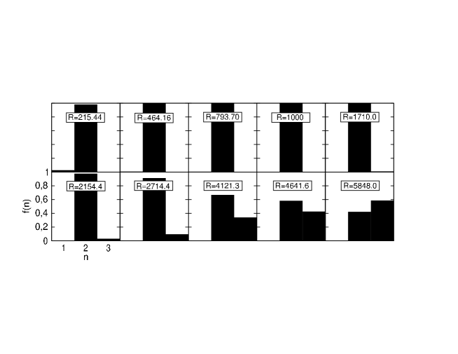
Figure 1: Distribution of events that reach the Kolmogorov scale $\kappa^{-n}$ for different values of the Reynold’s numbers $R$ and $\kappa=22$. The total number of events is $10^{12}$.

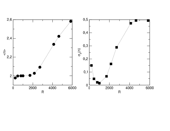
Figure 2: Momenta of the $\bar{n}$-distribution. Left: average value. Right: second momenta

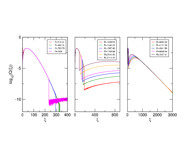
Figure 3: Plot as a function of $\xi=mh$ of the logarithm of the probability, $\log_{10}Q(\xi)$, with $Q(\xi)=\overline{Q}(\frac{\xi}{h})$, that the Kolmogorov scale is reached at scale $m=\frac{\xi}{h}$, for different Reynold’s numbers and $h=10^{-3}{{\mbox{\boldmath$\langle$}}\,\xi\,{\mbox{\boldmath$\rangle$}}}$.

Figure 4: $log_{10}p(z)$ distribution for different Reynold’s numbers. Central figure: $a(1259.92)=-0.08$, $a(1442.25)=-0.12$, $a(1587.40)=-0.24$ and $a(1709.98)=-0.52$. Right figure: $a(3684.03)=-0.51$, $a(4121.29)=-0.55$, $a(4621.59)=-0.58$, $a(5848.04)=-0.61$ and $a(7937.01)=-0.64$.

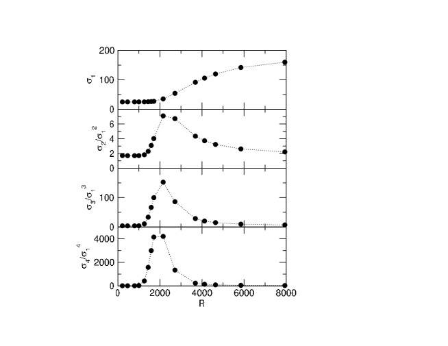
Figure 5: Measured momenta of the distribution $P(\xi)$, $\sigma_{n}$, vs Reynold’s number.

The size of $\kappa$ has been chosen to fit the data for the intermittency exponents $\zeta_{p}$ and it is quite large ($\kappa=22$, [8]): this has the consequence that the Kolmogorov scale is reached at a scale $\kappa^{-n}$ with $n=2,3$ and very seldom for higher scales, at the considered Reynolds numbers. That can be seen in Figure 1 where we show the obtained distributions of $\bar{n}_{i}$, $i=1,\ldots,N$. In Figure 2 we see the average value of $\bar{n}$ and its second momenta. We see that for low Reynold’s numbers the values is almost constant equal to $2$ and from $R\simeq 2000$ it begins to grow. The second momenta shows a minimum for $R\simeq 1000$ where almost all events are in $\bar{n}_{i}=2$.

The measured distribution of $Q(\xi)$ (see Figure 3) reflects the superposition of two distributions: the values of $\xi$ associated to the $\bar{n}_{i}=2$ and to $\bar{n}_{i}=3$ events. Moreover, for small values of $R$ the overall distribution is dominated by the events $\bar{n}_{i}=2$ and for large Reynold’s numbers it is dominated by the $\bar{n}_{i}=3$ events. At each case the form of the distribution is different: for small $R$, $log_{10}Q(\xi)$ is quadratic in $\xi$ and for large $R$ is linear in $\xi$.

The behavior of $Q$ defines the behavior of $p(z)$. In Figure 4 we see the $p(z)$ behavior. We again see clearly how for low $R$ values the distribution is non sensitive to the values of $R$ and it is Gaussian. For intermediate values of $R$ the exponential of a quadratic function is a good fit for the measured distribution and large enough values of $z$ but its parameters parameters depend on $R$. Finally for $R$ large of $3000$ the distribution changes and its behavior for large $z$ values seems to be fitted very well by a linear funcion with a $R$-depending slope.

It is interesting to show the dependence of the momenta of $\bar{P}$, $\sigma_{n}$, as a function of $R$. In Figure 5 we see their behavior. We can naturally identify three regions: Region I ($R\in[0,1000]$) where the momenta are almost constant, Region II ($R\in[1000,4000]$) where the moments grow with $R$ and Region III ($R\in[4000,\infty]$) where relative moments tend to some asymptotic value.

Figure 6: Measured $p(z)$ by Schumaher et al. [6] for different Reynold’s numbers

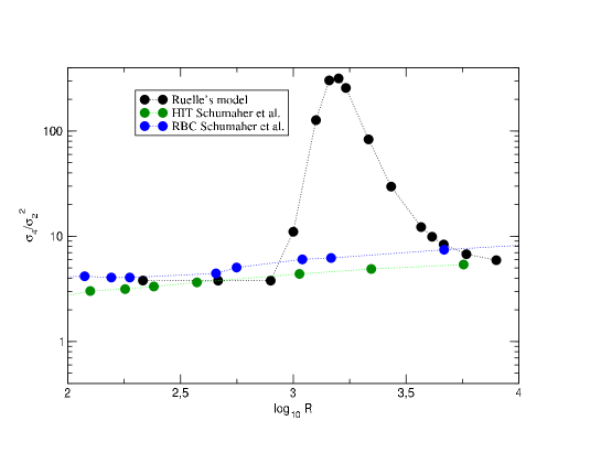
Figure 7: Measured flatness ($\sigma_{4}/\sigma_{2}^{2}$) compared with the results by Schumaher et al. [6] for different Reynold’s numbers

Experimental data can be found in [6] and are illustrated by the two plots in Figure 6 taken from the cited work

which give the function $\log_{10}p(z)$. i.e. the probability density for observing a normalized radial gradient $z$ as a function of $z=\xi/\sqrt{{{\mbox{\boldmath$\langle$}}\,\xi^{2}\,{\mbox{\boldmath$\rangle$}}}}$ in the case of homogeneous isotropic turbulence (HIT) (i.e. Navier-Stokes in a cube with periodic boundaries) or in the case of Raleigh-Benard convection (RBC) (NS+heat transport in a cylinder with hot bottom and cold top). The results of Fig. 6, for $z>0$ should be compared with those of Fig.4 at the corresponding Reynolds numbers. In both cases we see that the distribution for high Reynold numbers have linear-like behavior for large $z$-values. In fact for the HIT case and $R=2243$ we can fit a line with slope $-0.77$ in the interval $z\in[3.3,5.57]$. Also in the RBC case we can do a linear fit with slope $-0.42$ ($z\in 5.14,9.69]$) for $R=4648$. The value obtained is similar to the ones we computed on Figure 4.

In figure 7, we can compare the measured flatness in our numerical experiment with the observed by Schumaher et al. [6]. We see that the values are similar for small and large Reynold’s numbers but there is a peacked structure for intermediate values due to the relevant discontinuity when passing from $\bar{n}_{i}=2$ to $\bar{n}_{i}=3$ events.

All these results shows that the important aspect of the experiments is quite well captured with the only paramenter $\kappa$ available for the fits, i.e. a strong deviation from Gaussian behavior and the agreement of the location of the abscissae of the minima of the tails in the second case at the maximal $W_{0}$; this feature fails in the first case (HIT) as the abscissa is about $30$: is it due to a too small Reynolds number?. This seems certainly a factor to take into account as the curve appears to become independent of $R$, hence universal as it should on the basis of the theory, for $R>4000$.

In conclusion the results are compatible with the OK theory but show important deviations for large fluctuations because the Gumbel distribution does not show a Gaussian tail.

All this has a strong conceptual connotation: the basic idea (ie the proposed hierarchical and scaling distribution of the kinetic energy dissipation per unit time) is fundamental.

The need to assign a value to the scaling parameter $\kappa$ is quite interesting: in the renormalization group studies the actual value of $\kappa$ is usually not important as long as it is $\kappa>1$. Here the value of $\kappa$ is shown to be relevant (basically it appears explicitly in the end results and its value $\sim 20$ must, in principle, be fixed by comparison with simulations on fluid turbulence).

Acknowledgements: The above comments are based on numerical calculations first done by P. Garrido and confirmed by G. Gallavotti. This is the text of our comments (requested by the organizers) to the talk by D. Ruelle at the CHAOS15 conference, Institut Henri Poincaré, Paris, May 26-29, 2015.

Giovanni Gallavotti INFN-Roma1 and Rutgers University giovanni.gallavotti@roma1.infn.it Pedro Garrido Physics Dept., University of Granada garrido@onsager.ugr.es

References

- [1] G. Benfatto and G. Gallavotti. Renormalization Group. Princeton U. Press, Princeton, 1995.
- [2] P. Bleher and Y. Sinai. Investigation of the critical point in models of the type of Dyson’s hierarchical model. Communications in Mathematical Physics, 33:23–42, 1973.
- [3] F. Dyson. Existence of a phase transition in a one-dimensional Ising ferromagnet. Communications in Mathematical Physics, 12:91–107, 1969.
- [4] G. Gallavotti. On the ultraviolet stability in Statistical Mechanics and field theory. Annali di Matematica pura ed applicata, CXX:1–23, 1979.
- [5] G. Gallavotti. Foundations of Fluid Dynamics. (second printing) Springer Verlag, Berlin, 2005.
- [6] J. Schumacher and J.D. Scheel and D. Krasnov and D.A. Donzis, V. Yakhot and K.R. Sreenivasan. Small-scale universality in fluid turbulence. Proceedings of the National Academy of Sciences, 111:10961–10965, 2014.
- [7] L.D. Landau and E.M. Lifschitz. Fluid Mechanics. Pergamon, Oxford, 1987.
- [8] D. Ruelle. Hydrodynamic turbulence as a problem in nonequilibrium statistical mechanics. Proceedings of the National Academy of Science, 109:20344–20346, 2012.
- [9] D. Ruelle. Non-equilibrium statistical mechanics of turbulence. Journal of Statistical Physics, 157:205–218, 2014.
- [10] K. Wilson. Model Hamiltonians for local quantum field theory. Physical Review, 140:B445–B457, 1965.
- [11] K. Wilson. Model of coupling constant renormalization. Physical Review D, 2:1438–1472, 1970.
- [12] K. Wilson. The renormalization group. Reviews of Modern Physics, 47:773–840, 1975.