Quantum Correlations in Metals that Grow in Time and Space

Abstract

We show that the correlations of electrons with a fixed energy in metals have very anomalous time and space dependences. Due to soft modes that exist in any Fermi liquid, combined with the incomplete screening of the Coulomb interaction at finite frequencies, the correlations in 2-d systems grow with time as $t^{2}$. In the presence of disorder, the spatial correlations grow as the distance squared. Similar, but in general weaker, effects are present in 3-d systems and in the absence of quenched disorder. We propose ways to experimentally measure these anomalous correlations.

Equilibrium time-correlation functions are an essential concept in statistical mechanics Forster (1975). They describe the spontaneous fluctuations of a system in equilibrium, and together with the partition function they provide a complete description of the equilibrium state. Via the fluctuation-dissipation theorem they also describe the linear response of the system to external fields, and they are directly measurable by means of scattering experiments.

An old, and seemingly plausible, assumption is that microscopic correlations decay on time scales that are much faster than macroscopic observation times. Various concepts depend on this assumption, for instance, the notion that the BBGKY hierarchy of classical kinetic equations can be truncated Bogoliubov (1962). An analogous assumption underlies the Kadanoff-Baym scheme of deriving and solving quantum kinetic equations and its generalizations Kadanoff and Baym (1962); Langreth and Wilkins (1972). The assumption of a separation of time scales is also important in other areas, e.g., in signal processing Schwinger et al. (1998); Allen and Mills (2004). For time-correlation functions it implies that they decay exponentially for large times. Equivalently, their Laplace transform is an analytic function of the complex frequency $z$ at $z=0$. The discovery of the non-exponential decay known as long-time tails (LTTs) Alder and Wainwright (1967); Dorfman and Cohen (1970); Ernst et al. (1970), and the related breakdown of a virial expansion for transport coefficients Dorfman and Cohen (1965); Weinstock (1965) thus came as a considerable surprise Peierls (1979), since it showed that the assumption is in general not true. Rather, many time-correlation functions decay only algebraically, i.e., they have no intrinsic time scale. This scale invariance is reminiscent of the behavior of correlation functions at critical points; however, it occurs in entire phases, as opposed to just at isolated points in the phase diagram, and therefore is referred to as ‘generic scale invariance’ Nagel (1992); Dorfman et al. (1994); Belitz et al. (2005). The underlying physical reason is either conservation laws, or Goldstone modes that lead to a slow decay of some long-wavelength fluctuations and, via mode-mode-coupling effects, affect the decay of other degrees of freedom. An example is the shear stress in a classical fluid, which is not conserved, yet its time-correlation function decays algebraically as $1/t^{d/2}$ for long times $t$ in a $d$-dimensional fluid since it couples to the transverse momentum, which is conserved. As a result, the Green-Kubo expressions for various transport coefficients diverge in dimensions $d\leq 2$, and the hydrodynamic equations become nonlocal in time and space; for a review, see Ref. Belitz et al., 2005.

In classical systems in equilibrium, LTT effects, while qualitatively very important, are rather small quantitatively and become pronounced only at times so large that the correlation function is already very small overall. In non-equilibrium classical systems the effects are much more important Kirkpatrick et al. (1982); Ortiz de Zárate and Sengers (2007). In equilibrium quantum systems the corresponding effects can also be much larger, especially in systems with quenched disorder, where the quantum LTTs are often referred to as “weak-localization effects” Lee and Ramakrishnan (1985); Belitz et al. (2005). Still, the correlation functions considered to date decay as functions of time, albeit more slowly than a separation-of-time-scales argument would suggest. In this Letter we show that in a quantum system as simple as interacting electrons with no quenched disorder, i.e., the simplest model of a metal, there are correlations that not only do not decay exponentially, but actually grow with time, and in some cases also with distance. This surprising result is a consequence of generic soft, or slowly decaying, excitations in a Fermi liquid in conjunction with the incomplete screening of the Coulomb interaction at nonzero frequencies. It is a dramatic illustration of the fact that the impossibility of separating microscopic and macroscopic time scales, which is present in classical kinetics, holds a fortiori in quantum systems.

In quantum statistical mechanics it is useful to consider correlation functions that depend on one or more imaginary-time variables $\tau\in[0,1/T]$, with $T$ being the temperature, or on the corresponding imaginary Matsubara frequencies, $i\omega_{n}=2i\pi T(n+1/2)$ for fermions, and $i\Omega_{n}=2i\pi Tn$ for bosons ($n$ integer). Functions defined for imaginary Matsubara frequencies can be analytically continued to all complex frequencies, and the underlying real-time dependence can be obtained by an inverse Laplace transform. The observables in a fermion systems can be expressed in terms of expectation values of products of field operators ${\hat{\psi}}^{\dagger}({\bm{x}},\tau)$ and ${\hat{\psi}}({\bm{x}},\tau)$ that depend on the position ${\bm{x}}$ in addition to $\tau$. Spin is not essential for our purposes, and we suppress it for now. Let us consider binary products of ${\hat{\psi}}^{\dagger}$ and ${\hat{\psi}}$, and an imaginary-time Wigner operator ${\hat{W}}({\bm{X}},{\bm{x}};{\cal T},\tau)={\hat{\psi}}^{\dagger}({\bm{X}}+{\bm{x}}/2,{\cal T}+\tau/2)\,{\hat{\psi}}({\bm{X}}-{\bm{x}},{\cal T}-\tau/2)$. In a field-theoretic formulation, ${\hat{\psi}}^{\dagger}({\bm{x}},\tau)$ and ${\hat{\psi}}({\bm{x}},\tau)$ correspond one-to-one to fermionic (i.e., Grassmann-valued) fields ${\bar{\psi}}({\bm{x}},\tau)$ and $\psi({\bm{x}},\tau)$ Negele and Orland (1988), in terms of which we define a Wigner field

$$W({\bm{X}},{\bm{x}};{\cal T}\!,\tau) = {\bar{\psi}}({\bm{X}}+{\bm{x}}/2,{\cal T}+\tau/2)$$ (1)

$$\hskip 0.0pt\times\psi({\bm{X}}-{\bm{x}}/2,{\cal T}-\tau/2)$$

in analogy to the operator ${\hat{W}}$. In common applications of real-time Wigner operators or fields, ${\bm{X}}$ and $\cal T$ correspond to the “average” or “macroscopic” (presumed to be slow) length and time scale, and ${\bm{x}}$ and $\tau$ to the “relative” or “microscopic” (assumed to be fast) scales. The definition of the Wigner field reflects the assumption that it is possible and useful to separate these two scales Schwinger et al. (1998); Kadanoff and Baym (1962). In terms of it, the fluctuating particle number density is given by $n({\bm{X}},{\cal T})=W({\bm{X}},{\cal T};{\bm{x}=0},\tau=0)$, and the equilibrium single-particle Green function by $G({\bm{x}},\tau)=\langle W({\bm{X}},{\cal T};{\bm{x}},\tau)\rangle$, where $\langle\ldots\rangle$ denotes an average taken with the action governing the fermion system. If the average is taken in a non-equilibrium state, $\langle W\rangle$ also depends on ${\bm{X}}$ and ${\cal T}$. In a real-time formalism, with macroscopic time $T$ and microscopic time $t$, $\langle W({\bm{X}},{\bm{x}};T,t)\rangle=-i\,G^{<}({\bm{X}},{\bm{x}};T,t)$ is the Green function $G^{<}$ defined in Ref. Kadanoff and Baym (1962). Its Fourier transform with respect to the microscopic variables, $g^{<}({\bm{X}},T;{\bm{p}},\omega)$, is often interpreted as the density of particles with momentum ${\bm{p}}$ and energy $\omega$ at the space-time point $({\bm{X}},T)$ Kadanoff and Baym (1962); Mahan (2000). Switching back to imaginary time and frequency, this identifies

$$\rho({\bm{X}},i\omega_{n}) = T\int_{0}^{1/T}d{\cal T}\,d\tau\,e^{i\omega_{n}\tau}\,W({\bm{X}},{\cal T},{\bm{x}}=0,\tau)$$ (2)

$$= \sum_{\sigma}{\bar{\psi}}_{n,\sigma}({\bm{X}})\,\psi_{n,\sigma}({\bm{X}})$$

as the density of particles with energy $\omega_{n}$ at point ${\bm{X}}$, i.e., a spatial energy distribution. $\rho$ is related to the full phase-space distribution by summing over all momenta and averaging over the macroscopic (imaginary) time. Restoring spin, its spatial Fourier transform reads in terms of fermion fields

$$\rho({\bm{k}},i\omega_{n}) = \int d{\bm{X}}\ e^{-i{\bm{k}}\cdot{\bm{X}}}\,\rho({\bm{X}},i\omega_{n})$$ (3)

$$= \sum_{{\bm{p}},\sigma}{\bar{\psi}}_{n,\sigma}({\bm{p}}+{\bm{k}}/2)\,\psi_{n,\sigma}({\bm{p}}-{\bm{k}}/2)\ ,\qquad$$

where ${\bar{\psi}}_{n}({\bm{p}})=\sqrt{T/V}\int dx\,e^{-ipx}\,{\bar{\psi}}({\bm{x}},\tau)$ and $\psi_{n}({\bm{p}})=\sqrt{T/V}\int dx\,e^{ipx}\,\psi({\bm{x}},\tau)$, with $px={\bm{p}}\cdot{\bm{x}}-\omega_{n}\tau$, $\int dx=\int d{\bm{x}}\int_{0}^{1/T}d\tau$, and $V$ the system volume. $\rho$ depends on a macroscopic wave vector ${\bm{k}}$, but a microscopic frequency $\omega_{n}$. This is in contrast to the number density $n$, which depends on two macroscopic variables. To verify the physical interpretation of $\rho$ we note that its expectation value determines the density of states $N(\omega)$ via

$$N(\omega)=\frac{-1}{\pi}\,\frac{1}{V}\,\text{Im}\langle\rho({\bm{k}}=0,i\omega_{n}\to\omega+i0)\rangle$$ (4a)

The zeroth frequency moment gives the particle number $$N \eta=0^{+} n_{\text{F}}(\omega)$$. With the usual convergence factor Fetter and Walecka (1971) and the fermion distribution function we have

$$N=T\sum_{n}e^{i\omega_{n}\eta}\langle\rho({\bm{k}}=0,i\omega_{n})\rangle=V\int d\omega\,n_{\text{F}}(\omega)\,N(\omega)\ ,$$ (4b)

and the first frequency moment gives the energy $$E$$ carried by the particles ene ,

$$E = T\sum_{n}e^{i\omega_{n}\eta}i\omega_{n}\langle\rho({\bm{k}}=0,i\omega_{n})\rangle$$ (4c)

$$= V\int d\omega\,n_{\text{F}}(\omega)\,\omega\,N(\omega)\ .$$

Let us now consider the four-fermion correlation function $C_{\rho\rho}({\bm{X}}-{\bm{Y}};i\omega_{n},i\omega_{m})=\langle\delta\rho({\bm{X}},i\omega_{n})\,\delta\rho({\bm{Y}},i\omega_{m})\rangle$, with $\delta\rho=\rho-\langle\rho\rangle$. This is motivated by two considerations. First, in light of the above interpretation of $\rho$, $C_{\rho\rho}$ provides information about the correlations of energy levels in the Fermi system: It is the second moment of the energy density distribution. Second, the quantity $\nu({\bm{k}},i\omega_{n})=\rho({\bm{k}},i\omega_{n})-\rho({\bm{k}},-i\omega_{n})$ can be interpreted, in a technically precise sense, as an order parameter (OP) for the Fermi liquid Belitz and Kirkpatrick (2012); OP_ . $C_{\nu\nu}({\bm{k}};i\omega_{n},i\omega_{m})=\langle\delta\nu({\bm{k}},i\omega_{n})\,\delta\nu(-{\bm{k}},i\omega_{m})\rangle$ is thus the (longitudinal) OP susceptibility in an ordered phase. We will come back to this interpretation below. Writing $C_{\rho\rho}$ in imaginary-time space, and using time translational invariance, one easily sees that it consists of two distinct contributions. One piece (which one would call “disconnected” in a diagrammatic representation) is proportional to $\delta_{nm}$, and a second, “connected” one, is proportional to $T$ T_f . We focus on the connected piece by putting $\omega_{m}=-\omega_{n}$ and eliminate the trivial factor of temperature by defining

$$C({\bm{k}},i\omega_{n})=\frac{1}{VT}\,\langle\delta\rho({\bm{k}},i\omega_{n})\,\delta\rho(-{\bm{k}},-i\omega_{n})\rangle\ ,$$ (5)

which has a well-defined zero-temperature limit EPL . Since $C$ depends on a microscopic time scale, the separation-of-time-scales assumption would suggest that the analytic continuation $C({\bm{k}},i\omega_{n}\to z)$ is an analytic function of the complex frequency $z$ at $z=0$, corresponding to exponential decay in imaginary or real frequency space. From ordinary LTT physics one might expect that a coupling between the fast and slow degrees of freedom will lead instead to a nonanalytic function of the form $z^{\alpha}$, which would lead to a LTT of the form $1/t^{\alpha+1}$. We find that neither of these expectations is correct in general: In a Fermi liquid with a Coulomb interaction in $d=2$ the real-time dependence of the correlation function $C$ is

$$C({\bm{k}}\to 0,t)\propto\kappa^{2}\ln(\kappa/|{\bm{k}}|)\,t^{2}\qquad(d=2)$$ (6a)

where $$\kappa C t^{2} k L t\ll\sqrt{L\kappa}/v_{\text{F}}\kappa t v_{\text{F}} d=3$$ is the screening wave number. That is, increases with time as ; i.e., the correlations get stronger with increasing time. This behavior is cut off by a nonzero wave number or, equivalently, by a finite system size ; it is valid for times (and much larger than the microscopic time scale), with the Fermi velocity. In the behavior is a LTT,

$$C({\bm{k}}\to 0,t)\propto 1/v_{\text{F}}^{3}\,t\qquad(d=3)\ ,$$ (6b)

which is valid for $t\ll L/v_{\text{F}}$. For asymptotically large times $C$ decays exponentially, with the rate of decay going to zero as the wave number approaches zero or the system size goes to infinity.

Also of interest are the spatial correlations. For $i\omega_{n}\to 0$, i.e., for particles close to the Fermi surface, the spatial correlations decay only algebraically,

$$C({\bm{x}},i\omega_{n}\to 0)\propto\begin{cases}\sqrt{\kappa}/v_{\text{F}}^{3}\,\sqrt{r}&\qquad(d=2)\\ \kappa/v_{\text{F}}^{3}\,r^{2}&\qquad(d=3)\end{cases}$$ (7)

for distances $r=|{\bm{x}}|\gg 1/\kappa$.

These results hold for clean systems. In the presence of quenched disorder, the effects are even stronger. The time dependence in $d=2$ is the same as in the clean case and given by Eq. (6a), but in $d=3$ the correlation function does not decay with time for $t\ll L^{2}/D$,

$$C({\bm{k}}\to 0,t)\propto 1/D^{2}\,|{\bm{k}}|\qquad(d=3)\ ,$$ (8)

where $D$ is the diffusion coefficient that characterizes the diffusive electron dynamics. The spatial correlations for particles near the Fermi surface grow quadratically with the distance and remain constant in $d=2$ and $d=3$, respectively,

$$C({\bm{x}},i\omega_{n}\to 0)\propto\begin{cases}(1/D^{3})\,r^{2}&\qquad(d=2)\\ 1/D^{3}&\qquad(d=3)\ .\end{cases}$$ (9)

These expressions are again valid for distances large compared to the microscopic length. Note that for particles at the Fermi surface ($i\omega_{n}=0$) the spatial correlations at large distances in $d=3$ get cut off only by the system size. In $d=2$ they grow as the square of the distance for distances less than the localization length or the system size, whichever is smaller.

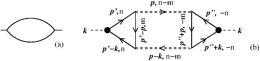
Figure 1: Diagrammatic representation of the correlation function $C({\bm{k}},i\omega_{n})$ for clean systems within (a) the effective field theory of Ref. Belitz and Kirkpatrick (2012), and (b) many-body perturbation theory. In (b), solid and double-dashed lines denote electronic Green functions and dynamically screened Coulomb potentials, respectively. Notice that no frequency is transferred at the external vertices (heavy dots); this reflects the fact that this is not a contribution to the usual density correlation function. The frequency conservation at the internal vertices is as usual.

We now sketch the origin and derivation of these surprising results, and then discuss their physical significance as well as ways to check them experimentally. We first consider clean systems. The correlation function $C$, Eq. (5), can be calculated in various ways. In the framework of the effective field theory developed in Ref. Belitz and Kirkpatrick, 2012 the leading contribution is given by the one-loop diagram shown in Fig. 1(a). The advantage of this framework is that the renormalization-group analysis of the effective theory guarantees that the result is the leading behavior; higher-loop diagrams will change the prefactor, but not the functional form of the result. Alternatively, the same result can be obtained from many-body perturbation theory Abrikosov et al. (1963) via the diagram shown in Fig. 1(b); however, there is no such guarantee within that formalism. A simplified analytical expression for either diagram, which has the correct scaling behavior, at $T\to 0$ is

$$C({\bm{k}},i\omega_{n})\propto\int_{k}^{\Lambda}dp\,p^{d-1}\int_{\omega_{n}}^{\infty}d\omega\,\frac{1}{(\omega^{2}+v_{\text{F}}^{2}p^{2})^{2}}\,\left(U(p,\omega)\right)^{2}.$$ (10)

Here $\Lambda$ is an ultraviolet momentum cutoff, and $U(p,\omega)$ is the dynamically screened Coulomb interaction. The factor of $1/(\omega^{2}+v_{\text{F}}^{2}p^{2})^{2}$ represents the soft fermionic modes. The strongly singular behavior discussed above results from a combination of the latter and the incomplete screening of the Coulomb interactions at nonzero frequencies. A short-range interaction still leads to singularities, but they are weaker than in the Coulomb case; the corresponding behavior is obtained by replacing $U(p,\omega)$ in Eq. (10) by a constant. The limit on the time regime where Eq. (6a) is valid results from the most singular behavior of $C$ in $d=2$ being restricted to frequencies $\omega_{n}$ larger than the plasma frequency. Note that the latter can be made arbitrarily small by going to small wave numbers (or to large system sizes at ${\bm{k}}=0$).

For disordered systems, an appropriate effective field theory is the generalized nonlinear sigma model that has been studied extensively in the context of metal-insulator transitions Finkelstein (1983); Belitz and Kirkpatrick (1997, 1994). The relevant one-loop diagram is still given by Fig. 1(a), but the nature of the propagators is diffusive rather than ballistic. Within the framework of many-body perturbation theory the diagram shown in Fig. 1(b) needs to be dressed with diffusion poles in elaborate ways. With any calculation method the net result is that the factor $1/(\omega^{2}+v_{\text{F}}^{2}p^{2})^{2}$ in Eq. (10) gets replaced by a diffusion pole to the fourth power, and the dynamically screened Coulomb potential gets modified to reflect the diffusive nature of the electron dynamics.

In summary, we have shown that a correlation function that describes particle-number fluctuations with a fixed energy in a Fermi liquid is a very singular function of space and time. In the zero-wave-number limit, and in a $2$-$d$ system, the correlations grow quadratically with time for times small compared to the inverse plasma frequency, and they decay only as $1/t$ in $d=3$. For particles near the Fermi surface, the correlations decay only algebraically with distance in clean systems, Eq. (7). In the presence of quenched disorder, they grow quadratically with distance in $d=2$ and remain constant in $d=3$, Eq. (9). Remarkably, this behavior is cut off only by the system size. In what follows we add some discussion remarks to put this remarkable behavior in context.

(1) As mentioned after Eq. (4c), the correlation function $C$ can be interpreted as an OP susceptibility for the Fermi liquid. An interesting analogy in this context is the corresponding OP susceptibility in a classical Heisenberg ferromagnet. Due to a coupling between the longitudinal and transverse magnetization fluctuations the longitudinal magnetic susceptibility $\chi_{\text{L}}$ (i.e., the OP susceptibility) for $2<d<4$ diverges everywhere in the ordered phase as $1/k^{4-d}$ Brézin and Wallace (1973). This results from a one-loop contribution to $\chi_{\text{L}}$ that is a wave-number convolution of two Goldstone modes, each of which scales as an inverse wave number squared. Diagrammatically this contribution has the same form as Fig. 1(a). To see the origin of the stronger effects discussed here, consider the spatial variation of $\chi_{\text{L}}$ as a function of the distance. Setting all wave-number components except for $k_{x}$ equal to zero, ${\bm{k}}=(k_{x},0,\ldots)$, we have

$$\chi_{\text{L}}(|{\bm{x}}|\to\infty)=\int dk_{x}\,e^{ik_{x}x}\,\chi_{\text{L}}(k_{x})\propto|x|^{3-d}\ .$$ (11)

That is, the correlations grow with distance for $2<d<3$. Our results for the Fermi-liquid OP susceptibility $C$ are in direct analogy to this result if one makes the following adjustments: (i) For the time or frequency dependence, replace $k_{x}$ by the frequency and put ${\bm{k}}=0$. (ii) Realize that the relevant propagator in the quantum field theory Belitz and Kirkpatrick (2012) scales as a soft mode squared, see Eq. (10). In the many-body calculation, this is apparent from the triangular fermion loops in Fig. 1(b), each of which scales as a ballistic propagator squared. (iii) Take into account the incomplete screening of the Coulomb interaction, which enhances the effect compared to the naive expectation that the quantum result should correspond to the classical one in an effective dimension $d_{\text{eff}}=d+1$.

(2) The temporal and spatial dependences of the correlation function $C$ are quite different: The underlying correlation is a function of two points in space, but four points in time; translational invariance implies that one and three of these, respectively, are independent. The time dependence of the function $C$ results from having integrated over two of the three independent time arguments, which is justified by the physical interpretation of the function $C$. A related point is that we study the behavior of $C$ for both frequency arguments approaching the Fermi surface, $\omega_{n}=-\omega_{m}\to 0$, rather than for large frequency differences. The spatial dependence of $C$, on the other hand, has the same structure as in usual two-point correlation functions. An important result is that the spatial correlations become more and more long ranged as the Fermi surface is approached.

(3) In the classical-magnet analog the strong fluctuations eventually lead to an instability of the ordered phase at the ferromagnetic transition. In the present case, this suggests the possibility of a transition from a Fermi liquid to a non-Fermi liquid with a vanishing density of states at the Fermi surface Kirkpatrick and Belitz (2012). However, whether such a transition is actually realized in any given system is a question the current theory cannot answer.

(4) We suggest two ways to experimentally observe the effects discussed here: (i) A direct measurement of the energy density distribution, e.g., in a cold-atom system, and (ii) measurements of the distribution of the local density of states, e.g., by tunneling, which is related to the correlation function $C$ as can be seen from Eq. (4a).

(5) Studies of the distribution of the local density of states in disordered metals Lerner (1988); Andreev et al. (1996) have calculated a different correlation function:, viz., the disorder average of the disconnected piece of the correlation function $C_{\nu\nu}$ defined after Eq. (4c). The effects considered were thus entirely determined by disorder fluctuations and vanish in the clean limit. In contrast, the effects considered here are caused by the electron-electron interaction, and some of them are further enhanced by disorder.

This work was supported by the NSF under grant Nos. DMR-1401410 and DMR-1401449. Part of this work was performed at the Aspen Center for Physics and supported by the NSF under grants No. PHY-10-66293.

References

- Forster (1975) D. Forster, Hydrodynamic Fluctuations, Broken Symmetry, and Correlation Functions (Benjamin, Reading, MA, 1975).
- Bogoliubov (1962) N. Bogoliubov, in Studies in Statistical Mechanics, edited by J. de Boer and G. Uhlenbeck (North-Holland, Amsterdam, 1962), vol. I.
- Kadanoff and Baym (1962) L. P. Kadanoff and G. Baym, Quantum Statistical Mechanics (W.A. Benjamin, New York, 1962).
- Langreth and Wilkins (1972) D. C. Langreth and J. W. Wilkins, Phys. Rev. B 6, 3189 (1972).
- Schwinger et al. (1998) J. Schwinger, L. L. DeRaad, Jr., K. A. Milton, and W.-Y. Tsai, Classical Electrodynamics (Westview Press, 1998).
- Allen and Mills (2004) R. L. Allen and D. W. Mills, Signal Analysis (Wiley-IEEE Press, Piscataway, NJ, 2004).
- Alder and Wainwright (1967) B. J. Alder and T. E. Wainwright, Phys. Rev. Lett. 18, 988 (1967).
- Dorfman and Cohen (1970) J. R. Dorfman and E. G. D. Cohen, Phys. Rev. Lett. 25, 1257 (1970).
- Ernst et al. (1970) M. H. Ernst, E. H. Hauge, and J. M. J. van Leeuwen, Phys. Rev. Lett. 25, 1254 (1970).
- Dorfman and Cohen (1965) J. R. Dorfman and E. G. D. Cohen, Phys. Rev. Lett. 16, 124 (1965).
- Weinstock (1965) J. Weinstock, Phys. Rev. A 140, 460 (1965).
- Peierls (1979) R. Peierls, Surprises in Theoretical Physics (Princeton University Press, 1979).
- Nagel (1992) S. Nagel, Rev. Mod. Phys. 64, 321 (1992).
- Dorfman et al. (1994) J. R. Dorfman, T. R. Kirkpatrick, and J. V. Sengers, Ann. Rev. Phys. Chem. 45, 213 (1994).
- Belitz et al. (2005) D. Belitz, T. R. Kirkpatrick, and T. Vojta, Rev. Mod. Phys. 77, 579 (2005).
- Kirkpatrick et al. (1982) T. R. Kirkpatrick, E. G. D. Cohen, and J. R. Dorfman, Phys. Rev. A 26, 995 (1982).
- Ortiz de Zárate and Sengers (2007) J. M. Ortiz de Zárate and J. V. Sengers, Hydrodynamic fluctuations in fluids and fluid mixtures (Elsevier, Amsterdam, 2007).
- Lee and Ramakrishnan (1985) P. A. Lee and T. V. Ramakrishnan, Rev. Mod. Phys. 57, 287 (1985).
- Negele and Orland (1988) J. W. Negele and H. Orland, Quantum Many-Particle Systems (Addison-Wesley, New York, 1988).
- Mahan (2000) G. D. Mahan, Many-Particle Physics (Kluwer, New York, 2000), 3rd ed., sec. 3.7.1.
- Fetter and Walecka (1971) A. L. Fetter and J. D. Walecka, Quantum Theory of Many-Particle Systems (McGraw-Hill, New York, 1971), secs. 23, 25.
- (22) More precisely, the right-hand side of Eq. (4c) equals , where and are the internal and potential energy, respectively, is the particle number, and is the chemical potential Fetter and Walecka (1971). Note that this holds for arbitrary interaction potentials between the electrons.
- Belitz and Kirkpatrick (2012) D. Belitz and T. R. Kirkpatrick, Phys. Rev. B 85, 125126 (2012).
- (24) More precisely, the OP field also depends on the “relative” momentum and equals Belitz and Kirkpatrick (2012). is thus the zeroth moment of the OP with respect to .
- (25) The disconnected piece can be written as the product of two Green functions, for the connected piece this is not possible. The factor of in the connected piece is a from the Fourier transforms of the fermion fields times a from a free imaginary-time integral. In a real-time formalism, the latter gets replaced by a free real-time integral which makes the correlation function proportional to an observation-time interval. defined in Eq. (5) has a well-defined limit given by the corresponding real-time function normalized by the observation time.
- (26) A related but different correlation function that shares some properties with the defined here has been discussed in Ref. Kirkpatrick and Belitz, 2013.
- Abrikosov et al. (1963) A. A. Abrikosov, L. P. Gorkov, and I. E. Dzyaloshinski, Methods of Quantum Field Theory in Statistical Physics (Dover, New York, 1963).
- Finkelstein (1983) A. M. Finkelstein, Zh. Eksp. Teor. Fiz. 84, 168 (1983), [Sov. Phys. JETP 57, 97 (1983)].
- Belitz and Kirkpatrick (1997) D. Belitz and T. R. Kirkpatrick, Phys. Rev. B 56, 6513 (1997).
- Belitz and Kirkpatrick (1994) D. Belitz and T. R. Kirkpatrick, Rev. Mod. Phys. 66, 261 (1994).
- Brézin and Wallace (1973) E. Brézin and D. J. Wallace, Phys. Rev. B 7, 1967 (1973).
- Kirkpatrick and Belitz (2012) T. R. Kirkpatrick and D. Belitz, Phys. Rev. Lett. 108, 086404 (2012).
- Lerner (1988) I. V. Lerner, Phys. Lett. A 133, 253 (1988).
- Andreev et al. (1996) A. Andreev, B. D. Simons, and B. L. Altshuler, J. Math. Phys. 37, 4968 (1996).
- Kirkpatrick and Belitz (2013) T. R. Kirkpatrick and D. Belitz, EPL 102, 17002 (2013).