Performance Testing of an Off-Limb Solar Adaptive Optics System

Abstract

Long-exposure spectro-polarimetry in the near-infrared is a preferred method to measure the magnetic field and other physical properties of solar prominences. In the past, it has been very difficult to observe prominences in this way with sufficient spatial resolution to fully understand their dynamical properties. Solar prominences contain highly transient structures, visible only at small spatial scales; hence they must be observed at sub-arcsecond resolution, with a high temporal cadence. An adaptive optics (AO) system capable of directly locking-on to prominence structure away from the solar limb has the potential to allow for diffraction-limited spectro-polarimetry of solar prominences. In this paper, the performance of the off-limb AO system and its expected performance, at the desired science wavelength Caii 8542 $\mathrm{\AA}$, are shown.

1 Introduction

sec:intro Solar prominences consist of relatively cool, dense plasma, which is suspended above the solar surface. Filaments and prominences represent the same phenomenon, viewed differently [Tandberg-Hanssen (1995), Labrosse et al. (2010), MacKay et al. (2010)]. The prominence itself forms within or directly beneath a magnetic flux rope [MacKay et al. (2010), Berger (2014)]. A flux rope is a long, twisted magnetic field region, which is nearly force-free [Tandberg-Hanssen (1995), MacKay et al. (2010)]. Such a flux rope may form either from the shearing of magnetic arcades, or it may emerge from below the photosphere, already formed [MacKay et al. (2010)]. One main reason that the study of solar prominence should be considered important is that they are often involved in coronal mass ejections (CMEs). CMEs occur when a flux rope becomes unstable, e.g. when there is emerging magnetic flux, coming from below [Chen (2011)]. Since flux ropes very often contain solar prominences, prominences may show instabilities that could be used to predict an imminent CME [Chen (2011)].

Despite continuing study of solar prominences, there is still much that is unknown about their physical and magnetic structure at small spatial scales [Labrosse et al. (2010), MacKay et al. (2010), Berger (2014)]. There are ambiguities related to the broadening of spectral lines of prominences that are attributed to unresolved fine structure [Labrosse et al. (2010)]. Thus the ability to measure spectra of solar prominences at very fine spatial scales is necessary to the understanding of solar prominences. Since solar prominence plasma interacts with the magnetic field in which it resides, an understanding of prominence dynamics can only be understood by the inversion of spectro-polarimetric data [MacKay et al. (2010)]. There are many ambiguities about prominence behavior, with respect to their magnetic fields, at the small spatial scales because these structures are unresolved [MacKay et al. (2010)]. Space-based instruments are capable of imaging solar prominences at very fine spatial scales [Berger et al. (2011)]. However, to the knowledge of the authors, none has been launched that can perform spectro-polarimetry on a solar prominence, which is necessary for the understanding of prominence magnetic fields [Tandberg-Hanssen (1995), MacKay et al. (2010)].

Ground-based telescopes have instruments which are capable of taking spectral and spectro-polarimetric data, for example the Interferometric BIdimensional Spectrometer (IBIS; 2006SoPh..236..415C) and the Facility Infrared Spectrometer (FIRS;2010MmSAI..81..763J) on the Dunn Solar Telescope (DST) in New Mexico. Current solar adaptive optics (AO) systems are designed to utilize broad-band light and are thus confined to locking onto structures on the disk of the Sun; prominences are invisible in broadband light [Rimmele and Marino (2011)]. This limits the usefulness of current solar AO systems. They can only be used to correct prominence images, and hence provide high resolution spectral or spectro-polarimetric data when there is a pore or other dark feature directly adjacent to the part of the limb near the prominence, as was done by 2013hsa7.conf..786O. These data, however, are fundamentally limited in resolution because AO systems can only provide their best correction extremely close to the point upon which they are locked [Hardy (1998)]. Only a purpose-built AO system that can directly lock onto solar prominence structure can allow for spectroscopic and spectro-polarimetric data at the diffraction limit of the telescope; thus allowing for an increase in humankind’s understanding of solar prominences.

The authors are the first group to construct an off-limb solar AO system mainly because of the difficulty in measuring the incoming wavefront using only light from solar prominences. The main issue is photon flux. H$\alpha$ light from solar prominences was chosen for wavefront sensor (WFS) of the off-limb solar AO system because prominences emit very brightly at this wavelength, relative to other spectral lines. Even so, the required 0.5 - 0.7 $\mathrm{\AA}$ filter bandwidth transmits very little flux. Thus, it is necessary to use all available H$\alpha$ light for the WFS. An entire AO system was designed and optimized around this WFS. The difficulty of measuring the wavefront, coupled with the need to design an entirely new AO system, is the reason why the authors are the first to build an off-limb solar AO system. (For a review of specific problems of solar AO in general, see the earlier, comprehensive reviews of 1998SPIE.3353…72R and 2011LRSP….8….2R.)

A correlating Shack-Hartmann wavefront sensor (SHWFS) was chosen for the off-limb solar AO system, due to its well known characteristics, though it is not the only type of WFS that was considered [Taylor et al. (2012)]. A standard SHWFS uses point source images directly, i.e. from a star or laser, to measure the wavefront. It does this by breaking the beam of light into small pieces, each representing a portion of the telescope aperture. The position of each star image directly corresponds to the wavefront slope at each position in the telescope aperture. A map of the wavefront is created from these slope measurements [Hardy (1998)]; see Figure pupil. Correlating SHWFS have been used in solar AO for several years [Rimmele and Radick (1998), Rimmele and Marino (2011)]. The difference between a correlating SHWFS and a conventional one is that each sub-aperture image is cross-correlated with a reference image, typically one sub-aperture image from a single frame. The maximum of each cross-correlation function shifts with the image motion, and thus the changing wavefront slope in each of the SHWFS sub-apertures [Rimmele and Radick (1998), Rimmele and Marino (2011)].

In this paper the results of some of the early tests of a closed-loop AO system on the DST are shown, based on a correlating SHWFS. In Section sec:pred, 2013SPIE.8862E..0CT is reviewed, which details the performance which was expected to be achieved from the off-limb solar AO system. In Section sec:setup, the setup of the experiment which was used to verify the performance predictions is detailed. In Section sec:res, the results of these experiment are enumerated and it is shown how they relate to the predictions in Section sec:pred.

2 Predicted Performance

sec:pred

As was stated in Section sec:intro there is very little light available for the SHWFS. Indeed, there is so little flux available, even in H$\alpha$ light, a custom made H$\alpha$ filter with very high transmission was used; see Figure fig:filter. This same type of filter will be used on the Visible Broadband Imager on the Daniel K. Inoue Solar Telescope (DKIST, formerly ATST; 2014IAUS..300..362R). A Dalsa Falcon VGA300 HG machine-vision camera was selected, due to its high sensitivity, moderate read-noise, high speed, and low cost, coupled with an in-house lenslet array, to make the SHWFS. To achieve the required speed, only a small portion of the camera chip ($160\times 160$ pixels) was read-out.

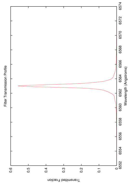
Figure 1.: Filter transmission profile of the custom H$\alpha$ filter.fig:filter

Using the high transmission filter and sensitive camera, the SHWFS is still photon starved; thus it is necessary to make trade-offs in design parameters. If the wavefront were finely sampled, by dividing the SHWFS field of view into many sub-apertures, a great deal of light would be lost and the SHWFS would no longer be able to sense the wavefront at a sufficiently high frame-rate to allow for AO correction. Therefore, fewer sub-apertures were used for this SHWFS than for the SHWFS used for on-disk observation at the DST [Rimmele and Radick (1998)]. A large field of view (FOV) per sub-aperture is also needed, to allow for the tracking of solar prominence features that are large in comparison to features seen on the disk [Taylor et al. (2012)]. Finally, the final pixel scale of the sub-aperture images must be chosen to balance resolution and image brightness [Michau, Rousset, and Fontanella (1993)]. The number of sub-apertures used, their FOV, and the final pixel scale can be determined analytically, as well as directly measured [Scharmer et al. (2003)]. To verify that an off-limb solar AO system is possible and practical, the performance of a particularly promising SHWFS configuration was modeled in detail.

2.1 WFS Noise from Indirect Methods

sec:ind It is necessary to measure the noise created by the SHWFS and to estimate noise from the various other sources that are present in a finished AO system, in order to predict the ultimate performance of an off-limb solar AO system [Hardy (1998)].

A SHWFS was setup with a $5\times 5$ array of sub-apertures (see Figure pupil), each with an FOV of $30^{\prime\prime}$ and an image scale of $0.80^{\prime\prime}$ per pixel. The image scale and FOV were measured using a resolution target. This camera was run with a frame rate of $900\mathrm{Hz}$ and exposure times of $900\mathrm{\upmu s}$. The functional form for noise generated by a correlating SHWFS is given by 2011LRSP….8….2R. However this function was explicitly stated to be defined when the Nyquist sampling criterion is satisfied, which this system cannot satisfy, due to low light levels. 1993rtpf.conf..124M give a more complete version of this formula:

$$\sigma^{2}_{x}=\frac{5m^{2}\sigma^{2}_{\mathrm{b}}}{n^{2}_{\mathrm{r}}\sigma^{2}_{\mathrm{i}}}\frac{(dp)^{2}}{(f\lambda)^{2}}\qquad[\mathrm{waves}^{2}],\ilabel{wfsn}$$ (1)

where $\sigma^{2}_{x}$ is the total noise and $m$ is the full-width at half-maximum (FWHM) of the cross-correlation (CC) peak, from the sub-aperture images (see Figure WFSIMAGE.). The quantity $\sigma^{2}_{\mathrm{b}}$ is the detector noise, which is assumed to be read-noise plus photon noise. The read noise was measured to be approximately 68 electrons per pixel (see BB, for details). The photon noise was assumed to be Poisson noise: $\sigma_{\mathrm{photon}}^{2}=g\bar{S}_{\mathrm{ADU}}$, where $g$ is the camera gain and $\bar{S}_{\mathrm{ADU}}$ is the average pixel value, in analog-to-digital units (ADUs) [Barry and Burnell (2000)]. The term $n^{2}_{\mathrm{r}}\sigma^{2}_{\mathrm{i}}$ is the energy content of the image, $d$ is the sub-aperture size, $p$ is the physical size of the pixels, $f$ is the effective focal length of the optical system (telescope plus bench optics), and $\lambda$ is the wavelength at which the measurements are made, 6563 $\mathrm{\AA}$. Note that

$$\frac{(dp)^{2}}{(f\lambda)^{2}}\approx\frac{(d\theta)^{2}}{\lambda^{2}},\ilabel{theta}$$ (2)

where $\theta$ is the image scale, in radians per pixel, and $d$ is 13.07cm (see Figure pupil).

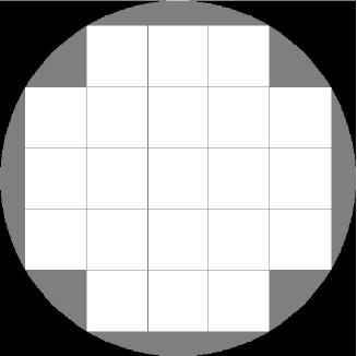
Figure 2.: The pupil layout for the $5\times 5$ grid. The outer circle is the telescope pupil, 76.2cm in diameter.pupil

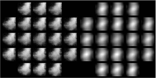
Figure 3.: SHWFS images, using the Dalsa Falcon VGA300 HG camera. On the left are prominence images which have been dark-subtracted and flat-fielded. On the right are the cross-correlation peaks.WFSIMAGE

To measure $m$, the CC peaks for the $5\times 5$ array were used [Rimmele and Marino (2011)]. Following the method of 1993rtpf.conf..124M, a two-dimensional (2D) Gaussian function was fit to the central portion of each CC peak. The value of $m$ is the average FWHM of all the CC peaks.The detector noise is again denoted as $\sigma_{\mathrm{b}}$.

The energy of the image is

$$n^{2}_{\mathrm{r}}\sigma^{2}_{\mathrm{i}}=\sum_{j}|S_{j}-\bar{S}|^{2},\ilabel{energy}$$ (3)

where $S_{j}$ and $\bar{S}$ are the signal per pixel and the average pixel value, measured in electrons [Michau, Rousset, and Fontanella (1993)].

The result of Equation (wfsn) was calculated, for each of the 2000 frames, at each exposure time, and then averaged over those 2000 frames. To make the smooth curves, as shown in Figure wfsnoise2a, one should note that 1993rtpf.conf..124M used an approximation for an image of a given contrast, using the above notation:

$$\sigma^{2}_{x}\approx\frac{5m^{2}\sigma^{2}_{\mathrm{b}}}{n^{2}_{\mathrm{r}}Cg\bar{S}_{\mathrm{ADU}}}\frac{(d\theta)^{2}}{\lambda^{2}}\qquad[\mathrm{waves}^{2}],\ilabel{wfsn2}$$ (4)

where $C$ is a factor related to the image contrast and $n^{2}_{\mathrm{r}}$ is the pixel area of each sub-aperture image. The value of $C$ is found by dividing Equation (wfsn) by Equation (wfsn2). Thus

$$C=\frac{\sigma^{2}_{\mathrm{i}}}{g\bar{S}_{\mathrm{ADU}}},\ilabel{C}$$ (5)

for an exposure time of 900$\mathrm{\upmu s}$. The results were then plotted by scaling $\sigma_{\mathrm{i}}$ and $\sigma_{\mathrm{Photon}}$ with exposure time.

2.2 WFS Error from Telemetry

sec:telem

In order to verify the above error measurements, the error in the SHWFS was found by direct measurement from SHWFS telemetry. This was done by taking the power spectrum of the total pixel shifts as measured, that is, $\mathrm{shift}=\sqrt{x_{\mathrm{shift}}^{2}+y_{\mathrm{shift}}^{2}}$. The power spectrum should be taken for data with a zero mean, as stated by marino. So the average shift was subtracted from each member of the shift array, for each data set.

Figure 4.: Noise power spectrum for data taken at 900 Hz, for moderate (top panel) and high (bottom panel) contrast prominences.pspec1

Using the method of marino, assuming white noise, we obtain

$$\sigma_{\mathrm{WFS}}^{2}=\sum_{1}^{N}{\mathrm{Noise\;level}.}\ilabel{pownoise}$$ (6)

Hhere the ’Noise level’ is the point where the power spectrum becomes flat and $N$ is the total number of exposures in each time series (see Figure pspec1). This becomes

$$\sigma_{\mathrm{WFS}}^{2}=\mathrm{Noise\;Level}\cdot N,\ilabel{pownoise2}$$ (7)

which yields the noise variance in terms of $\mathrm{pixels}^{2}$. To find the RMS noise in terms of nanometers, the following is applied,

$$\sigma_{\mathrm{WFS\;nm}}=\sigma_{\mathrm{WFS}}\theta d/(3600\cdot 57.3).\ilabel{pownoise3}$$ (8)

Here $\theta$ is the pixel scale, $0.82"$ per pixel, and $d$ is the sub-aperture diameter, 13.07 cm.

To find the error in radians, we use

$$\sigma_{\mathrm{WFS\;rad}}=2\pi\sigma_{\mathrm{WFS\;nm}}/\lambda,\ilabel{pownoise4}$$ (9)

with $\lambda$ being 6563 $\mathrm{\AA}$. The ratio between $\sigma_{\mathrm{WFS\;rad}}$ and $\sigma_{x}$, as found in Section sec:ind, was calculated for each exposure time where $\sigma_{\mathrm{WFS\;rad}}$ was defined. The value of $\sigma_{x}$ was then scaled by the average of these ratios, for each prominence. Equation (wfsn2) was then fit to the scaled $\sigma_{x}$, as shown in Figure wfsnoise2a. (The error due to the rate at which a SHWFS can measure the wavefront is also shown, as explained in Section sec:sr.) Comparing the result from Equation (wfsn) with the telemetry measurement, Equation (wfsn) is found to overestimate the noise by about a factor of 4.

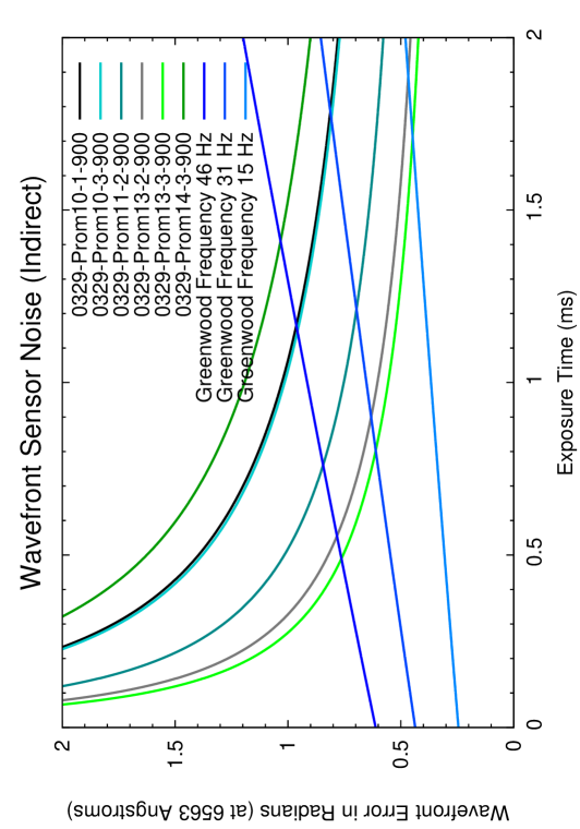
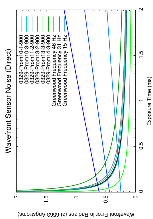
Figure 5.: Top: The solid red to green lines represent the WFS noise for the various prominences which were observed. The time delay errors (blue), are for 10cm seeing (at 5000 $\mathrm{\AA}$, 13.8 cm at 6563 $\mathrm{\AA}$, for which these errors are measured), with wind speeds of 5, 10, and 15 m s^-1, from bottom to top, respectively. These correspond to Greenwood frequencies of 15Hz, 31Hz, and 46Hz, again at H$\alpha$. See Section sec:sr for an explanation of time-delay error. Right: Noise calculated from telemetry data.wfsnoise2a

Figure wfsnoise2a shows the importance of balancing the speed of the wavefront measurements; the shorter the exposures, and thus the faster the wavefront measurements, the lower the noise from the atmosphere, but the higher the noise from the SHWFS itself. The way in which this impacts the quality of the final image in will be shown in Section sec:sr.

2.3 Strehl Ratio

sec:sr

The quality of an image is often measured in terms of its Strehl ratio. The Strehl ratio is the ratio of the intensity of the peak of a point source image measured by an imperfect optical system against the intensity of that same object as measured by a perfect optical system. A perfect optical system will have a Strehl ratio of 1. Any imperfection in the optics or caused by atmospheric distortion will lower the Strehl ratio [Hardy (1998), Born and Wolf (1999)]. A Strehl ratio above 0.8 is considered diffraction-limited [Born and Wolf (1999)]. However, an image still contains all of the information of a diffraction-limited one, only at a lower signal-to-noise ratio, until the Strehl ratio drops below about 0.1 [Hardy (1998), Lukin and Fortes (1998)]. However, the higher the achieved Strehl ratio, the higher the signal-to-noise ratio of the data.

Figure 6.: Left: Calculated Strehl ratio, taking into account all error sources. Only the curves for a Greenwood frequency of 31Hz are shown. Right: Calculated Strehl ratio from telemetry data. These data are for 8542$\mathrm{\AA}$.strehl

In order to determine the Strehl ratio that one can expect to achieve from an AO system using this SHWFS, it is necessary to account for the other primary sources of error: time delay, fitting and aliasing errors. For all of the following error estimates, a Fried parameter [Fried (1965)], $r_{0}$, of 10cm, at 5000 $\mathrm{\AA}$ was assumed (See har_98 for a more detailed discussion of AO error sources.).

To determine the error due to time delay, the functional form quoted by har_98 was used:

$$\sigma^{2}_{\mathrm{TD}}=28.4(\tau_{\mathrm{s}}f_{\mathrm{g}})^{5/3},\ilabel{td}$$ (10)

where $\tau_{\mathrm{s}}$ is the time delay, and $f_{\mathrm{g}}$ is the Greenwood frequency ($f_{\mathrm{g}}\approx 0.427\frac{v}{r_{0}}$ for a single layer atmosphere model, which was assumed for this study), $v$ being the wind speed [Hardy (1998)]. This error only takes the speed of the camera into account.

To find $\tau_{\mathrm{s}}$, the delay was assumed to be equal to the exposure time plus a constant, pessimistic 500$\upmu$s delay, for wavefront reconstruction plus the camera readout, etc. This yields $\tau_{\mathrm{s}}=500\mathrm{\upmu s+exposure\;time}$. This is similar to the method used by har_98. Three curves were calculated for $r_{0}$ of 10cm at 5000 $\mathrm{\AA}$, which is 13.8cm at 6563 $\mathrm{\AA}$, using the formula $r_{0}^{\prime}=r_{0}(\lambda/5000)^{6/5}$ [Hardy (1998)]. Wind speeds of 5, 10, and 15m s^-1 were chosen. Thus, the Greenwood frequencies were 15Hz, 31Hz, and 46Hz (see Figure wfsnoise2a). The formula for $\tau_{\mathrm{s}}$ above does not take into account the driving frequency of the deformable mirror (DM), which was unknown when this analysis was performed.

The forms of fitting and aliasing errors were used, as described by 2011LRSP….8….2R, where the fitting error is

$$\sigma^{2}_{\mathrm{F}}=0.28\left(\frac{d}{r_{0}}\right)^{5/3}.\ilabel{fit}$$ (11)

The aliasing error is

$$\sigma^{2}_{\mathrm{A}}=0.08\left(\frac{d}{r_{0}}\right)^{5/3},\ilabel{alias}$$ (12)

where $d$ is the sub-aperture size.

In Figure strehl, the resultant Strehl ratios, given the above errors, are shown. The approximation $\mathrm{Strehl\;ratio}={\mathrm{e}}^{-\sum_{i}\sigma_{i}^{2}}$ was used to find these Strehl ratios [Hardy (1998)]. All of the Strehl ratios were calculated at 8542 $\mathrm{\AA}$. To convert the SHWFS and time delay errors at 6563 $\mathrm{\AA}$, which were measured in radians, the authors took note that $1\;\mathrm{wave}=2\pi\;\mathrm{radians}$ at a given wavelength, so

$$\sigma_{8542\;\mathrm{in\;radians}}=\frac{6563}{8542}\sigma_{6563\;\mathrm{in\;radians}.}\ilabel{convert}$$ (13)

Figure strehl shows that one can expect to see Strehl ratios of between 0.6 and 0.7, at 8542 $\mathrm{\AA}$, given a Fried parameter of 10cm and 10m s^-1 wind.

There are a few important facts that can be gleaned from Figure strehl. (1) The faster the SHWFS is able to measure the wavefront, the better the achieved Strehl ratio. (2) Using faint, low contrast prominences for sensing the wavefront lowers the maximum achievable Strehl ratio. (3) For a fainter prominence, the maximum achievable Strehl ratio occurs at a slightly slower frame-rate than for a brighter prominence. (4) This SHWFS is limited by hardware to a speed of around 900Hz, which corresponds to an exposure time of about $900\upmu{\mathrm{s}}$. Given a faster camera, slightly better Strehl ratios could be achieved, but the achievable Strehl ratio decreases slowly, to the right of its maximum point.

3 Experimental Setup and Procedure

sec:setup

The off-limb AO SHWFS, as tested in Section sec:pred, was integrated into AO bench of the DST. A 97-actuator, Xinetics deformable mirror (DM) and a tilt-tip mirror (TTM) were utilized. Wavefront reconstruction is accomplished by utilizing a customized implementation of the Kiepenheuer-Institute Adaptive Optics System (KAOS), which was originally coded for the German vacuum tower telescope (VTT) and was rewritten to operate the GREGOR telescope [Berkefeld et al. (2012)]. It was customized to utilize the layout of the DM as well as the layout, exposure time, etc., of the SHWFS. This implementation of KAOS is run on an off-the-shelf computer, utilizing an Intel i7, quad-core processor. This is interfaced to the DM using a Xinetics, Gen III chassis, driving 144 channels. Of the 144 channels, 97 channels are used for the DM, 2 for the TTM, and the remaining channels are unused.

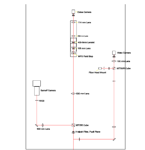
Figure 7.: The experimental setup on Port 2 of the DST. The WFS is at top, with the imaging camera at left. An interferometer can be used to verify the flatness of the DM. It is to the right of the WFS and is used by diverting all light from the WFS, via a mirror, along the rightmost red path.fig:port2-closeup

Tests were performed on Port 2 of the DST. The setup consists of a beam-splitter, which diverts 95% of the incoming H$\alpha$ light to the SHWFS, leaving the remainder to feed the imaging camera. The rest is fed to the SHWFS. The bench optics shown are required to create a $5\times 5$ SHWFS array with sub-aperture FOV of $30^{\prime\prime}$ and pixel scale of $0.82^{\prime\prime}$ per pixel (see Figure fig:port2-closeup). For these tests, the camera was run at a frame rate of $~{}860$Hz. This is slightly slower than the model frame rate, but it allowed for a border of a few pixels around the sub-aperture images ($174\times 174$ pixels are now being read-out). This allows the KAOS system to compensate for slight misalignments in the optical system. Since the system is running at a slightly slower frame rate than used in Section sec:pred, an exposure time of 1ms could be used. This lowered the noise coming from the SHWFS, at the expense of slightly more time-delay error.

3.1 Procedure

sec:proc

The KAOS system is capable of recording data which contains raw measurements from the SHWFS as well as the calculated errors in the reconstructed wavefront. KAOS records the commands sent to the TTM and the DM. It calculates the total atmospheric error in each mode, given the residual error and the commands sent to the DM. These data and their caveats are explained below.

When KAOS reconstructs the wavefront, it does so by utilizing Karhunen-Loève (K-L) modes [Noll (1976), Dai (1995)]. The degree of correction that can be achieved depends upon the number of modes that can be utilized, which in turn depends upon the resolution to which the SHWFS can sample the wavefront [Noll (1976), Hardy (1998)]. Even if those K-L modes can be perfectly determined, there is a residual error in the wavefront, corresponding to the infinite number of K-L modes which were not sensed [Noll (1976), Dai (1995)]. K-L modes are ranked in various orders. Each mode in each consecutive order contributes less to the total error in the wavefront. Thus, the correction of a few modes can correct most of the distortion in the incoming wavefront [Noll (1976), Dai (1995)]. This setup can sense 20 K-L modes. 1976JOSA…66..207N has tabulated the residual error expected after correcting 20 Zernike modes, which are similar to K-L modes, but with slightly higher residuals errors [Noll (1976), Dai (1995)].

The other major caveat is the way in which KAOS arrives at its measurements of the total wavefront error in each K-L mode. It is done by noting the residual error in each mode and determining how much correction is being applied in each mode via the TTM and the DM and combining the two. If the pixel scale of the SHWFS was measured incorrectly, both the residual and total error measurements will be wrong. However, these measurements of the pixel scale have been ensured to be accurate. The DM used was a spare at the DST, and its neutral state was not exactly flat. This coupled with any static errors in the system, which would be corrected by the DM, affects the total wavefront error measurements.

To compare the measured performance of the off-limb solar AO system with the expected performance, shown in Figure strehl, there are a few parameters which are of interest: $r_{0}$, $B_{\mathrm{cl}}$ (the closed-loop bandwidth), and the Strehl ratio of the system. If the AO loop is treated like an RC filter, where higher update frequencies are attenuated, then $B_{\mathrm{cl}}$ can be defined as the $0{\mathrm{db}}$ bandwidth. This is the highest frequency at which accurate wavefront corrections can be made [Roddier (1999)]. See the explanation of Strehl ratio in Section sec:sr.

The value of $r_{0}^{\prime}$ can be calculated from the formula given by 1976JOSA…66..207N,

$$\bar{\phi}^{2}=C\cdot(D/r_{0}^{\prime})^{5/3}.\ilabel{residual}$$ (14)

Here $D$ is the diameter of the telescope and $\bar{\phi}^{2}$ is the variance wavefront error, in radians, averaged with time. $C$ is a constant which is defined by the expected relative variance in a given mode, for a given turbulence model [Noll (1976), Dai (1995)]. The average variance of the first three K-L modes, after the two modes corresponding to tip-tilt, were used, since these have the same approximate variance of $0.023927(D/r_{0}^{\prime})^{5/3}$ [Dai (1995)]. Also, tip-tilt mode measurements are sensitive to vibrations in the room, etc. The quantity $r_{0}^{\prime}$ was calculated by finding the average wavefront error over a series of 10,000 frames, or approximately 12 s. With $r_{0}^{\prime}$ known, it is trivial to find $r_{0}$. The Strehl ratio can be approximated by[Hardy (1998)]

$${\mathrm{e}}^{-1\times[(\sum_{i}\bar{\phi}_{i}^{2})+{\mathrm{residual}}]}.\ilabel{eq:sr}$$ (15)

Here $\sum_{i}\bar{\phi}_{i}^{2}$ is the sum of the residual errors for each mode over the time series, calculated by KAOS, and the residual is approximated here as
$0.0208(D/r_{0}^{\prime})^{5/3}$ [Noll (1976)]. This is the residual for Zernike polynomials, but it is only slightly more than that for K-L modes [Noll (1976), Dai (1995)].

Finding $B_{\mathrm{cl}}$ is a bit more involved. It is found by taking the power spectrum of the residual error for a given mode with the AO system off, and plot it against the power spectrum of the same mode with the AO system on (see Figure fig:whatever). The point at which they first cross is the $0{\mathrm{db}}$ $B_{\mathrm{cl}}$. The Welch method was used to plot the power spectra [Welch (1967)].

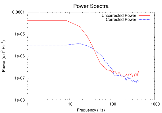
Figure 8.: The power spectra from which $B_{\mathrm{cl}}$ was calculated. The approximate $0{\mathrm{db}}$ bandwidth value was found by interpolation.fig:whatever

4 Results

sec:res

The telemetry data taken according to the procedure found in Section sec:proc were analyzed. These data were taken with the AO system correcting for 20 K-L modes. The $0{\mathrm{db}}$ bandwidth was found to be approximately $38.8$Hz (see Figure fig:whatever). This value depends upon the degree of smoothing of the power spectra, so it is only a ”ballpark figure”.

A sample of the $r_{0}$ values and Strehl ratios, which were calculated using the above method, is shown in Table tbl:results. The data represent a temporal average over a period of 12 s. One can note the large standard deviation among the $r_{0}$ values. This is due to the rapidly changing atmosphere. Since total Strehl ratio depends upon the Greenwood frequency, which was not measured with the available data, it is no surprise that there is variation in measured Strehl ratios, given similar $r_{0}$ values. Even given this fact, the below results measure favorably against the above predictions, as shown in Figure strehl. It should be noted that even with the very large values of $r_{0}$ present in some of the data sets, correction of 20 K-L modes provides higher Strehl ratios than tip-tilt correction alone. This can be seen by using Equation (residual),

$$\bar{\phi}^{2}=C\cdot(D/r_{0}^{\prime})^{5/3}.$$ (16)

If only tip-tilt errors are corrected, the constant $C$ is equal to $0.134$ [Dai (1995)]. This yields a residual error at 5000 $\mathrm{\AA}$, at $r_{0}=17.5{\mathrm{cm}}$, of $1.56$ radians². This,

$r_{0}$ cm, 5000 $\mathrm{\AA}$	Standard deviation	Strehl, 8542 $\mathrm{\AA}$	Standard deviation	Strehl, 6563 $\mathrm{\AA}$
15.9184	7.5325	0.7926	0.0652	0.6773
14.9362	6.9773	0.7884	0.0610	0.6709
17.4868	9.2392	0.8456	0.0395	0.7536
9.1684	4.7710	0.6605	0.0609	0.4978
6.4664	3.1955	0.4789	0.0713	0.2911
14.0340	6.7349	0.7797	0.0791	0.6601
12.1283	6.4545	0.7635	0.0497	0.6346
6.3531	3.2902	0.4312	0.0820	0.2457
12.4115	8.7072	0.7327	0.0707	0.5937
27.7547	16.9233	0.9097	0.0382	0.8527
46.9440	24.7305	0.9000	0.0707	0.8397
7.7688	6.6223	0.6098	0.0754	0.4366
6.5431	3.9170	0.4841	0.0989	0.3001
12.5479	6.7247	0.7827	0.0560	0.6624
13.3796	7.0181	0.7954	0.0510	0.6803
4.8167	2.5083	0.4631	0.0125	0.2716
15.0399	7.6358	0.6131	0.1380	0.4499
6.9543	3.8224	0.2626	0.1305	0.1192
5.2454	2.8631	0.1084	0.0942	0.0332
8.1936	4.3825	0.2846	0.1346	0.1349
7.2867	3.7827	0.3161	0.1220	0.1549

Table 1.: A sampling of $r_{0}$ and Strehl ratios, as calculated in Section sec:proc. The standard deviations quoted show the spread in the data over 12 s: Seeing is often quite variable.tbl:results

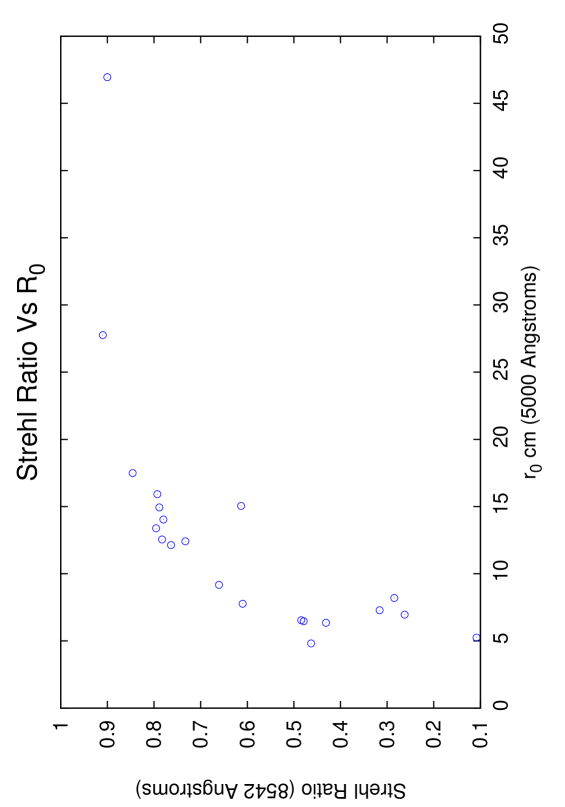
Figure 9.: A graph of Strehl ratio vs. $r_{0}$ value. This takes into account the residual wavefront errors plus the expected variance left-over from only correcting a finite number of modes (Noll, 1976). Note that for $r_{0}\approx 10$cm, the Strehl ratio is between 0.6 and 0.7, bettering the predictions in Section 2.3fig:r0

converting to radians² at 8542 $\mathrm{\AA}$, as in Equation (convert), and calculating the Strehl ratio:

$${\mathrm{Strehl\;ratio}}={\mathrm{e^{residual\;variance}}},$$ (17)

yields the maximum possible Strehl ratio at 8542 $\mathrm{\AA}$, only correcting for tip-tilt errors of $0.59$. The maximum possible Strehl ratio, given correction of 20 modes is

$0.92$ using a value of $C$ of $0.0208$ [Noll (1976)]. This system achieved $0.85$. So theoretically the improvement is small for excellent seeing, but when $r_{0}$ is $7.7$, the maximum possible Strehl ratio is $0.12$, using only tip-tilt corrections. The maximum possible Strehl ratio using 20 K-L modes is $0.72$; this system achieved an estimated Strehl ratio of $0.6$.

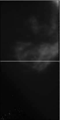
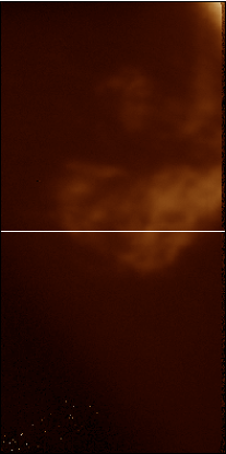
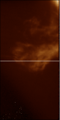
Figure 10.: The above images were taken on 10 December 2013, between 16:50 and 16:55 UTC. Each image is the average of 100 frames, with a cadence of $4s^{-1}$. Each series was taken at 6563 $\mathrm{\AA}$. They show what a long exposure would look like during moments of moderate seeing, with the AO system totally off (left), only correcting for tip-tilt errors (center), and with the AO system correcting for 20 modes. $r_{0}$ varied from between about 15cm and 17cm, when these images were taken. (The second line in Table tbl:results was taken a few moments after the right hand image was taken.) Cross sections of each image are shown by the white line. Pixel values for each will be shown in Figure fig:xsctnfig:correction

Also note that when the Strehl ratio is highest, its standard deviation is lowest, which points to the stability of the off-limb solar AO system, during times of good seeing. The 5000 $\mathrm{\AA}$ $r_{0}$ and 8542 $\mathrm{\AA}$ Strehl ratios from Table tbl:results are plotted in Figure fig:r0. Note that for $r_{0}$ around 10cm, the Strehl ratio is between 0.6 and 0.7, slightly exceeding the above predictions. This may be due to the very pessimistic time-delay error estimation. The spread in $r_{0}$ vs. Strehl ratio is almost certainly due to the variation in Greenwood frequency, but this is seen to be a secondary effect. Recall that in Section sec:proc, it was stated that there are error sources that these measurements do not take into account. Therefore, the Strehl ratios in Table tbl:results and Figure fig:r0 will almost certainly be higher than the true Strehl ratios, as might be measured at the final prominence image.

Figure 11.: Cross sections taken of each image image in Figure fig:correction. The increase in sharpness for the fully corrected image is depicted by the sharp edges shown in the graph. This indicates that much finer details are visible.fig:xsctn

Figure fig:correction depicts a few images which show the dramatic improvement that the off-limb solar AO system can provide. The images are each made from a series of 100 frames with an exposure time of 200ms each. They were taken at a frame rate of 4s^-1 and span 25s. To better show the resolution improvement made in this figure, their cross sections are plotted in Figure fig:xsctn. These images and cross sections show that even during good seeing, long integrations, which will be required for spectro-polarimetry, are vastly clearer with the off-limb solar AO system fully operating. During very bad seeing, the tip-tilt mirror can be used alone, which is still an improvement over limb tracking, the standard method for tracking prominences on the DST (Kevin Reardon, private communication).

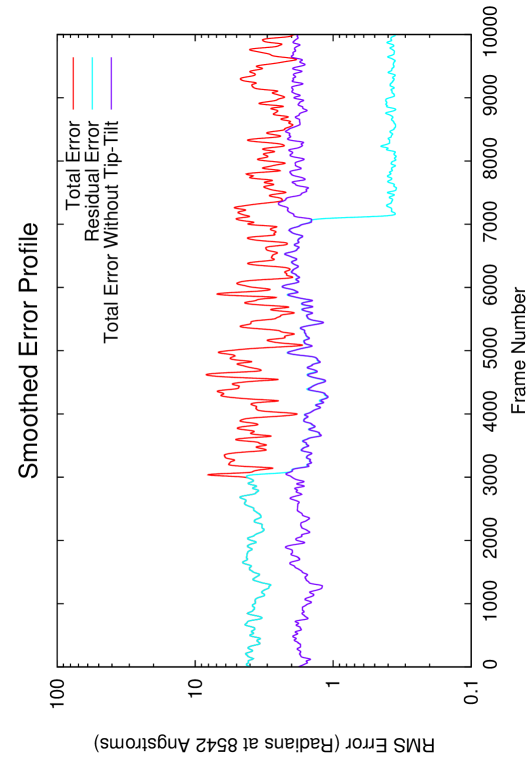
Figure 12.: Wavefront error in radians at 8542 $\mathrm{\AA}$. These data have been smoothed by convolving them with a Gaussian kernel, with a standard deviation of 15. The total error calculation becomes very noisy, once the TTM is activated, but the total, subtracting tip-tilt errors stays well behaved, even when the AO is fully activated. Since the reconstructed tip-tilt errors were not used for any calculations, this is of little consequence.fig:er1

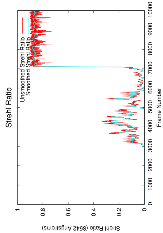
Figure 13.: Strehl ratio at 8542 $\mathrm{\AA}$ for the data plotted in Figure fig:er1. These data have been smoothed by convolving them with a Gaussian kernel, with a standard deviation of 15. Although the Strehl ratio is at times higher than 0.2, when only the TTM is active, it is highly variable.fig:st1

In Figure fig:er1, the improvement in image quality given by the off-limb solar AO system is shown. For the first 3000 frames, the AO is applying no correction, the residual error is the same as the total atmospheric error, as measured by KAOS. At around frame 3000, the system begins correcting for tip-tilt errors only. The residual error becomes the same as the total error minus the tip-tilt errors. Finally, at around frame 7000, full AO correction is applied, the residual error drops far below the total error lines. The seeing was quite good with, $r_{0}$ of around 17cm.

Figure fig:st1 Shows the corresponding Strehl ratios, calculated during the same sequence as that in Figure fig:er1. Although the seeing is good, the improvement allowed by correcting for tip-tilt errors alone is highly variable and much lower than that given by making the full correction.

5 Conclusions

The performance of the new off-limb solar AO system has been demonstrated. This system has been shown to perform well, even under less-than-ideal seeing. It performs exceedingly well during good seeing. This is the first time to the knowledge of the authors that any group has used the light of solar prominences directly to measure the wavefront in an AO system. This allows for superior correction of solar prominence images, in the near infrared, when compared to what was previously available.

The final Strehl ratio obtained by this system has been shown to exceed the predictions which was made. The Strehl ratio is high enough, under most circumstances, to allow for the reconstruction of fully diffraction-limited images, at 8542 $\mathrm{\AA}$. This allows for spectroscopy and spectro-polarimetry at the diffraction-limit of the telescope.

With the significant improvements allowed by the off-limb solar AO system, solar physicists will be able to further probe the mysteries of solar prominences, by deducing their properties at smaller spatial scales than previously possible. The authors believe that this will greatly improve humankind’s understanding of these phenomena and accompanying processes, such as CMEs.

References

- Barry and Burnell (2000) Barry, R., Burnell, J.: 2000, The Handbook of Astronomical Image Processing, Willmann-Bell, Inc., Richmond, VA.
- Berger (2014) Berger, T.: 2014, Solar prominence fine structure and dynamics. In: Schmieder, B., Malherbe, J.M., Wu, S.T. (eds.) Nature of Prominences and Their Role in Space Weather, IAU Symp. 300, 15.
- Berger et al. (2011) Berger, T., Testa, P., Hillier, A., Boerner, P., Low, B.C., Shibata, K., Schrijver, C., Tarbell, T., Title, A.: 2011, Magneto-thermal convection in solar prominences. Nature 472, 197.
- Berkefeld et al. (2012) Berkefeld , T., Schmidt, D., Soltau, D., von der Lühe, O., Heidecke, F.: 2012, The GREGOR adaptive optics system. Astron. Nachr. 333, 863.
- Born and Wolf (1999) Born, M., Wolf, E.: 1999, Principles of Optics, 7th edn. Cambridge University Press, Cambridge, UK.
- Cavallini (2006) Cavallini, F.: 2006, IBIS: A new post-focus instrument for solar imaging spectroscopy. Solar Phys. 236, 415.
- Chen (2011) Chen, P.F.: 2011, Coronal mass ejections: Models and their observational basis. Living Rev. Solar Phys. 8, (1). http://solarphysics.livingreviews.org/Articles/lrsp-2011-1/.
- Dai (1995) Dai, G.-M.: 1995, Modal compensation of atmospheric turbulence with the use of Zernike polynomials and Karhunen-Loeve functions. J. Opt. Soc. Am. 12, 2182.
- Fried (1965) Fried, D.L.: 1965, Statistics of a geometric representation of wavefront distortion. J. Opt. Soc. Am. 55, 1427.
- Hardy (1998) Hardy, J.: 1998, Adaptive Optics for Astronomical Telescopes, Oxford Univ. Press, New York.
- Jaeggli et al. (2010) Jaeggli, S.A., Lin, H., Mickey, D.L., Kuhn, J.R., Hegwer, S.L., Rimmele, T.R., Penn, M.J.: 2010, FIRS: A new instrument for photospheric and chromospheric studies at the DST. Mem. Soc. Astron. It. 81, 763.
- Labrosse et al. (2010) Labrosse, N., Heinzel, P., Vial, J.C., Kucera, T., Parenti, S., Gunár, S., Schmieder, B., Kilper, G.: 2010, Physics of solar prominences: I-Spectral diagnostics and non-LTE modelling. Space Sci. Rev. 151, 243.
- Lukin and Fortes (1998) Lukin, V.P., Fortes, B.V.: 1998, Partial correction for turbulent distortions in telescopes. Appl. Opt. 37, 4561.
- MacKay et al. (2010) MacKay, D.H., Karpen, J.T., Ballester, J.L., Schmieder, B., Aulanier, G.: 2010, Physics of solar prominences: II-Magnetic structure and dynamics. Space Sci. Rev. 151, 333.
- Marino (2007) Marino, J.: 2007, Long exposure point spread function estimation from solar adaptive optics loop data. PhD thesis. New Jersey Institute of Technology and Rutgers The State University of New Jersey - Newark.
- Michau, Rousset, and Fontanella (1993) Michau, V., Rousset, G., Fontanella, J.: 1993, Wavefront sensing from extended sources. In: Radick, R.R. (ed.) Real Time and Post Facto Solar Image Correction, Proc. 13th Sacramento Peak Summer Workshop, National Solar Observatory, 124.
- Noll (1976) Noll, R.J.: 1976, Zernike polynomials and atmospheric turbulence. J. Opt. Soc. Am. 66, 207.
- Orozco Suárez, Asensio Ramos, and Trujillo Bueno (2013) Orozco Suárez, D., Asensio Ramos, A., Trujillo Bueno, J.: 2013, Measuring vector magnetic fields in solar prominences. In: Guirado, J.C., Lara, L.M., Quilis, V., Gorgas, J. (eds.) Highlights of Spanish Astrophysics VII, Spanish Astronomical Society, 786.
- Rimmele and Marino (2011) Rimmele, T.R., Marino, J.: 2011, Solar adaptive optics. Living Rev. Solar Phys. 8, (2). http://solarphysics.livingreviews.org/Articles/lrsp-2011-2/.
- Rimmele and Radick (1998) Rimmele, T.R., Radick, R.R.: 1998, Solar adaptive optics at the National Solar Observatory. Adaptive Optical System Technologies, Proc. SPIE 3353, 72.
- Rimmele et al. (2014) Rimmele, T., Berger, T., Casini, R., Elmore, D., Kuhn, J., Lin, H., Schmidt, W., Wöger, F.: 2014, Prominence Science with ATST Instrumentation. In: Schmieder, B., Malherbe, J.M., Wu, S.T. (eds.) Nature of Prominences and Their Role in Space Weather, IAU Symp. 300, 362.
- Roddier (1999) Roddier, F. (ed.): 1999, Adaptive Optics in Astronomy, Cambridge Univ. Press, London.
- Scharmer et al. (2003) Scharmer, G.B., Dettori, P.M., Lofdahl, M.G., Shand, M.: 2003, Adaptive optics system for the new Swedish solar telescope. In: Keil, S.L., Avakyan, S.V. (eds.) Innovative Telescope and Instrumentation for Solar Astrophysics, Proc. SPIE 4853, 370.
- Tandberg-Hanssen (1995) Tandberg-Hanssen, E.: 1995, The Nature of Solar Prominences, Kluwer Academic Publishers, Dordrecht.
- Taylor et al. (2012) Taylor, G.E., Rimmele, T.R., Marino, J., Tritschler, A., McAteer, R.T.J.: 2012, Solar limb adaptive optics: A test of wavefront sensors and algorithms. In: Rimmele, T.R., Tritschler, A., Wöger, F., Collados Vera, M., Socas-Navarro, H., Schlichenmaier, R., Carlsson, M., Berger, T., Cadavid, A., Gilbert, P.R., Goode, P.R., Knölker, M. (eds.) Second ATST-EAST Meeting: Magnetic Fields from the Photosphere to the Corona., ASP Conf. Ser. 463, 321.
- Taylor et al. (2013) Taylor, G.E., Rimmele, T.R., Marino, J., McAteer, R.T.J.: 2013, An off-limb solar adaptive optics system: design and testing. In: Fineschi, S., Fennelly, J. (eds.) Solar Physics and Space Weather Instrumentation V, Proc. SPIE 88620C.
- Welch (1967) Welch, P.D.: 1967, The use of fast fourier transform for the estimation of power spectra: A method based on time averaging over short, modified periodograms. IEEE Trans. Audio Electroacoust. 15, 70.