On $m_{T}$ dependence of femtoscopy scales
for meson and baryon pairs

Abstract

The $m_{T}$-dependencies of the femto-scales, the so-called interferometry and source radii, are investigated within the hydrokinetic model for different types of particle pairs — pion-pion, kaon-kaon, proton-proton and proton-lambda, — produced in Pb+Pb and $p+p$ collisions at the LHC. In particular, such property of the femto-scales momentum behavior as $m_{T}$-scaling is studied for the systems with (w) and without (w/o) intensive transverse flow, and also w and w/o re-scattering at the final afterburner stage of the matter evolution. The detail spatiotemporal description obtained within hydrokinetic model is compared with the simple analytical results for the spectra and longitudinal interferometry radii depending on the effective temperature on the hypersurface of maximal emission, proper time of such emission, and intensity of transverse flow. The derivation of the corresponding analytical formulas and discussion about a possibility for their utilization by the experimentalists for the simple femtoscopy data analysis is the main aim of this theoretical investigation.

PACS: 24.10.Nz, 24.10.Pa, 25.75.-q, 25.75.Gz, 25.75.Ld.

Keywords: correlation femtoscopy, kaons, lead-lead collisions, proton-proton collisions, LHC.

I Introduction

The spatiotemporal structures of particle emission in nucleus-nucleus, proton-(anti)proton and proton-nucleus collisions are essentially defined by the dynamics of the collision processes Pratt ; MakSin ; Sinyuk ; Hama . Therefore the correlation interferometry Kopylov , that measures the femtoscopic scales by means of two- (or many-) particle correlations, allows one to study such processes experimentally. The corresponding femtoscopic patterns can be presented in different forms. One of them is the $k_{T}$-momentum dependence of the interferometry radii $R_{i}(k_{T}=\left|{\bf p}_{T1}+{\bf p}_{T2}\right|/2)$, that results from a 3D Gaussian fit in $q^{i}=p_{1}^{i}-p_{2}^{i}$ to the two-particle correlation function $C({\bf q},k_{T})$, defined as a ratio of the two-particle spectrum to the product of the single-particle ones. The other one is the source function $S({\bf r^{*}})$ Koonin reflecting the dependence of the pair production on the distance ${\bf r^{*}}$ between the two emitted particles in the rest frame of the pair. Both patterns supplement each other, and a reliable model should describe/predict all the mentioned types of the femtoscopic observables, if it contains a detailed space-time picture of the collision process.

It is important to note that the correlation function behavior depends also on the particle species. The detailed behavior of this dependence can be used to discriminate between different scenarios of matter evolution and particle emission in the collision processes. For example, the hydrodynamic picture of A+A collisions for the particular case of negligible transverse flow leads to the same $m_{T}^{-1/2}$ behavior of the longitudinal radii $R_{l}(k_{T})$ for the pairs of identical pions and kaons, and even leads to the complete $m_{T}$-scaling in the case of common freeze-out MakSin ; Sinyuk .

In Ref. Shap it was found that hydrokinetic model (HKM) HKM ; HKM1 ; KS ; hHKM predicts strong violation of such a scaling between pions and kaons at the LHC, and predicts $k_{T}$-scaling (for $k_{T}>k_{0}\approx 0.4$ GeV/$c$) instead. In this letter we analyze in detail the physical reasons for $m_{T}$-scaling violation. As it turned out that the reasons are quite general, there is a hope that the found $m_{T}$ peculiarities will be confirmed in the LHC experimental comparative analysis of pion and kaon femtoscopy data. In addition we predict the $m_{T}$-behavior for femtoscopic scales in other cases, including the case of meson and baryon source function radii.

To simplify the theoretical study, we reconsider the analytical results, describing $m_{T}$ (or $k_{T}$) behavior of the femtoscopy scales in a situation with strong transverse flows typical for RHIC and LHC energies. We derive a simple analytical formula for such a scenario, which fits well the complex HKM results for different hadron pairs. Since the HKM describes simultaneously the large number of bulk observables, it gives experimentalists a simple tool for estimation of the life-time of expanding fireball, related to the maximal emission of the specific hadron pair created in proton or nuclear collisions.

II Analytical model for the interferometry radii

The hydrokinetic model (HKM) (see details in Ref. hHKM ) was developed to simulate the evolution of matter formed in relativistic heavy-ion collisions and describe/predict bulk observables at RHIC and LHC. In Ref. hHKM a good description was reached for pion, kaon, (anti)proton and all charged particle spectra at different centralities, as well as for the elliptic flows. Concerning the femtoscopic scales, the confirmed HKM prediction karpsin about a reduction of $\frac{R_{out}}{R_{side}}$ ratio in A+A collisions at LHC as compared to RHIC was done; the interferometry radii for pions and kaons at RHIC hHKM ; KS and LHC hHKM ; Shap in A+A collisions were calculated; the source functions for kaons and pions at RHIC were described at the top RHIC energy and predicted for the LHC one ShapSin . In addition, HKM describes well pion interferometry radii in $p+p$ collisions at the LHC energy $\sqrt{s}=7$ TeV if one incorporates the quantum uncertainty principle into a quasi-classical event generator PBM-Sin .

All the results for A+A collisions are obtained at the same initial conditions at $\tau=0.1$ fm/$c$, produced by MC Glauber generator GLISSANDO glissando (with just re-scaled maximal initial energy density at the transition from RHIC to LHC), the same type of hydrodynamics evolution (however with different baryochemical potentials at RHIC and LHC), the same lowest temperature when the local thermal and chemical equilibrium still exist in the hydrodynamically expanding medium, $T_{ch}=165$ MeV, and with UrQMD cascade at the final afterburner stage. Such a self-consistent and reliable simulation of the data, including femtoscopy ones, indicates that the spatiotemporal picture of particle emission in the model can serve as a reference point for further studies, no matter how much advanced future models will be developed. Note, that in HKM and similar models many factors act simultaneously, the results can be obtained only by means of time-consuming numerical calculations, and it is not always clear, how each physical factor affects the complete space-time picture of the particle emission in the collision process.

Here we provide some analytical estimates for the spectra and femtoscopy scales, aiming to reveal the main parameters forming the particle emission distribution in space and time. In Refs. HKM1 ; CF the problem of spectra formation in hydrodynamic approach to A+A collisions is considered within the Boltzmann equations. It is shown analytically and illustrated by numerical calculations that the particle momentum spectra can be described by the Cooper-Frye prescription (CFp) Cooper despite freeze-out is not sharp and has the finite temporal width. The latter is equal to the inverse of the particle collision rate at 4-points ($t_{\sigma}({\bf r},p),{\bf r})$ of the maximal particle emission at a fixed momentum $p$. The set of these points forms the hypersurfaces $t_{\sigma}({\bf r},p$) which depend on the values of $p$ and typically do not enclose completely the initially dense matter. This is an important difference from the standard CFp, with a common freeze-out hypersurface (that is, typically, an isotherm) for all the momenta $p$. Also, the well known problem of CFp – negative contributions to the spectra from non-space-like parts of the freeze-out hypersurface – is naturally eliminated in this improved/generalized prescription: at each momentum $p$ the hypersurface $\sigma_{p}$ is always a space-like one.

In this letter we partially use the results of Refs. AkkSin1 ; AkkSin2 and consider the hypersurface of constant Bjorken (proper) time $\tau$, $\sigma_{p}$: $\tau=const$, as the hypersurface of maximal emission for soft enough particle momenta $p$. It is shown CF that such a hypersurface, limited in transverse direction ${\bf r}_{T}$, is typical for soft particles. For the particles with hard momenta, e. g. $p_{T}>0.8$ GeV/$c$, the hypersurface of maximal emission is different from $\tau\approx const$: there is the correlation between the transverse radius and the time of radiation (see details in AkkSin1 ; AkkSin2 ). To cut the hypersurface of maximal emission (m. e.) $\tau=\tau_{m.~{}e.}=const$ in the transverse plane for soft quanta, and at the same time get analytical approximation, we use here the Gaussian cutoff factor $\rho({\bf r}_{T})$ in the way proposed first in Refs. AkkSin1 ; AkkSin2 . Namely, the Wigner function for bosons in almost central events has the form:

$$f_{l.eq.}(x,p)=\frac{1}{(2\pi)^{3}}\left[\exp(\beta p\cdot u(\tau_{m.e.},{\bf r}_{T})-\beta\mu)-1\right]^{-1}\rho({\bf r}_{T}).$$ (1)

Here and below $\beta=1/T$ is the inverse of temperature at $\tau_{m.e.}=\sqrt{t^{2}_{m.e.}-x^{2}_{L,m.e.}}$, ${\bf r}_{T}\equiv{\bf x}_{T}$ is 2D transverse radius-vector, 4-coordinate is $x^{\mu}=(\tau\cosh\eta_{L},{\bf r}_{T},\tau\sinh\eta_{L})$ with longitudinal rapidity $\eta_{L}=\text{arctanh}\,v_{L}=\frac{1}{2}\ln\frac{t+x_{L}}{t-x_{L}}$, transverse rapidity $\eta_{T}\equiv\eta_{T}(r_{T})=\text{arctanh}\,v_{T}(r_{T})$, the hydrodynamic velocity $u^{\mu}(x)=(\cosh\eta_{L}\cosh\eta_{T},\frac{{\bf r}_{T}}{r_{T}}\sinh\eta_{T},\sinh\eta_{L}\cosh\eta_{T})$. The cutoff factor $\rho({\bf r}_{T})$ has the form AkkSin1 ; AkkSin2 :

$$\rho({\bf r}_{T})=\exp[-\alpha(\cosh\eta_{T}(r_{T})-1)].$$ (2)

Here, according to results of AkkSin1 ; AkkSin2 and the interpretation corrected for the improved CFp CF , the parameter $\alpha=R_{v}^{2}/R_{T}^{2}$, where $R_{T}$ is the transverse homogeneity length in $r_{T}$ (near $r_{T}=0$ for small $k_{T}$ ) along the hypersurface $\tau=\tau_{m.e.}=const$, and $R_{v}$ is the hydrodynamic length, $R_{v}=(v^{\prime}(r_{T}))^{-1}$, near the same $r_{T}$. The small $\alpha$ can be reached at very intensive flow when the hydrodynamic length $R_{v}$ is much smaller than the homogeneity length $R_{T}$ (which is, generally speaking, different for different particles), while the upper limit is reached in the case of no transverse flow, $R_{v}=\infty$. One can see that the contributions from particles with high momenta emitted from the hypersurface $\tau=\tau_{m.e.}=const$ are suppressed by the cutoff factor, since such particles radiate typically from rapidly moving fluid elements, $\cosh\eta_{T}(r_{T})\gg 1$. Another $\tau({\bf r}_{T})$ hypersurface should be used for hard particles.

To get single particle spectra $p_{0}d^{3}N/d^{3}p$ and the correlation function of bosons $C(p,q)$ in smoothness & mass shell approximation, we use the generalized Cooper-Frye method as it was discussed above:

$$p_{0}\frac{d^{3}N}{d^{3}p}=\int_{\sigma_{m.e.}(p)}d\sigma_{\mu}p^{\mu}f_{l.eq.}(x,p),$$ (3)

$$C(p,q)\approx 1+\frac{\left|\int_{\sigma_{m.e.}(k)}d\sigma_{\mu}k^{\mu}f_{l.eq.}(x,k)\exp(iqx)\right|^{2}}{\left(\int_{\sigma_{m.e.}(k)}d\sigma_{\mu}k^{\mu}f_{l.eq.}(x,k)\right)^{2}},$$ (4)

where $q=p_{1}-p_{2}$, $k^{\mu}=(\sqrt{m^{2}+\left(\frac{\mathbf{p_{1}}+\mathbf{p_{2}}}{2}\right)^{2}},\frac{\mathbf{p_{1}}+\mathbf{p_{2}}}{2})$. Note that in smoothness & mass shell approximation $k\approx p=(p_{1}+p_{2})/2$. Then 4-vector $q$ has three independent components, which can be selected along the beam axis, $q_{long}\equiv q_{l}$, along the pair transverse momentum vector ${\bf k}_{T}$, $q_{out}\equiv q_{o}$, and along side direction, $q_{side}\equiv q_{s}$, being orthogonal to both long and out directions.

With all these notations, one can apply the saddle point method (in complex plane) to calculate the spectra and correlation function (4) in Boltzmann approximation for longitudinally boost-invariant expansion. The results were obtained in Ref. Tolstykh on the base of the approach using the Wigner function (1) AkkSin1 ; AkkSin2 . The remarkable fact is that the behavior of the correlation function in long direction depends solely on the parameter $\alpha$ and does not depend on the transverse velocity profile at the hypersurface of maximal emission, while, as expected, the behavior of the correlation function in out and side directions is model dependent and quite sensitive to the details of the velocity profile. Because of this, here we analyze and use only the longitudinal projection of the correlation function. Let us introduce the value $\lambda$, associated with the homogeneity length in longitudinal direction in a presence of transverse flow $\lambda_{l}=\tau\sqrt{\frac{T}{m_{T}}(1-\bar{v}^{2}_{T})^{1/2}}$ AkkSin1 ; AkkSin2 :

$$\lambda^{2}=\frac{\lambda_{l}^{2}}{\tau^{2}}=\frac{T}{m_{T}}(1-\bar{v}^{2}_{T})^{1/2},$$ (5)

where the transverse velocity in the saddle point $\bar{v}_{T}=k_{T}/(m_{T}+\alpha T)$. Here $T=T_{m.e.}$ is the temperature at the hypersurface of maximal emission, $\tau=\tau_{m.e.}$. Then in LCMS Tolstykh :

$$C(k,q_{l},q_{s}=q_{o}=0)=1+\frac{\exp\left[\frac{2}{\lambda^{2}}\left(1-\sqrt{1+\tau^{2}\lambda^{4}q_{l}^{2}}\right)\right]}{\left[1+\tau^{2}\lambda^{4}q_{l}^{2}\right]^{3/2}}\stackrel{{\scriptstyle k_{T}\rightarrow\infty}}{{\longrightarrow}}1+\exp(-\lambda_{l}^{2}q_{l}^{2}).$$ (6)

At large $m_{T}/T\gg 1$ the correlation function has the Gaussian form, the interferometry radii coincide with homogeneity lengths in this approximation, that was first obtained for pure Bjorken expansion (without transverse flow: $\bar{v}_{T}=0$) in Ref. MakSin : $R_{l}=\lambda_{l}=\tau\sqrt{\frac{T}{m_{T}}}$. In Ref. Bertsch for the same case (no transverse flow) there was found the correction to the interferometry radii at small ratio $m_{T}/T\approx 1$, that can be actual for pions:

$$R_{l}^{2}=\lambda_{l}^{2}\rightarrow\lambda_{l}^{2}\frac{K_{2}(\frac{m_{T}}{T})}{K_{1}(\frac{m_{T}}{T})},$$ (7)

where $K_{n}$ are modified Bessel functions. As one can see from (6), at not large $m_{T}/T\approx 1$ the correlation function has non-Gaussian form in $q_{l}$. Correspondingly, at not large $m_{T}/T$ such a radius describes only the peak of the correlation function, where the Gaussian approximation in the limit of small $q_{l}$, $C(q_{l})=1+\exp({-R_{l}^{2}q_{l}^{2})}$, can be obtained. The detail analysis of different analytical approximations for interferometry radii is done in Ref. Tolstykh .

The approximation of the correlation function (6) at small $q_{l}$ leads to the following analytical result for the interferometry radii in the case of boost-invariant longitudinal expansion and transverse flow with arbitrary velocity profile:

$$R^{2}_{l}(k_{T})=\tau^{2}\lambda^{2}\left(1+\frac{3}{2}\lambda^{2}\right).$$ (8)

The $\lambda$ is defined by the formula (5). The direct comparison with the formula (7) for pure Bjorken picture (in our case it corresponds to $\alpha\rightarrow\infty$) demonstrates only $1-3\%$ deviation between the two results in all actual $k_{T}$ interval for pions. An advantage of the formula (8) is that it is derived for the case of transverse flow of any intensity that is especially important for LHC energies.

III Analytic fitting of HKM results

The idea of $m_{T}$-scaling for the interferometry radii of different bosons has been launched by the 1D hydrodynamic result MakSin : $R_{l}\propto\sqrt{T/m_{T}}$. The formulas (7) and (8) extended for all $m_{T}$ values in the case of 1D expansion (it means $\alpha=\infty\Rightarrow\bar{v}_{T}=0$ in f-la (8)) also lead to scaling: $R_{l}$ is the function of $\tau$ and $m_{T}/T$ only. In Fig. 1 we demonstrate the corresponding fit to the HKM results for pions and kaons with the standard Cooper-Frye prescription at the “freeze-out” hypersurface $T=165$ MeV, where we artificially switched off the UrQMD re-scattering, leaving only resonance decays. As we see, the best fits are very bad: $\chi^{2}/\text{ndf}=2562.31$ for pions and $\chi^{2}/\text{ndf}=585.24$ for kaons, and there is no $m_{T}$-scaling. The absence of $m_{T}$ scaling in full HKM (with re-scattering at the afterburner UrQMD stage) for $R_{l}$ at LHC energies is noticed recently in Ref. Shap .

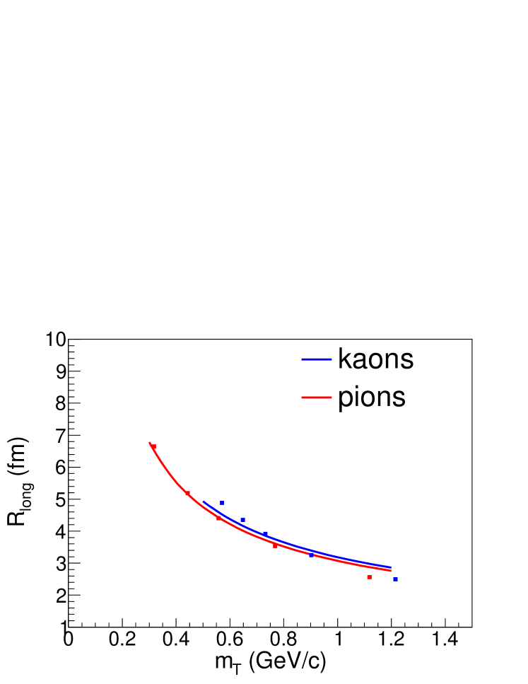
Figure 1: The $m_{T}$ dependencies of longitudinal femtoscopy radius $R_{l}$ calculated in HKM model without re-scattering stage for $K^{ch}K^{ch}$ and $\pi^{-}\pi^{-}$ pairs (markers) together with the corresponding fits (lines) according to formula (8) where transverse flow is absent ($\alpha=\infty$). The temperature is $T=165$ MeV. The results are related to $\sqrt{s_{NN}}=2.76$ GeV Pb+Pb collisions at the LHC, $c=0-5\%$, $|\eta|<0.8$, $0.14<p_{T}<1.5$ GeV/$c$.

One of the reasons for violation of scaling in HKM becomes clear from Fig. 2 where the same results of “succise” HKM (without re-scattering) were fitted by the full f-la (8) that accounts for transverse flow. Here we also use the “freeze-out” temperature 165 MeV. The fits for both pions and kaons are quite satisfactory with the same value of temperature parameter and times $\tau_{\pi}=7.41$ fm/$c$ for pions and $\tau_{K}=7.56$ fm/$c$ for kaons. For both mesons $\alpha=2.8$. These fits illustrate that, as one can see from (8), (5), the transverse flow destroys $m_{T}$ scaling, since the interferometry radius depends now on both variables $m_{T}/T$ and $k_{T}/T$.

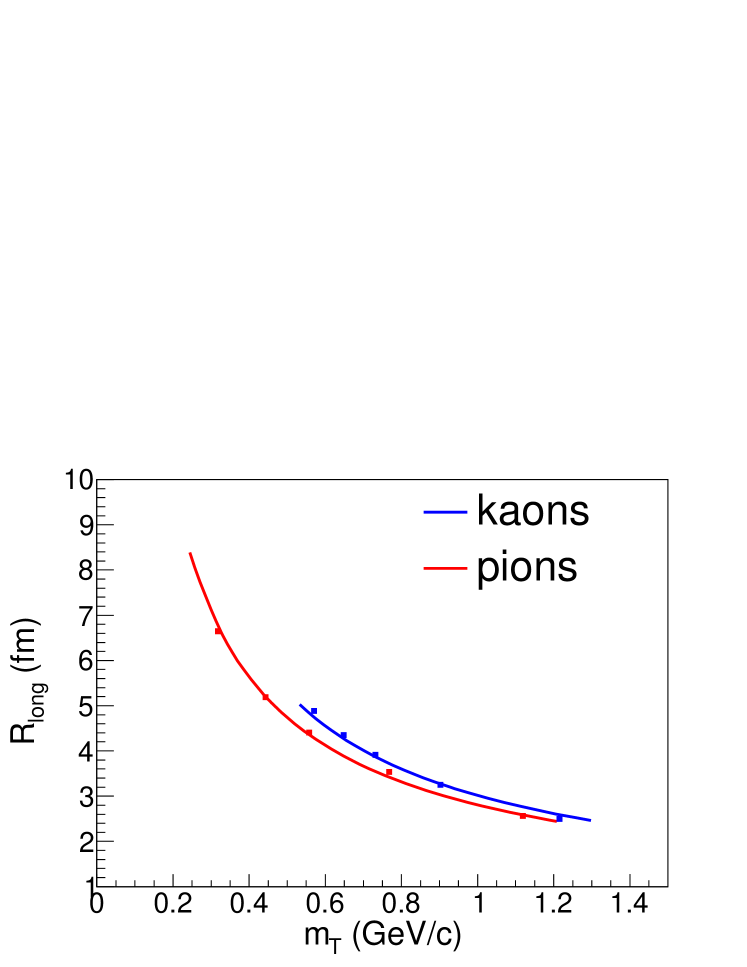
Figure 2: The same as in Fig. 1 but fits account now for the intensive transverse flow, $\alpha=2.8$. The time parameters for pions and kaons are $\tau_{\pi}=7.41$ fm/$c$ and $\tau_{K}=7.56$ fm/$c$ correspondingly, $T_{\pi}=T_{K}=165$ MeV.

The additional reason for $m_{T}$-scaling violation could be re-scattering at the afterburner stage that also can break the similarity between pion and kaon longitudinal interferometry radii. A non-Gaussian shape of the correlation functions also affects the $m_{T}$-behavior of the corresponding femtoscopy scale. To investigate in detail the role of these factors, we should analyze the results of full HKM calculation (including the re-scattering stage). In order to define the effective $T$ and $\alpha$ parameter values for an analysis of the interferometry radii behavior in full HKM, one can study the corresponding momentum spectra. These parameters can be extracted from the combined fit to pion and kaon spectra calculated in HKM, accounting for transverse flow. Such a fit can be performed using the formula obtained in the same approximation as the result (6) AkkSin2 :

$$p_{0}\frac{d^{3}N}{d^{3}p}\propto\exp{[-(m_{T}/T+\alpha)(1-\bar{v}^{2}_{T})^{1/2}]}.$$ (9)

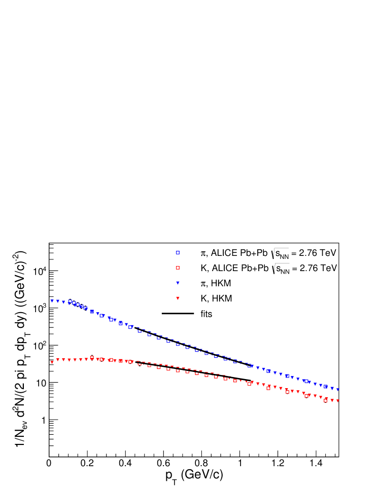
Figure 3: Pion (blue) and kaon (red) momentum spectra in Pb+Pb collisions at the LHC, $\sqrt{s_{NN}}=2.76$ GeV. Open squares show experimental values AliceSpec , triangles show HKM results, black lines correspond to combined (with the same temperature $T$) pion and kaon spectra fit according to (9).

In Fig. 3 one can see the experimental AliceSpec and HKM spectra together with the combined pion-kaon fit to HKM points. The fit with a common temperature is performed according to (9) in $p_{T}$-range $0.5-1.0$ GeV/$c$. The extracted parameter values are the following: $T=144\pm 3$ MeV, $\alpha_{\pi}=5.0\pm 3.5$ and $\alpha_{K}=2.2\pm 0.7$. To maximally reduce the effect of the non-Gaussian correlation functions, we restrict the fitting range to $q=0-0.04$ GeV/$c$ when extracting the interferometry radii from full HKM. One can see the $m_{T}$-dependence of the radii extracted in such a way in Fig. 5 together with the analytical fit according to Eq. (8), where $T$, $\alpha$ are constrained according to the combined spectra fit. The maximal emission times extracted from the fit for pions and kaons are $\tau_{\pi}=9.44\pm 0.02$ fm/$c$ and $\tau_{K}=12.40\pm 0.04$ fm/$c$ respectively while the rest of parameters take values $T_{\pi}=147$ MeV, $T_{K}=141$ MeV, $\alpha_{\pi}=8.5$ and $\alpha_{K}=1.5$. For comparison, let us present the pion and kaon emission pictures in HKM based on the invariant emission functions $G(x,p)=p^{0}\frac{d^{7}N}{d^{4}xd^{3}p}$. In Fig. 4, we demonstrate the reduced emission function averaged over all momentum angles $g(r_{T},\tau;p_{T})=\left.\frac{p^{0}d^{6}N}{dr_{o}dr_{s}d\eta d\tau dp_{T}dy}\right|_{r_{s}=0}$ for pions and kaons at $0.2<p_{T}<0.3$ Gev/$c$ in the central rapidity bins for both space-time $\eta$ and momentum $y$ rapidities. Here $r_{o}$ is the component of ${\bf r}_{T}$ along the vector ${\bf p}_{T}$, and $r_{s}$ is its component in the transverse direction orthogonal to ${\bf p}_{T}$. Such a type of the emission function (in $r_{s}$ and $r_{o}$ variables) was used in AkkSin1 ; AkkSin2 ; Tolstykh to derive the analytical approximation for the correlation function (see Section 2). The fit results for the times of maximal emission are in good agreement with the HKM emission picture. One can notice that the kaon radiation has two maxima: one happens near $\tau=10$ fm/$c$ and the second, broader and less pronounced, is at $\tau\approx 14-15$ fm/$c$. This second local maximum must be due to decays of $K^{*}(892)$, having life-time $4-5$ fm/$c$, into kaons $K^{\pm}(493.7)$. It leads to some kind of mean time for kaons about 12 fm/$c$. It is worthy noting that the difference between this “mean” time and time of pion maximal emission is significantly larger than in the case when only resonance decays are taken into account, but not re-scattering. The reason is that a free streaming of fast $K^{*}$ with subsequent decay into $K^{\pm}$ leads to the additional large source, which contribution to the correlation function results mostly in non-Gaussian behavior of it. At the same time the re-scattering of $K^{*}$ involves these mesons in some kind of collective motion producing thereby the direct link between the time of maximal emission and the value of the longitudinal radii. One can also note that the results of fitting the femto-scales extracted from full HKM (accounting for the re-scattering and $K^{*}$ decays) as well as combined fitting of the HKM spectra give different $T$ and $\alpha$ parameters for pions and kaons, and so one can conclude that in addition to intensive transverse flows $m_{T}$ scaling is violated because of the re-scattering and resonance decays.

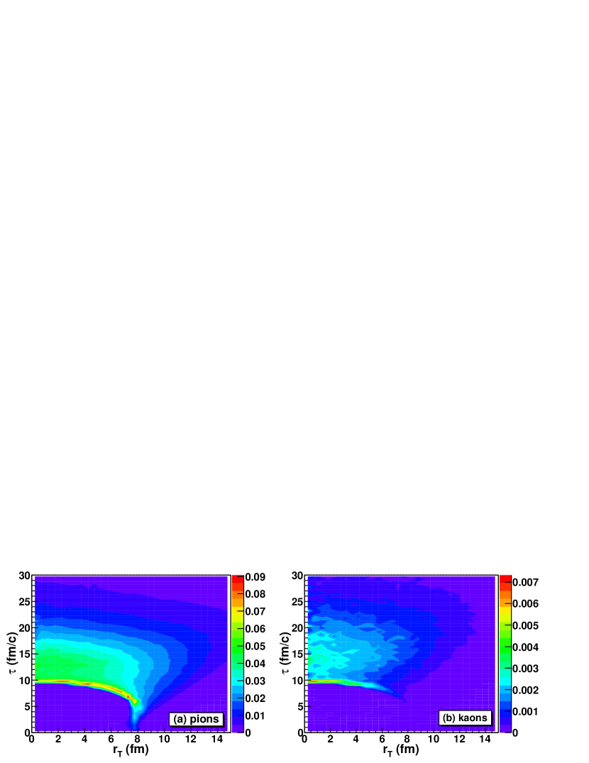
Figure 4: The momentum angle averaged emission functions per units of space-time and momentum rapidities $g(\tau,r_{T},p_{T})$ [fm^-3] (see body text) for pions (a) and kaons (b) obtained from the HKM simulations of Pb+Pb collisions at the LHC $\sqrt{s_{NN}}=2.76$ GeV, $0.2<p_{T}<0.3$ GeV/$c$, $|y|<0.5$, $c=0-5$%.

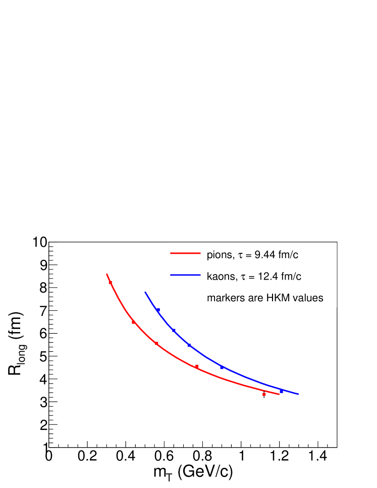
Figure 5: The same as in Fig. 1, 2 but radii are calculated in the full HKM model including re-scattering stage. To reduce the effect of the non-Gaussian correlation functions, we take more narrow fitting range for them, $q=0-0.04$ GeV/$c$. The fit parameters $T$ and $\alpha$ correspond to combined pion and kaon spectra fitting. At $T_{\pi}=147$ MeV, $T_{K}=141$ MeV, $\alpha_{\pi}=8.5$ and $\alpha_{K}=1.5$ extracted maximal emission times are $\tau_{\pi}=9.44\pm 0.02$ fm/$c$ and $\tau_{K}=12.40\pm 0.04$ fm/$c$.

Next, if we apply Eq. (8) to description of the femtoscopy radii obtained from the fits to pion and kaon HKM correlation functions in a broader range (e. g. $q=0-0.2$ GeV/$c$) Shap , covering not only their bell-like parts, but also the flatter ones, we will get unsatisfactory model data description for kaons using the fit parameters corresponding to spectra combined fit (see Fig. 6, blue solid line) with $T_{K}=141$ MeV, $\alpha_{K}=1.5$, and $\tau_{K}=11.09\pm 0.02$ fm/$c$. As for pions, they are described well with parameters restricted by combined spectra fit: $T_{\pi}=141$ MeV, $\alpha_{\pi}=1.82$, $\tau_{\pi}=10.34\pm 0.06$ fm/$c$. To get more or less adequate fit for the kaon longitudinal radius corresponding to wide $q$-region, one should remove constraints on $\alpha_{K}$ parameter. The dashed blue line in Fig. 6 represents such a fit with still constrained temperature, $T=144\pm 3$ MeV, and free $\alpha_{K}$ and $\tau_{K}$. The resulting fit at $T=146$ MeV and $\alpha=0.02$ provides good data description and gives $\tau_{K}=12.65\pm 1.58$ fm/$c$, that is in good agreement with the previous results for radii extracted at $q=0-0.04$ GeV/$c$ and the emission picture in Fig. 4. Therefore, the combined fit (with common temperature) for the pion and kaon spectra leads to the reliable estimate of the maximal particle emission times in the case of fitting only the peak of the non-Gaussian correlation function. The same good estimates can be extracted also from the Gaussian fit in large $q$-diapason, but for kaons $\alpha_{K}$ parameter has to be fitted without restrictions coming from common pion and kaon spectra fitting.

The difference as compared to the previous results for “without re-scattering” regime as well as an essential difference between the main fit parameters for pions and kaons mean that the re-scattering plays an important role in violation of $m_{T}$ scaling, in addition to transverse flow. The very small $\alpha$ value in kaon fit can indicate that the re-scattering stage affects seriously kaon emission picture and the re-scattering contribution to the femtoscopy scale cannot be described basing on the pure hydrodynamic (plus the resonance decays near freeze-out hypersurface) approach. The peculiarities of the re-scattering for kaons leads to more pronounced non-Gaussian character of the correlation function shape than for pions and also to a distortion of the femtoscopic scales $m_{T}$-dependence. It is found that for compensation of the influence of such a factor on the extracted effective time of maximal emission, in the case of wide $q$-fitting range for kaons, one can eliminate restriction for the parameter $\alpha$ coming from combined pion and kaon spectra fit.

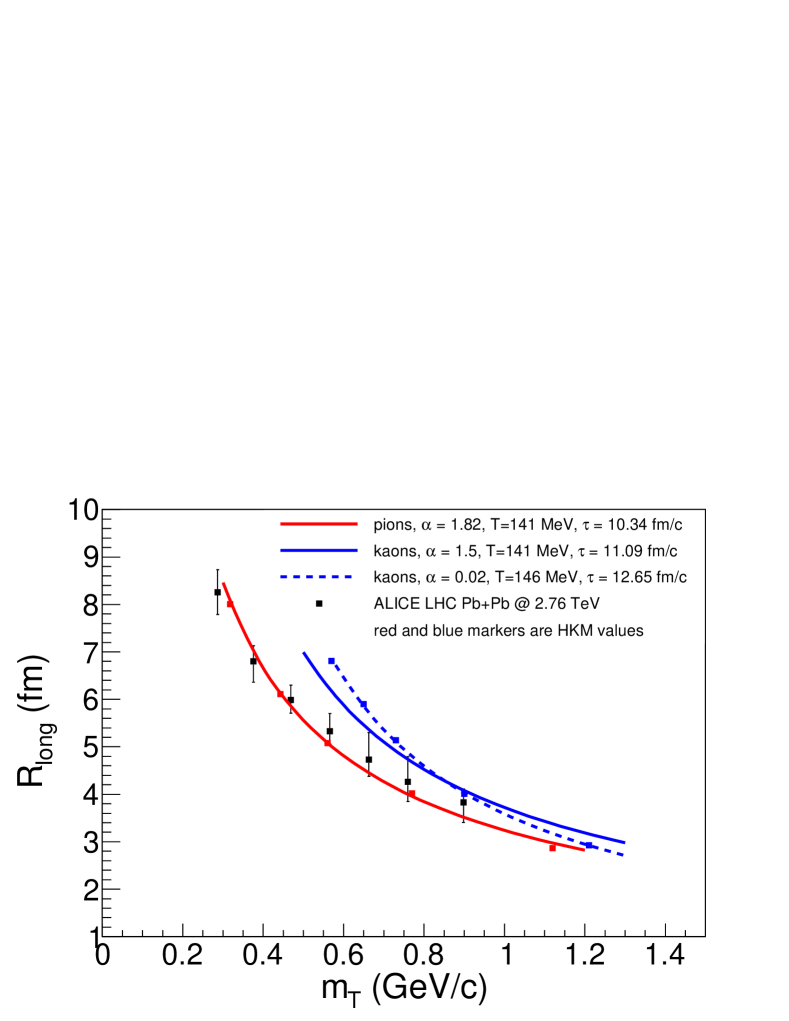
Figure 6: The same as in Fig. 5 but the radii are extracted from the fits to full HKM correlation functions in a wide $q$ range, $q=0-0.2$ GeV/$c$. Thus, the significant deviation of the CF shape from the Gaussian one leads to a distorted radii $m_{T}$-behavior. At fitting it can be compensated by decreasing $\alpha_{K}$ as compared to that obtained from the spectra fit. Experimental data AliceNew for pions are demonstrated for comparison.

In some sense a complementary method of obtaining the information about the space-time structure of the system from the correlation measurements, is known as the source imaging BrownDan1 ; Stab ; BrownDan2 aiming to extract the source function $S({\bf r}^{*})$, that represents the time-integrated distribution of particle emission points separation ${\bf r}^{*}$ in the pair rest frame. The analysis of the experimental data for baryon correlations, often based on the Lednicky-Lyuboshitz formula LL , supposes isotropic Gaussian separation distribution described by single width parameter $r_{0}$. This value can be extracted from the Gaussian fit to the angle-averaged source function $S(r)=1/(4\pi)\int_{0}^{2\pi}\int_{0}^{\pi}S(r,\theta,\phi)\sin\theta d\theta d\phi$. In this paper we also try to apply the fitting function (8) to pion, kaon, proton and proton-$\Lambda$ pairs to describe the $m_{T}$ dependence of source radii $r_{0}$ extracted from the corresponding angle-averaged source functions $S({\bf r}^{*})$ in HKM by means of Gaussian fits to them, see details in Ref. ShapSin . The results are presented in Fig. 7. At this fitting the temperature $T$ was constrained according to the combined pion and kaon spectra fit result $T=144\pm 3$ MeV, while $\alpha$ and $\tau$ were left free. The fits are unexpectedly good with the parameters $T=141$ MeV for all the particle pairs, $\tau_{\pi\pi}=11.47\pm 0.03$ fm/$c$, $\tau_{KK}=11.26\pm 0.04$ fm/$c$, $\tau_{pp}=11.30\pm 0.13$ fm/$c$, $\tau_{p\Lambda}=12.44\pm 0.29$ fm/$c$. The parameter $\alpha$ for all the pairs is about $10^{4}$ and more, i. e. actually $\alpha\rightarrow\infty$. The latter means that there are no transverse flows in the pair rest frame, saddle point in transverse velocity is zero for fluid elements in rest, that is natural. Found $m_{T}$-scaling (for proton-$\Lambda$ pairs $m_{T}=\sqrt{\left(\frac{m_{p}+m_{\Lambda}}{2}\right)^{2}+k_{T}^{2}}$) with slightly variative multiplier $\tau$ looks very surprising.

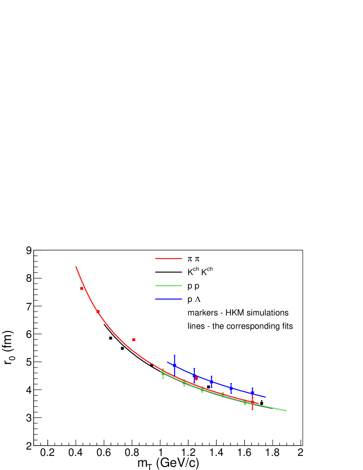
Figure 7: The $m_{T}$ dependencies of $\pi\pi$, $K^{ch}K^{ch}$, $pp$ and $p\Lambda$ source radii $r_{0}$ extracted from corresponding angle-averaged source functions calculated in HKM for $\sqrt{s_{NN}}=2.76$ GeV Pb+Pb collisions at the LHC, $c=0-5\%$, $|\eta|<0.8$. Transverse momentum ranges are $0.14<p_{T}<1.5$ GeV/$c$ for pions and kaons, $0.7<p_{T}<4.0$ GeV/$c$ for protons and $0.7<p_{T}<5.0$ GeV/$c$ for Lambdas.

Let us also apply the result (8) to $p+p$ collisions at LHC energy $\sqrt{s}=7$ TeV. The theoretical results for the pion interferometry radii in $p+p$ collisions with different particle multiplicity accounting for uncertainty principle in small systems were presented in Ref. PBM-Sin . The results without re-scattering are almost the same as in full HKM. Therefore we assume the temperature of chemical freeze-out to be 165 MeV. In Figs. 8, 9 we fit by f-la (8) these results obtained in the full HKM model, including re-scattering at the afterburner stage and corrections accounting for quantum uncertainty principle. One can see that, as it is expected, the values of $\tau$ in fitting function are much smaller than in Pb+Pb collisions, namely, in the multiplicity bin with mean charged particle multiplicity 17.9 we obtained $\tau=1.83\pm 0.02$ fm/$c$, $\alpha=13.9\pm 0.22$. At the same time for smaller mean multiplicity 9.2 both values are smaller: $\tau=1.60\pm 0.04$ fm/c, $\alpha=9.52\pm 0.44$.

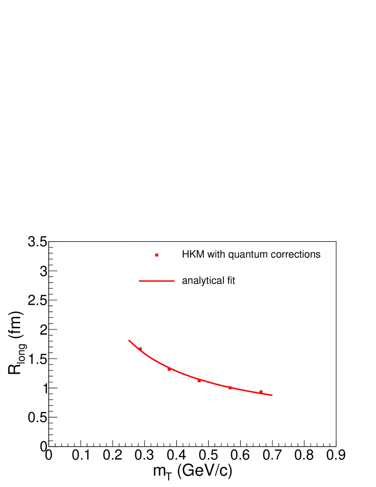
Figure 8: The $m_{T}$ dependence of pion longitudinal femtoscopy radius $R_{l}$ calculated in the full HKM model with corrections accounting for quantum uncertainty principle (red markers) together with the corresponding fit (8) (red line). The temperature is $T=165$ MeV, $\tau_{\mathrm{HKM}}=1.60\pm 0.04$ fm/$c$ and $\alpha=9.52\pm 0.44$. The results are related to $\sqrt{s}=7$ TeV $pp$ collisions at the LHC, $\langle dN_{ch}/d\eta\rangle=9.2$.

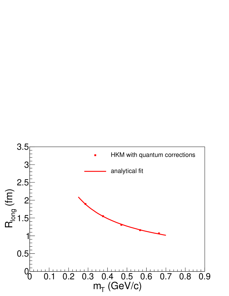
Figure 9: The same as in Fig. 8 for collision events with $\langle dN_{ch}/d\eta\rangle=17.9$. The values of the fit parameters are $\tau_{\mathrm{HKM}}=1.83\pm 0.02$ fm/$c$, $\alpha=13.9\pm 0.22$.

IV Conclusions

The analytical formula for the longitudinal interferometry radii that allows one to extract the time of maximal emission for the certain hadron pairs in the case of strong transverse flows in A+A and $p+p$ collision processes is proposed. It is compared with detail calculations and spatiotemporal picture of the particle emission in hydrokinetic model that already described well the large number of the bulk observables. Within such an analysis the factors were clarified affecting the interferometry radii and leading to violation of $m_{T}$-scaling between pions and kaons. They are: strong transverse flows, re-scattering and resonance decays at the afterburner stage and non-Gaussian form of the correlation function. It is found that for compensation of the influence of the latter factor on the extracted effective time of maximal emission for kaons, one may eliminate restriction on the “flow intensity” parameter $\alpha$ for kaons which follows from combined pion and kaon spectra fit.

As for the pion interferometry radii in $p+p$ collisions, the analytical fits to the corresponding HKM calculations give quite reasonable estimates for the times of the maximal emission for the collisions with different multiplicities.

The fitting formula has been applied also to the so-called source radii obtained from the Gaussian fit to the source function describing the dependence of the pair production on the distance between the two emitted particles in the rest frame of the pair. The pion-pion, kaon-kaon, proton-proton and proton-$\Lambda$ pairs produced in Pb+Pb collisions at the LHC were analyzed within HKM. Very surprisingly, it was found that analytical fit with slightly different $\tau$ for different pairs and with the other common adequate parameters — no transverse flow in the pair rest frame and the same temperature taken from combined pion and kaon spectra fit — gives very good result and leads to the $m_{T}$ scaling behavior of angle-averaged source radii for all mentioned baryon and meson pairs.

We hope that the results will be especially interesting for the experimentalists for simple fitting of the femtoscopy data and extracting the time of maximal emission in continuously emitting fireballs.

V Acknowledgment

The authors are grateful to L. V. Malinina for fruitful discussions and to Iu. A. Karpenko as one of the authors of HKM. The research was also carried out within the scope of the EUREA: European Ultra Relativistic Energies Agreement (European Research Group: “Heavy ions at ultrarelativistic energies”), and is further supported by the National Academy of Sciences of Ukraine (Agreements F5-2015 and MVC-2015).

References

- (1) S. Pratt, Phys. Rev. D 33 (1986) 1314.
-
(2)
A.N. Makhlin, Yu.M. Sinyukov, Sov. J. Nucl. Phys. 46 (1987) 345;
A. N. Makhlin, Yu. M. Sinyukov, Z. Phys. C 39 (1988) 69. - (3) Yu. M. Sinyukov, Nucl. Phys. A 498 (1989) 151.
- (4) Y. Hama, S.S. Padula, Phys. Rev. D 37 (1988) 3237.
- (5) G.I. Kopylov, M.I. Podgoretsky, Sov. J. Nucl. Phys. 15 (1972) 219; 15 (1972) 219 18 (1973) 336; 19 (1974) 215.
- (6) S. E. Koonin, Phys. Lett. B 70, 43 (1977).
- (7) V. M. Shapoval, P. Braun-Munzinger, Iu. A. Karpenko, Yu. M. Sinyukov, Nucl. Phys. A 929 (2014) 1.
- (8) Yu.M. Sinyukov, S.V. Akkelin, and Y. Hama, Phys. Rev. Lett. 89 (2002) 052301.
- (9) S.V. Akkelin, Y. Hama, Iu.A. Karpenko, Yu.M. Sinyukov, Phys. Rev. C 78 (2008) 034906.
- (10) Iu.A. Karpenko, Yu.M. Sinyukov, Phys. Rev. C 81 (2010) 054903.
-
(11)
Iu.A. Karpenko, Yu.M. Sinyukov, K. Werner, Phys. Rev. C 87 (2013) 024914,
arXiv:1204.5351v2 [nucl-th]. - (12) Iu.A. Karpenko, Yu.M. Sinyukov, Phys. Lett. B 688 (2010) 50.
- (13) V. M. Shapoval, Yu. M. Sinyukov, Iu. A. Karpenko, Phys. Rev. C 88 (2013) 064904.
- (14) V. M. Shapoval, P. Braun-Munzinger, Iu. A. Karpenko, Yu. M. Sinyukov, Phys. Lett. B 725 (2013) 139.
- (15) W. Broniowski, M. Rybczynsky, P. Bozek, Comput. Phys. Commun. 180 (2009) 69; arXiv:0710.5731v3.
- (16) Yu.M. Sinyukov, S.V. Akkelin, Y. Hama, Iu.A. Karpenko, Act. Phys. Pol. B 40 (2009) 1025.
- (17) F. Cooper and G. Frye, Phys. Rev. D 10, 186 (1974).
- (18) S.V. Akkelin, Yu.M. Sinyukov, Phys. Lett. B 356 (1995) 525.
- (19) S.V. Akkelin, Yu.M. Sinyukov, Z. Phys. C 72 (1996) 501.
- (20) Yu.M. Sinyukov, S.V. Akkelin, A.Yu. Tolstykh, Nucl. Phys. A 72 (1996) 278c.
- (21) M. Herrmann, G.F. Bertsch, Phys. Rev. C 51 (1995) 328.
- (22) B. Abelev et al. (ALICE Collaboration), Phys. Rev. C 88 (2013) 044910.
- (23) J. Adam, et al. (ALICE Collaboration), arXiv:1507.06842 [nucl-ex].
- (24) D.A. Brown and P. Danielewicz, Phys. Lett. B 398, 252 (1997).
- (25) D.A. Brown and P. Danielewicz, Phys. Rev. C 57, 2474 (1998).
- (26) D.A. Brown and P. Danielewicz, Phys. Rev. C 64, 014902 (2001).
- (27) R. Lednický, V. L. Lyuboshitz, Yad. Fiz. 35, 1316 (1981) [Sov. J. Nucl. Phys. 35, 770 (1982)]; in Proceedings of the International Workshop on Particle Correlations and Interferometry in Nuclear Collisions (CORINNE 90), Nantes, France, 1990, edited by D. Ardouin (World Scientific, Singapore, 1990), pp. 42–54; R. Lednicky, J. Phys. G: Nucl. Part. Phys. 35 (2008) 125109.
- (28) K. Aamodt, et al. (ALICE Collaboration), Phys. Rev. D 84 (2011) 112004.