Abstract

We perform a comprehensive study of charged lepton flavour violation in Randall-Sundrum (RS) models in a fully 5D quantum-field-theoretical framework. We consider the RS model with minimal field content and a “custodially protected” extension as well as three implementations of the IR-brane localized Higgs field, including the non-decoupling effect of the KK excitations of a narrow bulk Higgs. Our calculation provides the first complete result for the flavour-violating electromagnetic dipole operator in Randall-Sundrum models. It contains three contributions with different dependence on the magnitude of the anarchic 5D Yukawa matrix, which can all be important in certain parameter regions. We study the typical range for the branching fractions of $\mu\to e\gamma$, $\mu\to 3e$, $\mu N\to eN$ as well as $\tau\to\mu\gamma$, $\tau\to 3\mu$ and the electron electric dipole moment by a numerical scan in both the minimal and the custodial RS model. The combination of $\mu\to e\gamma$ and $\mu N\to eN$ currently provides the most stringent constraint on the parameter space of the model. A typical lower limit on the KK scale $T$ is around $2\,{\rm TeV}$ in the minimal model (up to 4 TeV in the bulk Higgs case with large Yukawa couplings), and around $4\,{\rm TeV}$ in the custodially protected model, which corresponds to a mass of about 10 TeV for the first KK excitations, far beyond the lower limit from the non-observation of direct production at the LHC.

TUM-HEP-1007/15
OUTP-15-13P
arXiv:1508.01705 [hep-ph]
August 05, 2015

Lepton flavour violation in RS models with a brane- or nearly brane-localized Higgs

M. Beneke^a, P. Moch^a and J. Rohrwild^b
aPhysik Department T31, James Franck-Straße 1
Technische Universität München,
D–85748 Garching, Germany
^bRudolf Peierls Centre for Theoretical Physics,
University of Oxford, 1 Keble Road,
Oxford OX1 3NP, United Kingdom

1 Introduction

Rare lepton decays are among the promising indirect probes for physics beyond the Standard Model (SM). This is especially true for processes featuring lepton-flavour violation (LFV). For such decays the SM contribution vanishes for all practical purposes due to the small neutrino masses, and the experimental signature is typically very clean. The absence of a SM background makes the study of the decays $\mu\to e\gamma$ and $\mu\to 3e$ as well as muon-to-electron conversion in nuclei in extensions of the SM also theoretically cleaner than the study of lepton observables unrelated to flavour violation. The reason for this is that in the latter case the search for new physics involves the search for tiny deviations in observables such as $(g-2)_{\mu}$, which must then be measured and predicted to very high precision.

The warped extra-dimensional Randall-Sundrum (RS) models, originally introduced to address the relative weakness of gravity [1] and the gauge-gravity hierarchy problem [2], generically also have a rich flavour structure. Further, they provide a geometric interpretation for the flavour hierarchies observed in the SM: the wave functions of SM fermions in the fifth dimension when localized to varying degree naturally generate a hierarchical flavour sector [3, 4, 5, 6]. Despite the fact that the RS model is to some extent protected from large flavour-changing neutral currents (FCNCs) [7], the strongest constraint on the scale of the extra dimension comes from Kaluza-Klein (KK) gluon mediated $\Delta F=2$ processes—notably in the kaon system [8]. However, these bounds can, to some degree, be avoided by imposing some structure on the quark Yukawa matrices in the five-dimensional (5D) theory [9] or by extending the strong gauge group [10]. Nonetheless, direct searches at the LHC for KK states are no longer very promising as the scales that can be probed in direct production are comparably low. This is precisely the situation were low-energy precision observables can help considerably constraining the model.

In this work we calculate the lepton-flavour violating four-fermion and electromagnetic dipole operators induced by the RS bulk fields at the tree- and one-loop level, respectively. We then study the $\mu\to 3e$ and $\mu\to e\gamma$ transitions, and muon-to-electron conversion in nuclei in the minimal and custodially protected RS model with three different implementations of the Higgs field localized on or near the TeV brane of the model. Lepton-flavour violating processes have been studied in the context of the RS model in the past, beginning with [6, 11, 12]. Particularly relevant are [13], which gives the first comprehensive analysis of charged LFV, and [14] with the first fully five-dimensional treatment of loop effects, which dominate the $\mu\to e\gamma$ decay. However, neither of the two can be said to provide a complete description of the loop-induced dipole operator coefficient, which leads us to reconsider LFV phenomenology building on our recent work [15, 16, 17] on penguin transitions in the RS model. In this approach we integrate out the five-dimensional (5D) bulk and match the RS model on the SM extended by gauge-invariant dimension-six operators [18, 19], which is then used to study the processes of interest. This two-step procedure is justified, since the scale of the fifth dimension, related to the mass of the lightest KK excitation, is already constrained to be much larger than the electroweak scale. This approach allows for a transparent and complete calculation of gauge- and Higgs-boson exchange induced dipole transitions, which has already been applied to the flavour-diagonal case of the anomalous magnetic moment of the muon [15, 16, 17]. Here we focus on the flavour-changing leptonic transitions. We also add a 5D treatment of the bulk Higgs and the non-decoupling effect in the localization limit recently pointed out in [20]. Depending on the exact realization of the RS model loop-effects can be sizeable also for $\mu\to 3e$ and muon conversion, which at first glance are dominated by tree-level physics, and may introduce new correlations between $\mu\to e\gamma$ and those observables. In our study we do not impose additional flavour symmetries on the Yukawa matrices of the model and stick to the so-called minimal and custodially protected models. This implies that we do not attempt here a description of neutrino masses and mixing in the RS framework – in the minimal RS model the neutrinos remain massless – and only consider charged lepton flavour violation, which arises in the RS models independent from neutrino masses. In order to simultaneously generate hierarchical charged lepton masses and large neutrino mixing, RS models with additional flavour structure such as minimal flavour violation or discrete symmetries were considered [21, 22, 23], as well as mechanisms to suppress lepton flavour violation [24, 25]. These have implications for LFV at tree-level, even eliminating tree-level LFV completely, but do not modify the structure of loop-induced LFV processes, whose complete computation is the main result of this work.

The outline of this paper is as follows. The starting point of our analysis in Section 2 is the effective SM Lagrangian including dimension-six operators. We restrict ourselves to operators that can be generated in the Randall-Sundrum model at tree-level and to loop-induced dipole operators relevant to LFV processes. After expressing the Lagrangian in terms of fields in the broken phase, we match onto an effective low-energy theory. This allows us to use results from the literature to determine the LFV observables as functions of the dimension-six operator short-distance coefficients. In Section 3 we discuss three variants of localizing the Higgs field on or near the TeV brane and give the results for the corresponding short-distance coefficients in the minimal and custodially protected RS models using and extending results from [15, 17]. LFV phenomenology of $\mu\to e\gamma$, $\mu\to 3e$ and $\mu-e$ conversion and the correlations among these observables are presented in Section 4. We further correlate these observables with the electron electric dipole moment (EDM) and compare the constraining power of present limits on LFV observables and the electron EDM. We conclude in Section 5.

2 From the 5D theory to low-energy observables

In conformal coordinates the metric for the five-dimensional space-time of the Randall-Sundrum model is given by

$$ds^{2}=\left(\frac{1}{kz}\right)^{\!2}\left(\eta_{\mu\nu}dx^{\mu}dx^{\nu}-dz^{2}\right),$$ (1)

where $k=2.44\cdot 10^{18}\,$GeV is of order of the Planck scale $M_{\rm Pl}$. The fifth coordinate $z$ can take values from $z=1/k$ (Planck brane) to $z=1/T$ (IR brane). The scale $T$ determines the mass of the KK excitations in the effective 4D spectrum and is assumed to be of the order of a few TeV. We denote by $\epsilon=T/k$ the small ratio of the two scales.

The specific RS model is characterised by the particle content and the associated boundary conditions on the two branes. The two most common models are the minimal and the custodially protected model [28, 29]. The latter has an extended particle spectrum and gauge group to enforce a protection mechanism for the electroweak $\rho$ parameter and the $Zb\bar{b}$ vertex. In both models the Higgs is localized on or close to the IR brane. The prescription how the Higgs is localized is part of the model setup itself, see also [30, 31]. Here we will closely follow the notation and conventions of [15, 17] for the minimal RS model and the model with custodial protection. We therefore refer to these references for the exact definition of the 5D Lagrangians.

However, it is useful to introduce the parameters of the 5D Lagrangian relevant for the study of lepton-flavour violation. The 5D Lagrangian contains two parameter sets related to flavour. On the one hand there is the 5D mass $M_{\psi_{i}}$ for each 5D fermion field $\psi_{i}$. The corresponding dimensionless 5D mass parameter is $c_{\psi_{i}}=M_{\psi_{i}}/k$. To obtain a phenomenologically viable low-energy theory that reproduces the measured lepton masses the $c_{\psi_{i}}$ have to take values not too far from $1/2$ for SU(2) doublets and from $-1/2$ for singlets. On the other hand, the 5D Higgs Lagrangian incorporates 5D Yukawa couplings $y^{\rm(5D)}$. It is customary to work with the dimensionless Yukawa matrices $Y=y^{\rm(5D)}\,k$ in the minimal model, and $Y,Y_{u}$ in the custodial model. We generally assume that each is roughly $\mathcal{O}(1)$ and anarchic. Furthermore, the Higgs field is localized on or near the IR brane. There are several ways to do this. A genuine brane Higgs is exactly localized on the IR brane and its potential 5D structure cannot be resolved by construction. An IR localized bulk Higgs can be resolved, and one also needs to consider possible effects of Kaluza-Klein states of the Higgs as was pointed out in [20]. If the Higgs is exactly brane-localized one can in principle introduce a separate Yukawa coupling for the coupling of right-handed doublets and left-handed singlet to the Higgs. However, for simplicity we assume that these so-called wrong-chirality Higgs couplings [13, 32] are equal to their “normal” counterparts. In the following, we only discuss the different Higgs localizations separately if they give rise to distinct results.

Ultimately, we match the full 5D Lagrangian onto an effective 4D dimension-six Lagrangian following [15] and determine the physically interesting observables as functions of the corresponding Wilson coefficients. The matching calculation is performed in Sec. 3. In the remainder of this section we take the SM effective theory including dimension-six operators as the starting point to compute the low-energy observables. We will consider only operators of dimension six that can be generated by the RS model at tree- or one-loop level.

2.1 The dimension-six Lagrangian

Let us start by considering the effective SU(2)$\times$U(1)-symmetric Lagrangian up to dimension six,

$$\mathcal{L}=\mathcal{L}_{\rm SM}+\frac{1}{T^{2}}\,\mathcal{L}^{\rm dim-6}+\text{higher-dimensional operators}\,,$$ (2)

where we did not include the single dimension-five operator as it cannot contribute to charged LFV. We also extracted the scale, where the effective description breaks down, given by $T$ in the RS model. At dimension six the operators relevant to the following analysis of LFV observables can be taken directly from [19, 18]

$$\mathcal{L}^{\rm dim6}_{\rm LFV} = a^{B}_{ij}(\bar{L}_{i}\sigma^{\mu\nu}E_{j})\Phi B_{\mu\nu}+a^{W}_{ij}(\bar{L}_{i}\tau^{A}\sigma^{\mu\nu}E_{j})\Phi W^{A}_{\mu\nu}+{\rm h.c.}$$ (3)

$$+\,b^{LL}_{ijkl}(\bar{L}_{i}\gamma^{\mu}L_{j})(\bar{L}_{k}\gamma_{\mu}L_{l})+b^{LE}_{ij}(\bar{L}_{i}\gamma^{\mu}L_{i})(\bar{E}_{j}\gamma_{\mu}E_{j})+b^{EE}_{ij}(\bar{E}_{i}\gamma^{\mu}E_{i})(\bar{E}_{j}\gamma_{\mu}E_{j})$$

$$+\,c^{1}_{ij}\Phi^{\dagger}i\overleftrightarrow{D}^{\!\mu}\Phi(\bar{E}_{i}\gamma_{\mu}E_{j})+c^{2}_{ij}\Phi^{\dagger}i\overleftrightarrow{D}^{\!\mu}\Phi(\bar{L}_{i}\gamma_{\mu}L_{j})+c^{3}_{ij}\Phi^{\dagger}i\overleftrightarrow{\tau^{A}D}^{\mu}\Phi(\bar{L}_{i}\tau^{A}\gamma_{\mu}L_{j})$$

$$+\,h_{ij}(\Phi^{\dagger}\Phi)\bar{L}_{i}\Phi E_{j}+\mbox{ h.c.}$$

$$+\,\sum_{\ell=E,L}\,\sum_{q=Q,U,D}b^{\ell q}_{ij}(\bar{\ell}_{i}\gamma^{\mu}\ell_{i})(\bar{q}_{j}\gamma_{\mu}q_{j})+b^{L\tau Q}_{ij}(\bar{L}_{i}\tau^{A}\gamma^{\mu}L_{i})(\bar{Q}_{j}\tau^{A}\gamma_{\mu}Q_{j})\,,$$

where $L$ ($Q$) denotes doublet and $E$ ($U,D$) singlet lepton (quark) fields. Furthermore, $\Phi^{\dagger}\overleftrightarrow{i\tau^{A}D}_{\mu}\Phi=\frac{1}{2}(\Phi^{\dagger}i\tau^{A}D_{\mu}\Phi-\Phi^{\dagger}i\overleftarrow{D}_{\mu}\tau^{A}\Phi)$ and $\Phi^{\dagger}\overleftrightarrow{D}_{\mu}\Phi=\frac{1}{2}(\Phi^{\dagger}D_{\mu}\Phi-({D}_{\mu}\Phi)^{\dagger}\Phi)$ with the covariant derivative defined as

$$D_{\mu}=\partial_{\mu}-ig^{\prime}\frac{Y}{2}B_{\mu}-ig{T^{A}}{W^{A}_{\mu}}\,,$$ (4)

and $T^{A}$ the SU(2) generators in the appropriate representation (e.g. $T^{A}=\tau^{A}/2$ with $\tau^{A}$ the Pauli matrices for the doublet), and $Y$ the hypercharge. The hermitian conjugate in (3) only applies to terms in the same line. Of all the operators given in (3) only the dipole operators in the first line cannot be generated at tree-level in the RS model. The restricted flavour structure of some of the four-fermion operators anticipates properties of the RS model at the tree-level. Even though we aim to study lepton flavour violation, the operators with two quark and two lepton fields have to be included in $\mathcal{L}^{\rm dim6}_{LFV}$, since they contribute to muon conversion in nuclei.

The transition from the theory with unbroken to the one with broken electroweak gauge symmetry proceeds via the standard substitution rules,

$$\Phi\to\begin{pmatrix}\phi^{+}\\ \frac{1}{\sqrt{2}}(v+h+iG)\end{pmatrix} L_{i}\to U_{ij}P_{L}\begin{pmatrix}\nu_{j}\\[5.69046pt] \ell_{j}\end{pmatrix} E_{i}\to V_{ij}P_{R}\ell_{j}$$ (5)

$$Q_{i}\to P_{L}\begin{pmatrix}U^{u}_{ij}u_{j}\\ U^{d}_{ij}d_{j}\end{pmatrix} U_{i}\to V^{u}_{ij}P_{R}u_{j} D_{i}\to V^{d}_{ij}P_{R}d_{j}$$ (6)

and

$$D_{\mu}\to\partial_{\mu}-ieQA_{\mu}-\frac{ig}{c_{W}}(T^{3}-s^{2}_{W}Q)Z_{\mu}-\frac{ig}{\sqrt{2}}(T^{1}+iT^{2})W^{+}_{\mu}-\frac{ig}{\sqrt{2}}(T^{1}-iT^{2})W^{-}_{\mu},$$ (7)

with $Z_{\mu}=c_{W}W^{3}_{\mu}-s_{W}B_{\mu}$, and $A_{\mu}=c_{W}B_{\mu}+s_{W}W^{3}_{\mu}$. Inserting (5) and (7) into (3) generates many operators, most of which cannot contribute to the processes we are interested in, see [15] for details. We are only concerned with operators that can contribute at tree-level (if they are generated at loop- or tree-level in the full 5D theory) or at loop-level (if they are generated already at tree-level). This leaves us with the Lagrangian

$$\mathcal{L}^{\rm dim6}_{LFV}\to\mathcal{L}^{\rm broken}_{LFV}= \;\frac{\alpha^{A}_{ij}+{\alpha^{A}_{ji}}^{\star}}{2}\frac{v}{\sqrt{2}}\,(\bar{\ell}_{i}\sigma^{\mu\nu}\ell_{j})F_{\mu\nu}+\;\frac{\alpha^{A}_{ij}-{\alpha^{A}_{ji}}^{\star}}{2}\frac{v}{\sqrt{2}}\,(\bar{\ell}_{i}\sigma^{\mu\nu}\gamma_{5}\ell_{j})F_{\mu\nu}$$

$$+\beta^{EE}_{ijkl}(\bar{\ell}_{i}\gamma^{\mu}P_{R}\ell_{j})(\bar{\ell}_{k}\gamma_{\mu}P_{R}\ell_{l})+\beta^{LE}_{ijkl}(\bar{\ell}_{i}\gamma^{\mu}P_{L}\ell_{j})(\bar{\ell}_{k}\gamma_{\mu}P_{R}\ell_{l})$$

$$+\beta^{LL}_{ijkl}(\bar{\ell}_{i}\gamma^{\mu}P_{L}\ell_{j})(\bar{\ell}_{k}\gamma_{\mu}P_{L}\ell_{l})$$

$$-{\gamma}^{1}_{ij}\frac{gv^{2}}{4c_{W}}Z^{\mu}(\bar{\ell}_{i}\gamma_{\mu}P_{R}\ell_{j})-[{\gamma}^{2}_{ij}+\gamma^{3}_{ij}]\frac{gv^{2}}{4c_{W}}Z^{\mu}(\bar{\ell}_{i}\gamma_{\mu}P_{L}\ell_{j})$$

$$+{\gamma}^{3}_{ij}\frac{gv^{2}}{2\sqrt{2}}W^{+,\mu}(\bar{\nu}_{i}\gamma_{\mu}P_{L}\ell_{j})+{\text{h.c.}}$$

$$+\eta_{ij}\frac{3v^{2}}{2}\frac{h}{\sqrt{2}}(\bar{\ell}_{i}P_{R}\ell_{j})+\eta_{ij}\frac{v^{3}}{2\sqrt{2}}(\bar{\ell}_{i}P_{R}\ell_{j})+{\text{h.c.}}$$

$$+\beta^{Eu}_{ijkl}(\bar{\ell}_{i}\gamma^{\mu}P_{R}\ell_{j})(\bar{u}_{k}\gamma_{\mu}P_{R}u_{l})+\beta^{Ed}_{ijkl}(\bar{\ell}_{i}\gamma^{\mu}P_{R}\ell_{j})(\bar{d}_{k}\gamma_{\mu}P_{R}d_{l})$$

$$+\beta^{EQ}_{ijkl}(\bar{\ell}_{i}\gamma^{\mu}P_{R}\ell_{j})(\bar{u}_{k}\gamma_{\mu}P_{L}u_{l})+\beta^{EQ}_{ijkl}(\bar{\ell}_{i}\gamma^{\mu}P_{R}\ell_{j})(\bar{d}_{k}\gamma_{\mu}P_{L}d_{l})$$

$$+\beta^{Lu}_{ijkl}(\bar{\ell}_{i}\gamma^{\mu}P_{L}\ell_{j})(\bar{u}_{k}\gamma_{\mu}P_{R}u_{l})+\beta^{Ld}_{ijkl}(\bar{\ell}_{i}\gamma^{\mu}P_{L}\ell_{j})(\bar{d}_{k}\gamma_{\mu}P_{R}d_{l})$$

$$+(\beta^{LQ}_{ijkl}-\beta_{ijkl}^{L\tau Q})(\bar{\ell}_{i}\gamma^{\mu}P_{L}\ell_{j})(\bar{u}_{k}\gamma_{\mu}P_{L}u_{l})$$

$$+(\beta^{LQ}_{ijkl}+\beta_{ijkl}^{L\tau Q})(\bar{\ell}_{i}\gamma^{\mu}P_{L}\ell_{j})(\bar{d}_{k}\gamma_{\mu}P_{L}d_{l})\,,$$ (8)

with $P_{L/R}=\frac{1}{2}(1\mp\gamma_{5})$, and

$$\alpha^{A}_{ij} =[U^{\dagger}a^{A}V]_{ij}\,, \gamma^{1}_{ij} =\sum_{m,n}\,[V^{\dagger}]_{im}V_{nj}\,c^{1}_{mn}\,,$$

$$\eta_{ij} =\sum_{n,m}[U^{\dagger}]_{im}h_{mn}V_{nj}\,, \gamma^{x}_{ij} =\sum_{m,n}\,[U^{\dagger}]_{im}U_{nj}\,c^{x}_{mn}\quad(x=2,3)\,,$$

$$\beta^{LL}_{ijkl} =\sum_{m,n,o,p}\,[U^{\dagger}]_{im}U_{nj}[U^{\dagger}]_{ko}U_{pl}\,b^{LL}_{mnop}\,, \beta^{FF^{\prime}}_{ijkl} =\sum_{m,n}\,[M^{\dagger}]_{im}M_{mj}[M^{\prime\dagger}]_{kn}M^{\prime}_{nl}\,b^{FF^{\prime}}_{mn}\,.$$ (9)

Here $a^{A}_{ij}=c_{W}a^{B}_{ij}-s_{W}a^{W}_{ij}$, $M^{(\prime)}\in\{U,V,U^{u},V^{u},U^{d},V^{d}\}$ are the appropriate flavour rotation matrices for the fermion $F^{(\prime)}$, and a similar definition applies to $\beta_{ijkl}^{L\tau Q}$.

2.2 From the effective Lagrangian to LFV observables

The main observables for charged lepton flavour violation are radiative transitions of the type $\ell_{1}\to\ell_{2}\gamma$, lepton conversion in a nucleus, and tri-lepton decays $\ell_{1}\to\ell_{2}\ell\ell$. These processes are usually studied in high intensity, low energy set-ups. The typical energy release of the process is the mass of the initial (charged) lepton, a muon or a tau. Starting from the effective Lagrangian at the electroweak scale discussed in the previous section, we construct an effective low-energy Lagrangian by integrating out the heavy gauge bosons and quarks and the fluctuations associated with scales above the charged lepton mass. For $\mu\to e\gamma$, muon conversion and $\mu\to 3e$ this low-energy theory has been discussed in great detail in the literature, see e.g. [27, 35], and especially [26].

We follow [26] and consider first the radiative decay $\mu\to e\gamma$. The Lagrangian takes the form

$$\mathcal{L}_{\mu\to e\gamma}= A_{R}m_{\mu}\bar{\ell}_{e}\sigma^{\sigma\rho}F_{\sigma\rho}P_{R}\ell_{\mu}+A_{L}m_{\mu}\bar{\ell}_{e}\sigma^{\sigma\rho}F_{\sigma\rho}P_{L}\ell_{\mu}+\mbox{h.c.}\,,$$ (10)

where the label on the field $\ell$ denotes the lepton flavour. This Lagrangian is supposed to be valid at scales below the electron mass—all quantum fluctuations involving leptons have been integrated out and have been absorbed into the two coefficients of the dipole operators. In fact instead of this Lagrangian we might just as well consider the general U(1)_em invariant vertex function for on-shell fermions (the photon momentum $q$ is ingoing)

$$\Gamma^{\mu}(p,p^{\prime}) = ieQ_{\ell}\bar{u}_{\mu}(p^{\prime},s^{\prime})\bigg{[}\gamma^{\mu}F_{1}(q^{2})+\frac{i\sigma^{\mu\nu}q_{\nu}}{2m_{\mu}}F_{2}(q^{2})+\frac{\sigma^{\mu\nu}q_{\nu}}{2m_{\mu}}\gamma_{5}F_{3}(q^{2})$$ (11)

$$+\,\left(q^{2}\gamma^{\mu}-\not{q}q^{\mu}\right)\gamma_{5}F_{4}(q^{2})\bigg{]}u_{e}(p,s)\,.$$

The on-shell dipole form factors of the electromagnetic muon-electron vertex are related to the coefficients $A_{L}$ and $A_{R}$ by

$$A_{R}=\frac{Q_{\ell}e(F_{2}(0)-iF_{3}(0))}{4m_{\mu}^{2}} A_{L}=\frac{Q_{\ell}e(F_{2}(0)+iF_{3}(0))}{4m_{\mu}^{2}}\,,$$ (12)

where $Q_{\ell}=-1$ is the electron charge in units of the positron charge $e$. Up to terms suppressed by powers of the electron mass the branching fraction can be written as

$${\rm{Br}}(\mu\to e\gamma)=\frac{m_{\mu}^{5}}{4\pi\Gamma_{\mu}}(|A_{L}|^{2}+|A_{R}|^{2})\,.$$ (13)

Here $\Gamma_{\mu}$ is the total decay width of the muon. The generalization to $\ell_{i}\to\ell_{j}\gamma$ is obvious.

The process $\mu\to 3e$ is described by the extended Lagrangian [26]

$$\mathcal{L}_{\mu\to 3e} = \,A_{R}m_{\mu}\bar{\ell}_{e}\sigma^{\sigma\rho}F_{\sigma\rho}P_{R}\ell_{\mu}+A_{L}m_{\mu}\bar{\ell}_{e}\sigma^{\sigma\rho}F_{\sigma\rho}P_{L}\ell_{\mu}$$ (14)

$$+\,g_{1}\,\bar{\ell}_{e}P_{R}\ell_{\mu}\;\bar{\ell}_{e}P_{R}\ell_{e}+g_{2}\,\bar{\ell}_{e}P_{L}\ell_{\mu}\;\bar{\ell}_{e}P_{L}\ell_{e}$$

$$+\,g_{3}\,\bar{\ell}_{e}\gamma^{\nu}P_{R}\ell_{\mu}\;\bar{\ell}_{e}\gamma_{\nu}P_{R}\ell_{e}+g_{4}\,\bar{\ell}_{e}\gamma^{\nu}P_{L}\ell_{\mu}\;\bar{\ell}_{e}\gamma_{\nu}P_{L}\ell_{e}$$

$$+\,g_{5}\,\bar{\ell}_{e}\gamma^{\nu}P_{R}\ell_{\mu}\;\bar{\ell}_{e}\gamma_{\nu}P_{L}\ell_{e}+g_{6}\,\bar{\ell}_{e}\gamma^{\nu}P_{L}\ell_{\mu}\;\bar{\ell}_{e}\gamma_{\nu}P_{R}\ell_{e}+\,\text{h.c.}\,.$$

Note that the coefficients $A_{L,R}$ and $g_{i}$ have mass dimension $-2$. The appearance of the same coefficients $A_{L,R}$ as in (10) indicates that all quantum fluctuations are again integrated out. In practice, absorbing e.g. electron loop diagrams involving a four-fermion operator into $A_{L,R}$ and into a loop correction to the $g_{i}$ is convenient as we do not have to treat the different lepton flavours separately. In particular, in writing (14) the effect of the off-shell ($q^{2}\neq 0$) form factors in (11) is absorbed into the $g_{i}$ coefficients (see the [26] for details). In any case, since this represents a loop correction to the Wilson coefficients which are already generated at the tree-level, we neglect these effects in our calculation.

The branching fraction of $\mu\to 3e$ can easily be expressed through the coefficients $g_{i}$ and $A_{L,R}$ [26]:

$${\rm Br}(\mu\to 3e) = \frac{m_{\mu}^{5}}{1536\pi^{3}\Gamma_{\mu}}\bigg{[}\frac{|g_{1}|^{2}+|g_{2}|^{2}}{8}+2(|g_{3}|^{2}+|g_{4}|^{2})+|g_{5}|^{2}+|g_{6}|^{2}$$ (15)

$$-\,8e\,{\rm{Re}}\left[A_{R}(2g_{4}^{*}+g_{6}^{*})+A_{L}(2g_{3}^{*}+g_{5}^{*})\right]$$

$$+\,64e^{2}(\ln\frac{m_{\mu}}{m_{e}}-\frac{11}{8})(|A_{L}|^{2}+|A_{R}|^{2})\bigg{]}$$

with $\Gamma_{\mu}$ the muon decay width. The first line arises from tree-level KK exchange in the RS model, while the second and third involve the loop-induced dipole operator coefficients. The reason for keeping these formally suppressed terms is not only the logarithmic enhancement paired with a large numerical coefficient. One-loop corrections to the $g_{i}$ may have a similar logarithmic enhancement and the large factors of 8 and 64 might be misleading, since it can be absorbed into the definition of the coefficients $A_{L,R}$, which come with a $1/(4\pi)^{2}$ loop suppression. The important point is that one-loop corrections to the $g_{i}$ introduce only a small shifts in the coefficients without altering the general properties. On the other hand, the dependence on $A_{L,R}$ implies sensitivity to different aspects of the underlying model. In RS models $A_{L,R}$ have a specific dependence on the Yukawa couplings, which can provide an important contribution to the branching fraction in sizeable parts of the model parameter space. In these regions the effect of $A_{L,R}$ should not be neglected, as it will significantly alter the signatures of the RS model in flavour observables.

Muon conversion in nuclei is mediated by both, operators containing quark fields and electromagnetic dipole operators. The effective Lagrangian is [26, 36]

$$\mathcal{L}_{\mu N\to eN} = A_{R}m_{\mu}\bar{\ell}_{e}\sigma^{\sigma\rho}F_{\sigma\rho}P_{R}\ell_{\mu}+A_{L}m_{\mu}\bar{\ell}_{e}\sigma^{\sigma\rho}F_{\sigma\rho}P_{L}\ell_{\mu}$$ (16)

$$+\,\sum_{q=u,d}c^{q}_{VR}\bar{\ell}_{e}\gamma^{\nu}P_{R}\ell_{\mu}\bar{q}\gamma_{\nu}q+\sum_{q=u,d}c^{q}_{VL}\bar{\ell}_{e}\gamma^{\nu}P_{L}\ell_{\mu}\bar{q}\gamma_{\nu}q$$

$$+\,\sum_{q=u,d,s}\frac{m_{q}m_{\mu}}{M_{H}^{2}}c^{q}_{SL}\bar{\ell}_{e}P_{R}\ell_{\mu}\bar{q}q+\sum_{q=u,d,s}\frac{m_{q}m_{\mu}}{M_{H}^{2}}c^{q}_{SR}\bar{\ell}_{e}P_{L}\ell_{\mu}\bar{q}q$$

$$+\,\frac{\alpha_{s}m_{\mu}}{M_{H}^{2}}c^{L}_{gg}\bar{\ell}_{e}P_{R}\ell_{\mu}G^{A,\sigma\rho}G^{A}_{\sigma\rho}+\frac{\alpha_{s}m_{\mu}}{M_{H}^{2}}c_{gg}^{R}\bar{\ell}_{e}P_{L}\ell_{\mu}G^{A,\sigma\rho}G^{A}_{\sigma\rho}+\,{\text{h.c.}}\,.$$

Here $M_{H}$ denotes the Higgs mass, and $G_{\mu\nu}^{A}$ is the gluon field strength tensor. We do not include operators with pseudo-scalar, axial vector or tensor quark currents. Their contributions are suppressed by the nucleon number of the target nuclei and can be neglected. We also neglect the strange quark in the vector operators, since the coefficient is not enhanced by the strange-quark mass. The conversion branching fraction depends on properties of the nucleus that participates in the reaction. The expression, taken from [36, 35] and adjusted to match our conventions, is

$${\rm Br}(\mu N\to eN) = \frac{m_{\mu}^{5}}{4\Gamma_{\text{capture}}}\bigg{|}\,A_{R}\mathcal{D}+4\bigg{[}\frac{m_{\mu}m_{p}}{M_{H}^{2}}\!\left(\tilde{C}^{p}_{SL}\!-\!12\pi\tilde{C}^{p}_{L,gg}\right)\mathcal{S}^{p}+\tilde{C}^{p}_{VL}\mathcal{V}^{p}$$ (17)

$$+\,\{p\rightarrow n\}\bigg{]}\bigg{|}^{\,2}+\left\{L\leftrightarrow R\right\}\,,$$

where $\Gamma_{\text{capture}}$ is the total muon capture rate for nucleus $N$. The coefficients $\mathcal{D},\mathcal{V}^{p/n},\mathcal{S}^{p/n}$ (the superscript refers to the proton and neutron) encode properties of the target nucleus, see [35]. The tilded coefficients are defined as

$$\tilde{C}^{p}_{SL} = \sum_{q=u,d,s}c^{q}_{SL}f^{p}_{q},$$ (18)

$$\tilde{C}^{p}_{L,gg} = c_{gg}^{L}f^{p}_{Q},$$ (19)

$$\tilde{C}^{p}_{VL} = \sum_{q=u,d}c^{q}_{VL}f^{p}_{V_{q}}\,,$$ (20)

and analogously for the $p\to n$ and $L\to R$ cases. The form factors $f_{q}^{p,n}$ and $f_{V_{q}}^{p,n}$ parametrize the coupling strengths of the quark scalar and vector currents of flavour $q$ to nucleons, respectively. $f_{Q}^{p,n}$ represent the scalar couplings of heavy quarks ($c,b$ or $t$).

We now determine the coefficients of the low-energy effective Lagrangians in terms of the Wilson coefficients of the dimension-six Lagrangian. The tree-level matching of the four-fermion operators in (2.1) to those in (14), (16) is straightforward. Further contributions arise from the lepton-flavour violating $Z$-boson interactions $\ell_{i}\gamma_{\mu}P_{L,R}\ell_{j}Z^{\mu}$ together with a SM coupling once the intermediate $Z$ is integrated out, see Figure 1 (left). For example, in case of $\mu\to 3e$, the insertion of $\ell_{e}\gamma^{\mu}P_{R}\ell_{\mu}Z_{\mu}$ evaluates to

Figure 1: Left: Matching of LFV couplings of the $Z$-boson onto four-fermion operators in the low-energy theory. Right: Higgs exchange diagram that contributes to $g_{1,2}$ and $c^{q}_{SR/L}$.

$$i\mathcal{M}=i\gamma^{1}_{12} \bigg{[}\frac{2s_{W}^{2}-1}{2}\bar{u}_{e}(p_{2})\gamma^{\mu}P_{R}u_{\mu}(p_{1})\;\bar{u}_{e}(p_{4})\gamma_{\mu}P_{L}v_{e}(p_{3})$$

$$\;\;+s_{W}^{2}\bar{u}_{e}(p_{2})\gamma^{\mu}P_{R}u_{\mu}(p_{1})\;\bar{u}_{e}(p_{4})\gamma_{\mu}P_{R}v_{e}(p_{3})+\mbox{ Fierzed diagram}\bigg{]}\,,$$ (21)

which gives a contribution to $g_{3}$ and $g_{5}$. Similarly, insertions of $\gamma^{2,3}$ will lead to contributions to $g_{4}$ and $g_{6}$. Contributions to $c^{q}_{VR}$ follow analogously. Thus we find the relations:

$$g_{1} =g_{2}=0$$ (22)

$$g_{3} =\frac{1}{T^{2}}\left(s_{W}^{2}\gamma^{1}_{12}+\beta^{EE}_{1211}+\beta^{EE}_{1112}\right)$$ (23)

$$g_{4} =\frac{1}{T^{2}}\left(\frac{2s_{W}^{2}-1}{2}(\gamma^{2}_{12}+\gamma^{3}_{12})+\beta^{LL}_{1211}+\beta^{LL}_{1112}\right)$$ (24)

$$g_{5} =\frac{1}{T^{2}}\left(\frac{2s_{W}^{2}-1}{2}\gamma^{1}_{12}+\beta^{LE}_{1112}\right)$$ (25)

$$g_{6} =\frac{1}{T^{2}}\left(s_{W}^{2}(\gamma^{2}_{12}+\gamma^{3}_{12})+\beta^{LE}_{1211}\right)\,,$$ (26)

$$c^{u}_{VR} = \frac{1}{2T^{2}}\left[\beta^{Eu}_{1211}+\beta^{EQ}_{1211}+\frac{1}{2}\gamma^{1}_{12}\left(1-\frac{8}{3}s_{W}^{2}\right)\right]$$ (27)

$$c^{u}_{VL} = \frac{1}{2T^{2}}\left[\beta^{LQ}_{1211}-\beta^{L\tau Q}_{1211}+\beta^{Lu}_{1211}+\frac{1}{2}\left(\gamma^{2}_{12}+\gamma^{3}_{12}\right)\left(1-\frac{8}{3}s_{W}^{2}\right)\right]$$ (28)

$$c^{d}_{VR} = \frac{1}{2T^{2}}\left[\beta^{Ed}_{1211}+\beta^{EQ}_{1211}+\frac{1}{2}\gamma^{1}_{12}\left(-1+\frac{4}{3}s_{W}^{2}\right)\right]$$ (29)

$$c^{d}_{VL} = \frac{1}{2T^{2}}\left[\beta^{LQ}_{1211}+\beta^{L\tau Q}_{1211}+\beta^{Ld}_{1211}+\frac{1}{2}\left(\gamma^{2}_{12}+\gamma^{3}_{12}\right)\left(-1+\frac{4}{3}s_{W}^{2}\right)\right]$$ (30)

$$c^{q}_{SL} = -\frac{v}{\sqrt{2}m_{\mu}T^{2}}\,\eta_{12}$$ (31)

$$c^{q}_{SR} = -\frac{v}{\sqrt{2}m_{\mu}T^{2}}\,[\eta^{\dagger}]_{12}\,,$$ (32)

as well as [38, 37]

$$c^{L}_{gg}=-\frac{1}{12\pi}\sum_{q=c,b,t}c^{q}_{SL},\quad\qquad c^{R}_{gg}=-\frac{1}{12\pi}\sum_{q=c,b,t}c^{q}_{SR}\,.$$ (33)

It should be noted that $g_{1}$ and $g_{2}$ receive contributions from the tree-level Higgs exchange diagram, Figure 1 (right diagram), with an insertion of one flavour-changing Higgs operator $h\bar{\ell}_{i}P_{R}\ell_{j}+\mbox{ h.c.}$, but these are suppressed by powers of the electron mass (light lepton mass in the general case) and we neglect them. The same diagram (with the two fermion lines on the right being quarks) also generates $c^{q}_{SL}$. Here we should comment on a (well-known) subtlety. Naively, the operator $\bar{L}_{i}\Phi E_{j}\Phi^{\dagger}\Phi$ in (3) modifies the Yukawa interaction according to

$$\frac{y_{ij}}{\sqrt{2}}\,h\bar{\ell}_{i}P_{R}\ell_{j}\to\frac{y_{ij}}{\sqrt{2}}\,h\bar{\ell}_{i}P_{R}\ell_{j}-h_{ij}\frac{3v^{2}}{2\sqrt{2}T^{2}}\,h\bar{\ell}_{i}P_{R}\ell_{j}$$ (34)

after electroweak symmetry breaking but before flavour rotations. Here $y_{ij}$ is not the SM Yukawa coupling but the coefficient of the operator $\bar{L}_{i}\Phi E_{j}$ in the dimension-four Lagrangian. However, the fermion mass matrix is also modified by dimension-six operator,

$$\frac{y_{ij}v}{\sqrt{2}}\to m_{ij}=\frac{y_{ij}v}{\sqrt{2}}-h_{ij}\frac{v^{3}}{2\sqrt{2}T^{2}}\,.$$ (35)

Since the flavour rotation matrices $U$ and $V$ by construction diagonalize the modified mass term $m_{ij}$, we have to rewrite the shift of the Yukawa couplings as (see also [32])

$$\left(\frac{1}{\sqrt{2}}y_{ij}-h_{ij}\frac{3v^{2}}{2\sqrt{2}T^{2}}\right)h\bar{\ell}_{i}P_{R}\ell_{j}\to\left(\frac{m_{ij}}{v}-h_{ij}\frac{v^{2}}{\sqrt{2}T^{2}}\right)h\bar{\ell}_{i}P_{R}\ell_{j}\;.$$ (36)

As a consequence the factor $3/2$ in the flavour-violating Higgs interaction $h\bar{\ell}_{i}P_{R}\ell_{j}+\mbox{ h.c.}$ of (2.1) must be replaced by 1 for the computation of $c^{q}_{SL}$, $c^{q}_{SR}$ above.

We did not include the effect of the RS bulk on the effective gluon-Higgs interaction. The operator $\alpha_{s}hG^{\mu\nu}G_{\mu\nu}$ receives sizeable contributions from KK fermions in the loop [39, 30, 31, 40]. These corresponding contributions to $c^{L,R}_{gg}$ after integrating out the Higgs boson are formally of the order $v^{2}/T^{4}$, but are enhanced by the traces of products of 5D Yukawa matrices. We only work in leading order in the $1/T^{2}$ expansion, so we drop these terms based on power counting arguments. In practice, it turns out that $c^{L,R}_{gg}$ (with or without this additional correction) gives a much smaller contribution to the LFV branching fractions than, e.g., $c^{q}_{VR}$, and could be ignored altogether.

Figure 2: Example of a Barr-Zee type diagram. The box denotes the insertion of the lepton-flavour violating Higgs interaction. The internal gauge boson can be a $Z$ or a photon.

The determination of the coefficients $A_{L,R}$ is more complicated. One can identify three contributions: (1) from tree or one-loop diagrams involving the operators in the dimension-six Lagrangian [15, 17]. (2) from dimension-eight operators, which may become relevant if the dimension-six contributions are suppressed. We will discuss them later specifically in the context of the RS model. (This contribution can effectively be included via a modification of the $a^{ij}_{B,W}$ Wilson coefficients.) (3) from enhanced two-loop “Barr-Zee type diagrams” with a flavour-changing Higgs coupling [41], see [42] for a discussion in the context of $\mu\to e\gamma$. An example diagram, which avoids the coupling of the Higgs boson to a light lepton through the coupling to a top or gauge-boson loop, is shown in Figure 2. These terms are known to give sizeable contributions in models where the Higgs interactions are the dominant sources of new flavour violation. In the RS model this is generally not the case. Nonetheless we include these terms as they may become relevant in specific scenarios. We obtain

$$m_{\mu}A_{R}= \;\alpha_{12}^{A}\frac{v}{\sqrt{2}T^{2}}-\sum_{k=1,2,3}\frac{Q_{\ell}e}{16\pi^{2}T^{2}}\,m_{\ell_{k}}\beta^{EL}_{1kk2}$$

$$\;-\frac{Q_{\ell}e}{3(4\pi)^{2}T^{2}}\left(s_{W}^{2}\left[m_{\mu}(\gamma_{12}^{2}+\gamma_{12}^{3})+m_{e}\gamma_{12}^{1}\right]+m_{\mu}\gamma_{12}^{2}-\frac{3}{2}m_{\mu}\gamma_{12}^{3}-\frac{3}{2}m_{e}\gamma_{12}^{1}\right)$$

$$\;+A_{BZ}\left[\eta_{12}\frac{v^{2}}{\sqrt{2}T^{2}}\right]$$ (37)

$$m_{\mu}A_{L}= \;[\alpha^{A\dagger}]_{12}\frac{v}{\sqrt{2}T^{2}}-\sum_{k=1,2,3}\frac{Q_{\ell}e}{16\pi^{2}T^{2}}\,m_{\ell_{k}}\beta^{EL}_{k21k}$$

$$\;-\frac{Q_{\ell}e}{3(4\pi)^{2}T^{2}}\left(s_{W}^{2}\left[m_{e}(\gamma^{2}_{12}+\gamma_{12}^{3})+m_{\mu}\gamma_{12}^{1}\right]+m_{e}\gamma^{2}_{12}-\frac{3}{2}m_{e}\gamma^{3}_{12}-\frac{3}{2}m_{\mu}\gamma_{12}^{1}\right)$$

$$\;+A_{BZ}\left[\eta^{\dagger}_{12}\frac{v^{2}}{\sqrt{2}T^{2}}\right]$$ (38)

where [42]

$$A_{BZ} = \frac{Q_{\ell}e\alpha_{\rm em}\sqrt{2}G_{\!F}v}{32\pi^{3}}\Bigg{[}2N_{c}Q_{t}^{2}f(r_{t})-3f(r_{W})-\frac{23}{4}g(r_{W})-\frac{3}{4}h(r_{W})$$ (39)

$$-\,\frac{f(r_{W})-g(r_{W})}{2r_{W}}+\frac{1-4s_{W}^{2}}{4s_{W}^{2}}\,\bigg{\{}\frac{1-4Q_{t}s_{W}^{2}}{4c_{W}^{2}}\,2N_{c}Q_{t}\tilde{f}(r_{t},r_{t_{Z}})$$

$$-\,\frac{1}{2}\,(5-s_{W}^{2}/c_{W}^{2})\tilde{f}(r_{W},r_{WZ})-\frac{1}{2}\,(7-3s_{W}^{2}/c_{W}^{2})\tilde{g}(r_{W},r_{WZ})-\frac{3}{4}g(r_{W})$$

$$-\,\frac{3}{4}h(r_{W})-\frac{1-s_{W}^{2}/c_{W}^{2}}{4r_{W}}\,\Big{(}\tilde{f}(r_{W},r_{WZ})-\tilde{g}(r_{W},r_{WZ})\Big{)}\bigg{\}}$$

$$-\,\frac{1}{4s_{W}^{2}}\Big{(}D_{e}^{(3a)}(r_{W})+D^{(3b)}_{e}(r_{W})+D^{(3c)}_{e}(r_{W})+D^{(3d)}_{e}(r_{W})+D^{(3e)}_{e}(r_{W})$$

$$+\,D_{e}^{(4a)}(r_{Z})+D^{(4b)}_{e}(r_{Z})+D^{(4c)}_{e}(r_{Z})\Big{)}\Bigg{]}$$

with $r_{t}=m_{\rm top}^{2}/M_{\rm Higgs}^{2}$, $r_{t_{Z}}=m_{\rm top}^{2}/m_{Z}^{2}$, $r_{WZ}=m_{W}^{2}/m_{Z}^{2}$ , $r_{W}=m_{W}^{2}/M_{\rm Higgs}^{2}$, $r_{Z}=m_{Z}^{2}/M_{\rm Higgs}^{2}$, and $N_{c}=3,Q_{t}=2/3$. The functions $f,g,h$ and $\tilde{f},\tilde{g}$ can be found in [42] and the functions $D_{a}^{X}$ in [43]. Note again that relative signs in (2.2), (2.2) depend on the convention for the covariant derivative.

All expressions for $\mu\to 3e$ and $\mu\to e\gamma$ in this section can be trivially extended to $\tau\to e\gamma$ or $\tau\to 3\mu$ by exchanging the appropriate flavour indices, masses and widths. We note that we do not take into account the running of the Wilson coefficients between the high and the low scale, see e.g. [44, 45, 46] for the anomalous dimensions of the dimension-six operator basis.

3 Wilson coefficients for lepton flavour violation in the RS model

Several of the dimension-six operator Wilson coefficients have already been computed in [15] for the minimal RS model and in [17] for the custodially protected model. These works focus on the anomalous magnetic moment of the muon and therefore only included a subset of the operators that are needed for studies of lepton flavour violation. We extend the computation to the flavour-off-diagonal transitions here.

3.1 Treatment of the 5D Higgs field

Before going into the details of the determination of the missing Wilson coefficients we need to address the treatment of the Higgs field. It is now well established that the physics of the RS model with an IR-brane localized Higgs depends on how the localization is implemented, see e.g. [39, 30, 15, 31, 16]. In effect one needs to specify whether the 5D structure of the Higgs field, that is, its 5D wave function, can be resolved within the model or not. If one regularizes the delta function in the fifth coordinate $z$, which localizes the Higgs close to the IR brane, by a narrow box-shaped profile,

$$\delta(z-1/T)=\lim_{\delta\to 0}\,\frac{T}{\delta}\Theta(z-\frac{1-\delta}{T})\,,$$ (40)

this is equivalent to specifying the order of limits for the regulator $\delta$ and the regulator of the 4D loop integrals, for example a dimensional regulator ($\epsilon\to 0$) or a cut-off ($\Lambda\to\infty$). Removing the regulator $\epsilon$ first while keeping $\delta$ finite corresponds to the case where the Higgs localization width $\delta/T$ can be resolved by the modes propagating in the loop. If $\delta\to 0$ first, the Higgs width remains unresolved. The latter case corresponds to a truly brane localized Higgs, whereas the first scenario assumes a “narrow bulk Higgs” (in the terminology of [31]). Due to these non-commuting limits the RS model is only fully defined with a prescription on how the order of limits should be taken.

When the Higgs field permeates the bulk, even if only close to the IR brane, the question arises what is the effect of the KK Higgs states. Since their masses are of order $T/\delta$ these effects have previously been assumed to be small and have not received much attention. However, recent work [20] has shown that the sum of all KK Higgs contributions does not decouple in the localization limit. In the following we include a computation of Higgs KK effects in the 5D formalism. In order to have a consistent description of KK Higgs modes, we abandon the ad-hoc regularization (40) and implement the Higgs field as a full 5D scalar doublet. Since we require both a vacuum expectation value and a zero-mode profile that is strongly localized near the IR brane we need to introduce additional brane potentials on both the IR and UV brane. We will follow the construction of [47] (see also [48]) and thus use the same Higgs profile as in [20]. The details of this realization together with useful formulae are collected in Appendix A. The 5D profile of the vacuum expectation value takes the form

$$v(z)=\sqrt{\frac{2(1+\beta)}{1-\epsilon^{2+2\beta}}}\,k^{3/2}T^{\beta+1}v_{\rm SM}\,z^{\beta+2},$$ (41)

where $v_{\rm SM}\equiv v\simeq 246\,\mbox{GeV}$ denotes the SM Higgs vacuum expectation value (vev), and the zero mode profile is, up to small corrections of order $v^{2}/T^{2}$, proportional to $v(z)$. The parameter $\beta$ is related to the 5D mass of the Higgs field and determines the degree of IR localization; the larger $\beta$ the stronger the localization. Since we start with a genuine bulk field it is always implied that $\beta$ is finite until all other regulators have been removed.

In order to obtain the correct SM parameters in the low-energy limit the Yukawa matrices and the Higgs self-coupling must themselves depend on $\beta$. For the Yukawa matrices we indicate this dependence by a superscript $\beta$, while no superscript refers to the $\beta$-independent, dimensionless matrix. The relation is (see Appendix A.3)

$$Y^{\beta}=\frac{Y}{\sqrt{k}}\frac{2-c_{L_{i}}+c_{E_{j}}+\beta}{\sqrt{2(1+\beta)}}$$ (42)

with $c_{L_{i}}$, $c_{E_{j}}$ the 5D mass parameters of the lepton fields in the Higgs-Yukawa interaction.

Ultimately, we are interested in large values of $\beta$. Whenever we give a result for the bulk Higgs case that does not show an explicit dependence on $\beta$, we tacitly assume that the $\beta\to\infty$ limit has been taken, and the result should be valid up to corrections of ${\cal O}(1/\beta)$. We will consider three different implementations of the Higgs field:

• an exactly brane localized Higgs, that is we use (40) (necessary to avoid ambiguities in the calculation), but take $\delta\to 0$ first.

• a delta-function localized narrow bulk Higgs, that is we use (40), but keep $\delta$ finite until all other regulators are removed, then $\delta\to 0$. No Higgs KK modes are considered.

• a true bulk Higgs with the $\beta$-profile (41) and KK modes.

The second scenario is somewhat inconsistent as a Higgs field with a resolvable width should be accompanied by resolvable KK excitations. We will still consider it, as it turns out that this precisely captures the effect of the bulk Higgs zero-mode in the IR-localized $\beta\to\infty$ limit of the third scenario. Below we will discuss explicitly the different localization prescriptions only if they lead to a difference in the Wilson coefficients.

3.2 Tree-level dimension-six operators

3.2.1 Four-fermion operators

The tree-level diagram contributing to the matching of the Wilson coefficients of four-fermion operators is shown in generic form in Figure 3. The exchanged particle could be an off-shell KK gauge boson or a KK Higgs excitation. The latter vanishes for $\beta\to\infty$ and can safely be ignored, which can be verified by explicit analytic calculation, see Appendix A.4. The contribution from the remaining gauge-boson exchange diagram can be inferred from known results [15, 17] by adjusting hypercharge and weak isospin factors. In case of $b_{LL}^{ijkl}$ and $b_{EE}^{ij}$, there are two contractions giving rise to an additional “t-channel” diagram. In the following we summarize the results for the four-fermion operators appearing in (3).

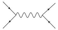
Figure 3: Generic topology of 5D diagrams that give rise to the four-fermion operators upon integrating out the exchanged particle. External states can be doublets or singlets. Consequently the intermediate boson can be a B or Z_X or the SU(2) $W$ gauge boson, if all external states are doublets. Due to the chirality of the external states the fifth component of the boson cannot propagate.

The Wilson coefficient of the four-lepton operator $\left(\bar{L}_{i}\gamma_{\mu}L_{i}\right)\left(\bar{E}_{j}\gamma^{\mu}E_{j}\right)$ is given by

$$b^{LE}_{ij}=\frac{Y_{L}Y_{E}}{4}\left[{g^{\prime}}^{2}\left(b_{0}+b_{1}(c_{L_{i}})+b_{1}(-c_{E_{j}})+b_{2}(c_{L_{i}},c_{E_{j}})\right)+(g^{2}-{g^{\prime}}^{2})\,b_{2}(c_{L_{i}},c_{E_{j}})\right]$$ (43)

with

$$b_{0}=-\frac{1}{4}\,\frac{1}{\ln(1/\epsilon)}\,,$$ (44)

$$b_{1}(c)=-\frac{1}{4}\,\frac{(5-2c)(1-2c)}{(3-2c)^{2}}\,\frac{\epsilon^{2c-1}}{1-\epsilon^{2c-1}}\,,$$ (45)

$$b_{2}(c_{L},c_{E})=-\frac{1}{2}\,\frac{(1-2c_{L})(1+2c_{E})(3-c_{L}+c_{E})}{(3-2c_{L})(3+2c_{E})(2-c_{L}+c_{E})}\,\ln\frac{1}{\epsilon}\,\frac{\epsilon^{2c_{L}-1}}{1-\epsilon^{2c_{L}-1}}\,\frac{\epsilon^{-2c_{E}-1}}{1-\epsilon^{-2c_{E}-1}}\,.$$ (46)

As in [15] we drop terms suppressed by the tiny ratio $\epsilon=T/k$. The result for the minimal RS model can be obtained from this expression by setting the coupling to the $Z_{X}$ to zero, which corresponds to removing the $({g^{2}-{g^{\prime}}^{2}})$ term in (43). Using these expressions the Wilson coefficient of the operator $\left(\bar{E}_{i}\gamma_{\mu}E_{i}\right)\left(\bar{E}_{j}\gamma^{\mu}E_{j}\right)$ takes the form

$$b^{EE}_{ij}=\frac{Y_{E}}{2Y_{L}}b^{LE}_{ij}(c_{L_{i}}\to-c_{E_{i}})\,.$$ (47)

Here and above $Y_{E}$ and $Y_{L}$ are the hypercharges of singlet and doublet lepton field, respectively. For the operator $(\bar{L}_{i}\gamma^{\mu}L_{j})(\bar{L}_{k}\gamma_{\mu}L_{l})$ there are contributions from abelian $Z_{X}$ or $B$ bosons as above, and additionally from the exchange of a $W$ boson. The abelian contribution due to $Z_{X}$, $B$ exchange is given by

$$b^{LL}_{ijkl,{\text{B+Z}}} =\frac{Y_{L}}{2Y_{E}}\,\delta_{ij}\delta_{kl}\,b^{LE}_{ik}(c_{E_{k}}\to-c_{L_{k}})\,\qquad\mbox{(no sum over $i$, $k$)}$$ (48)

The non-abelian bosons generate the operator $\left(\bar{L}_{i}\tau^{A}\gamma^{\mu}L_{i}\right)\left(\bar{L}_{j}\tau^{A}\gamma_{\mu}L_{j}\right)$, which is not part of our basis, and has to be rewritten using the SU(2) Fierz identity

$$\left(\bar{L}_{i}\tau^{A}\gamma^{\mu}L_{i}\right)\left(\bar{L}_{j}\tau^{A}\gamma_{\mu}L_{j}\right)=2\left(\bar{L}_{i}\gamma^{\mu}L_{j}\right)\left(\bar{L}_{j}\gamma_{\mu}L_{i}\right)-\left(\bar{L}_{i}\gamma^{\mu}L_{i}\right)\left(\bar{L}_{j}\gamma_{\mu}L_{j}\right)\,.$$ (49)

We then find the Wilson coefficient of $(\bar{L}_{i}\gamma^{\mu}L_{j})(\bar{L}_{k}\gamma_{\mu}L_{l})$ to be

$$b^{LL}_{ijkl} = b^{LL}_{ijkl,{\text{B+Z}}}+\frac{g^{2}}{4}\left(b_{0}+b_{1}(c_{L_{i}})+b_{1}(c_{L_{j}})+b_{2}(c_{L_{i}},-c_{L_{j}})\right)\delta^{il}\delta^{kj}$$ (50)

$$-\,\frac{g^{2}}{8}\left(b_{0}+b_{1}(c_{L_{i}})+b_{1}(c_{L_{k}})+b_{2}(c_{L_{i}},-c_{L_{k}})\right)\delta^{ij}\delta^{kl}\,.$$

The Wilson coefficients of the seven quark-lepton four-fermion operators are even simpler to compute as there are never two identical fields and all operators but one, $\left(\bar{L}_{i}\gamma^{\mu}\tau^{A}L_{j}\right)\left(\bar{Q}_{k}\tau^{A}\gamma_{\mu}Q_{l}\right)$, are generated via the exchange of an abelian gauge boson. The result is

$$b^{\ell q}_{ij} = \frac{Y_{\ell}Y_{q}}{4}{g^{\prime}}^{2}\Big{[}b_{0}+b_{1}(s_{\ell}c_{\ell_{i}})+b_{1}(s_{q}c_{q_{j}})+b_{2}(s_{\ell}c_{\ell_{i}},-s_{q}c_{q_{j}})\Big{]}$$ (51)

$$+\frac{Y_{\ell}Y^{X}_{q}}{4}\,(g^{2}-{g^{\prime}}^{2})b_{2}(s_{\ell}c_{\ell_{i}},-s_{q}c_{q_{j}})$$

$$b^{L\tau Q}_{ij} = \frac{g^{2}}{4}(b_{0}+b_{1}(c_{Q_{j}})+b_{1}(c_{L_{i}})+b_{2}(c_{L_{i}},-c_{Q_{j}}))$$ (52)

with $\ell\in(L,E)$ and $q\in(Q,U,D)$. $s_{f}$ is $-1$ for a singlet fermion $f$ and $+1$ for a doublet, $Y_{f}$ is the hypercharge of fermion $f$, and $Y^{X}_{q}=T_{R}^{3}-4\tan^{2}\Theta_{W}/(3(1-\tan^{2}\Theta_{W}))$ with $T_{R}^{3}=\{-1,-2,0\}$ for $q={Q,D,U}$. The second line in (51) is only present in the custodially protected model. The dependence on the 5D mass parameters of the quarks shows that muon conversion depends not only on the model parameters of the lepton sector. However, ultimately we only need operators which are built of light quarks fields after EWSB, and of these only the quark-flavour diagonal part. Since both the up- and the down-quark sector masses are hierarchical, the RS Froggatt-Nielsen mechanism generates hierarchical flavour rotation matrices in the quark sector (see e.g. [49]). Consequently, the $b_{2}(c_{x},c_{y})$ terms—the only terms that are simultaneously sensitive to 5D quark parameters and contribute to the flavour-non-diagonal lepton couplings—are suppressed for light quarks, and we neglect them. The only unsuppressed sources of LFV are then the terms $b_{1}(c_{L_{i}})$ or $b_{1}(-c_{E_{i}})$.

3.2.2 Higgs-Fermion operators

The tree-level matching coefficients of the Higgs-fermion operators $\Phi^{\dagger}i\!\overleftrightarrow{D}^{\!\mu}\Phi\,(\bar{\psi}_{i}\gamma_{\mu}\psi_{j})$ follow from the diagrams in Figure 4, where the ones with an external gauge field are related to those without by gauge invariance.

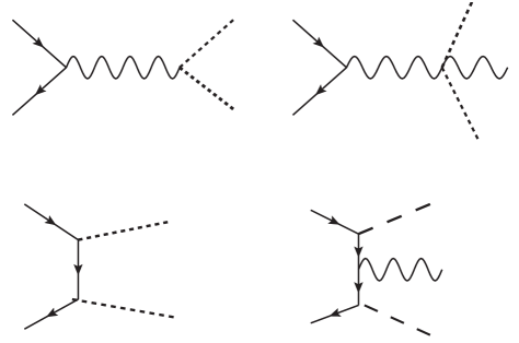
Figure 4: Generic topologies that contribute to operators of the type $\Phi^{\dagger}i{D}_{\mu}\Phi\,(\bar{\psi}_{i}\gamma_{\mu}\psi_{j})$. External fermion states can be either $E$ or $L$. Intermediate and external gauge bosons can be abelian or non-abelian, the external Higgses are indicated by dashed lines.

The diagrams in the first row of Figure 4 have already been computed in [15, 17] for the minimal and custodial RS model. Their contribution to the Wilson coefficients $c^{a}_{ij}=c^{a}_{i}\delta_{ij},\;a=1,2,3$ is given by

$$c^{1}_{i} = \frac{{g^{\prime}}^{2}Y_{E}}{8}\,\Bigg{(}1-\frac{1}{\ln 1/\epsilon}-\left[\frac{(1+2c_{E_{i}})(5+2c_{E_{i}})}{(3+2c_{E_{i}})^{2}}-\frac{2(1+2c_{E_{i}})\ln 1/\epsilon}{(3+2c_{E_{i}})}\right]\frac{\epsilon^{-2c_{E_{i}}-1}}{1-\epsilon^{-2c_{E_{i}}-1}}\Bigg{)}$$ (53)

$$+\,\frac{(g^{2}-{g^{\prime}}^{2})Y_{E}}{4}\left[\frac{(1+2c_{E_{i}})\ln 1/\epsilon}{(3+2c_{E_{i}})}\right]\frac{\epsilon^{-2c_{E_{i}}-1}}{1-\epsilon^{-2c_{E_{i}}-1}}\,,$$

$$c^{2}_{i} = \frac{{g^{\prime}}^{2}Y_{L}}{8}\,\Bigg{(}1-\frac{1}{\ln 1/\epsilon}-\left[\frac{(1-2c_{L_{i}})(5-2c_{L_{i}})}{(3-2c_{L_{i}})^{2}}-\frac{2(1-2c_{L_{i}})\ln 1/\epsilon}{(3-2c_{L_{i}})}\right]\frac{\epsilon^{2c_{L_{i}}-1}}{1-\epsilon^{2c_{L_{i}}-1}}\Bigg{)}$$ (54)

$$+\,\frac{(g^{2}-{g^{\prime}}^{2})Y_{L}}{4}\left[\frac{(1-2c_{L_{i}})\ln 1/\epsilon}{3-2c_{L_{i}}}\right]\frac{\epsilon^{2c_{L_{i}}-1}}{1-\epsilon^{2c_{L_{i}}-1}}\,,$$

$$c^{3}_{i} = \frac{g^{2}}{8}\,\Bigg{(}1-\frac{1}{\ln 1/\epsilon}-\left[\frac{(1-2c_{L_{i}})(5-2c_{L_{i}})}{(3-2c_{L_{i}})^{2}}-\frac{2(1-2c_{L_{i}})\ln 1/\epsilon}{3-2c_{L_{i}}}\right]\frac{\epsilon^{2c_{L_{i}}-1}}{1-\epsilon^{2c_{L_{i}}-1}}\Bigg{)}\,.$$ (55)

As in the case of the four-fermion operators the minimal RS model results can be obtained by removing the terms proportional $(g^{2}-{g^{\prime}}^{2})$. The Wilson coefficients are independent of the Higgs localization provided the limit $\beta\to\infty$ is taken in the bulk Higgs case.

The diagrams in the second row of Figure 4 also exist, but it turns out that they are numerically small compared to the previous contribution. Hence, we only give the explicit expression for the minimal RS model:

$$\delta c^{1}_{ij}= \;-\frac{T^{8}}{k^{8}}\,g_{E_{i}}(1/T)g_{E_{j}}(1/T)F(c_{{L}_{k}})\,Y^{\dagger}_{ik}Y_{kj}$$ (56)

$$\delta c^{2}_{ij}= \;\delta c^{3}_{ij}=\frac{1}{2}\frac{T^{8}}{k^{8}}\,f_{L_{i}}(1/T)f_{L_{j}}(1/T)F(-c_{{E}_{k}})\,Y_{ik}Y^{\dagger}_{kj}$$ (57)

with

$$F(c)=-\frac{k^{4}}{T^{5}}\,\frac{(1+2c)+(3-2c)\epsilon^{2-4c}-(1+2c)(3-2c)\epsilon^{1-2c}}{(1+2c)(3-2c)(1-\epsilon^{1-2c})^{2}}\,.$$ (58)

A similar expression is found in the custodially protected model. The smallness of this contribution arises from the zero-mode profiles of the light external leptons. We ignore the Yukawa contributions $\delta c^{a}_{ij}$ in the subsequent analysis.

3.2.3 Yukawa-type operators

The dominant contribution to the Wilson coefficient of the dimension-six Yukawa-like operators $(\Phi^{\dagger}\Phi)\bar{L}_{i}\Phi E_{j}$ is generated by diagrams of the type shown in Figure 5. In the minimal RS model there is only one diagram as the two intermediate fermions must be a doublet and a singlet lepton. In the custodially protected model both triplet fermions, $T_{3}$ and $T_{4}$, can substitute the singlet. The contribution to the Wilson coefficient is then given by

$$h_{ij} =\frac{N_{cs}}{3}\times\frac{T^{3}}{k^{4}}f^{(0)}_{L_{i}}(1/T)[YY^{\dagger}Y]_{ij}g^{(0)}_{E_{j}}(1/T)$$ (59)

where $N_{cs}$ equals one in the minimal and two in the custodially protected model.

Figure 5: Diagram topology that gives the dominant contribution to the operator $(\Phi^{\dagger}\Phi)\bar{L}_{i}\Phi E_{j}$.

For completeness we remark that the diagrams in the second line of figure 4 also contribute to the Wilson coefficient of $(\Phi^{\dagger}\Phi)\bar{L}_{i}\Phi E_{j}$ through derivative terms that can be eliminated by the fermion equation of motion, such as $\not{D}L_{i}=y_{ij}\Phi E_{j}$. In the minimal model we find

$$\delta h_{ij}=- \frac{1}{2}\,\frac{T^{8}}{k^{8}}g_{E_{l}}(1/T)g_{E_{j}}(1/T)F(c_{{L}_{k}})y_{il}Y^{\dagger}_{lk}Y_{kj}$$

$$- \frac{1}{2}\,\frac{T^{8}}{k^{8}}f_{L_{i}}(1/T)f_{L_{l}}(1/T)F(-c_{{E}_{k}})Y_{ik}Y^{\dagger}_{kl}y_{lj}\,.$$ (60)

Due to the appearance of the small SM lepton Yukawa matrix $y$ this contribution is tiny. This also holds true in the custodially protected model, and hence in the numerical analysis we neglect this term. However, in studies of flavour violation involving third generation quarks (notably top quarks) the contribution can be sizeable and must be included.

3.3 Loop-induced dipole operators

The dipole operators are generated by genuine 5D one-loop penguin diagrams. We distinguish between two classes of diagrams—those with internal gauge-boson exchange proportional to one Yukawa coupling $Y$ and those with Higgs exchange, which involve three Yukawa couplings. A diagram such as shown in Figure 6 below counts as gauge-boson exchange, since it involves only a single $Y$. As we only need the electromagnetic dipole operator for the LFV processes under consideration, we reduce the number diagrams needed for the one-loop coefficient $a_{ij}$ by imposing that the external gauge boson is a photon. In addition, we set the Higgs doublet in the operators $\bar{L}_{i}\Phi\sigma^{\mu\nu}E_{j}B_{\mu\nu}$, $\bar{L}_{i}\tau^{A}\Phi\sigma^{\mu\nu}E_{j}W^{A}_{\mu\nu}$ to its vacuum expectation value. The complete set of non-vanishing diagrams can be found in [15] for the minimal RS model and in [17] for the custodial RS model.

3.3.1 Internal gauge boson exchange

We start the discussion with the gauge-boson contribution. There are three different regions of 4D loop momentum that have to be distinguished. In the first region all propagators are zero–mode propagators. This is only possible for the diagrams that are already present in the minimal RS model as the additional fields in the custodially protected model do not have massless modes [7]. This region corresponds to a SM contribution and must be removed. As explained in [15] this can be done by subtracting the zero-mode from a single 5D gauge-boson propagator.

When the 4D loop momentum is much smaller than the KK scale $T$ and the loop contains at least one KK mode propagator, this propagator can be contracted to a point. The resulting diagram corresponds to a four-dimensional diagram with an insertion of a higher-dimensional tree-level operator. The leading dimension-six contributions are in one-to-one correspondence with the one-loop matrix elements of the operators considered in the previous subsection.

In the last region the 4D loop momentum is of the order of the KK scale $T$. Only this region contributes to the dipole matching coefficient $a^{A}_{ij}$. We extract this contribution by expanding the propagators in the external momenta. This automatically removes the low-momentum region and prevents double-counting of the insertions of tree operators [15]. As the amplitude of the dipole operator is proportional to $\sigma^{\mu\nu}q_{\nu}$ we only have to expand to linear order in the external momenta. The remaining calculation requires the numerical evaluation of integrals over the modulus of the 4D loop momentum and several bulk coordinate integrals in the interval $[1/k,1/T]$. The complete numerical calculation was performed for the minimal RS model in [15] and for the custodially protected model in [17]. Here we use the results of [17] as the routines used there for the numerical evaluation have been considerably improved compared to [15]. We perform the calculation in 5D $R_{\xi}$ gauge and use the spurious dependence of the numerical result on the gauge-fixing parameter as an additional estimate of the numerical uncertainty. From this we conclude that the numerical accuracy is below $0.1\%$, which translates to an error of about 5% for the flavour-non-diagonal LFV terms after rotation to the standard mass basis. This is sufficient for our purposes.

For completeness we remark that some diagrams induce a scheme-dependence of the dipole coefficient $a^{A}_{ij}$ via finite but IR-sensitive $\varepsilon\times 1/\varepsilon$ terms. This scheme dependence is cancelled by the scheme dependence of the 4D one-loop penguin diagrams with insertions of $\beta^{LE}_{ij}$, $\gamma^{a}_{ij}$ [15].

In principle there could be an additional momentum region. The width of the Higgs localization introduces the new scales $T/\delta$ and $\beta T$ for a delta-localized and a bulk Higgs, respectively. In [16] it was shown that the effect of this additional momentum scale does not contribute to the gauge-boson exchange diagrams for $\delta\to 0$ (or, equivalently, $\beta\to\infty$) when only the Higgs zero-mode is considered. For the bulk Higgs case it still needs to be shown that the contribution of the infinite tower of Higgs KK modes also vanishes for $\beta\to\infty$. To this end let us examine the diagram shown in Figure 6. Up to a constant prefactor it is given by

$$\int\frac{d^{d}l\;l^{2}}{(2\pi)^{d}}\int_{\frac{1}{k}}^{\frac{1}{T}}\!\!\frac{dzdxdy}{k^{13}z^{5}x^{5}y^{3}}\,Y^{\beta}_{ij}f_{L_{i}}^{(0)}(z)f_{E_{j}}^{(0)}(x)\Phi^{(0)}(y)\Delta_{\Phi}^{\rm ZMS}(l,z,y)F^{+}_{L_{i}}(l,x,z)\frac{\partial}{\partial l^{2}}\Delta_{B}^{\rm ZMS}(l,y,x)\,.$$ (61)

For the explicit expressions for the zero-mode subtracted gauge boson propagator $\Delta_{B}^{\rm ZMS}$ and the fermion propagator $F^{+}_{L_{i}}$ we refer to [15]. The Higgs propagator $\Delta_{\Phi}(l,z,y)$, its zero-mode subtracted version $\Delta^{\rm ZMS}_{\Phi}(l,z,y)$, the Higgs zero-mode $\Phi^{(0)}(y)$, and the Yukawa coupling $Y^{\beta}$ are discussed in Appendix A.

Figure 6: Example diagram with internal KK Higgs modes.

We now show that the KK Higgs contribution is ${\cal O}(1/\beta)$ and therefore can be neglected for large $\beta$. The Yukawa matrix $Y^{\beta}$ and zero-mode profile $\Phi^{(0)}(y)$ both scale as $\sqrt{\beta}$. Since the zero-mode profile is localized near the IR brane, the associated 5D coordinate integral over $y$ is effectively restricted to the interval $[(1-1/\beta)1/T,1/T]$ of length $1/(\beta T)$. Hence the $y$ integration introduces a factor of $1/\beta$. The integration over $y$ then compensates the factor $\beta$ from the product $Y^{\beta}\Phi^{(0)}(y)$ independent of the magnitude of the 4D loop momentum $l$. For $l\ll T$ and $l\sim T$, the Higgs propagator scales as $1/\beta$ and, after a change of integration variables from $\{x,y,z\}$ to $\{y,y-z,z-x\}$, one finds that the integrand is dominated by the region where the distance $z-y$ is of the order $1/\beta$ (see also Appendix A.4). Putting all factors together, we conclude that the integrand scales as $1/\beta^{2}$ for small loop momenta, and hence the integral over these momentum regions also vanishes for $\beta\to\infty$. For loop-momenta $l$ of order $\beta T$, we can expand the fermion and boson propagator for large momenta, in which case they become simple and their dependence on the loop momentum can readily be extracted. The Higgs propagator is more complicated, but it can only depend on the scale $\beta T$ and therefore scales as $1/(\beta T)$. We find that the product of all three propagators together with the derivative $\partial/\partial l^{2}$, which counts as $1/(\beta T)^{2}$, compensates the factor $l^{5}\sim(\beta T)^{5}$ from $d^{4}l\,l^{2}\sim dll^{5}$. We are left with the two integrals over $y-z$ and $z-x$. For $l\sim\beta T$ the integrand is exponentially suppressed for $|z-x|>1/l$ and $|y-z|>1/l$, and hence each of the coordinate difference integration regions is effectively restricted to size $1/(\beta T)$. We then find that the total scaling of the integrand in this momentum region is $\propto 1/\beta^{2}$. The integral over $dl$ can only compensate one inverse power of $\beta$ and we conclude that the integral over the region $l\sim\beta T$ vanishes as well for $\beta\to\infty$. For very large loop momentum $l\gg\beta T$ we can expand all propagators. Now all bulk coordinate differences are constrained to be within about $1/l$ ($l$ is now the largest scale) and the 5D Higgs propagator scales as $1/l$. This ensures the convergence of the integral as the integrand vanishes as $1/l^{2}$ for $l\to\infty$. The parameter $\beta$ only enters through the integral over $y$, which is cancelled by Higgs profile and Yukawa coupling, hence the integrand is independent of $\beta$. This universal behaviour allows for a straightforward determination of the contribution of the region $l\gg\beta T$:

$$\int_{\beta T}^{\infty}\frac{dl}{l^{2}}=\frac{1}{\beta T}\;.$$ (62)

Hence the integral over this region vanishes in the large $\beta$ limit. Since this holds in all regions, we conclude that KK Higgs contribution vanishes as $1/\beta$.

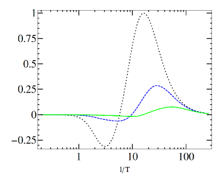
Figure 7: Integrand as a function of the loop-momentum $l$ for $\beta=10$ (black, dotted), $\beta=20$ (blue, dashed) and $\beta=40$ (green, solid). For clarity all curves have been rescaled relative to the maximum of the integrand for $\beta=10$. For loop momenta in excess of $\beta T$ the integrands show a universal $1/l^{2}$ behaviour.

This can be verified numerically as shown in Figure 7. The three curves correspond to different values of $\beta$ (10, 20 and 40, respectively). For better visibility all curves are normalized to the maximum of the $\beta=10$ curve. The maximum of the integrand is close to $l\sim\beta T$ and exemplifies the $1/\beta^{2}$ scaling of the integrand in that region. For large modulus of the (euclidean) loop momentum the three curves lie on top of each other consistent with the $\beta$ independent asymptotic expression. Consequently, the integral over $l$ as well as the contribution to the dipole operator coefficient vanishes for $\beta\to\infty$.

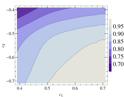
Figure 8: Contour plot of $\mathcal{A}_{ij}$ in the custodially protected RS model normalized to its value for $c_{L}=|c_{E}|=0.7$ as a function of the 5D mass parameters $c_{L}$ and $c_{E}$ for $T=1\,\rm TeV$, $k=2.44\cdot 10^{18}\,$GeV.

To understand the numerical size of the Wilson coefficient $a^{g}_{ij}$ generated by the gauge-boson contribution it is convenient to factorize all terms that combine to the 4D Yukawa matrix before rotation to the mass basis:

$$a^{g}_{ij}=Y_{ij}\frac{T^{3}}{k^{4}}f^{(0)}_{L_{i}}(1/T)g^{(0)}_{E_{j}}(1/T)\mathcal{A}_{ij}=y_{ij}\mathcal{A}_{ij}\;.$$ (63)

The remaining short-distance function $\mathcal{A}_{ij}$ depends only on the 5D bulk masses of the external fermion fields with flavours $i$, $j$ and the RS scales $k$ and $T$. $\mathcal{A}_{ij}$ can be interpreted as a measure of the misalignment between the mass matrix of the lepton sector and the dipole coefficient $a^{g}_{ij}$ before rotation to the mass basis. If the $\mathcal{A}_{ij}$ were all equal, no LFV would be generated by the gauge-boson exchange diagrams. Figure 8 shows the result of the numerical computation of $\mathcal{A}_{ij}$ for the custodially protected model at the KK scale $T=1\,\rm TeV$. There is a small asymmetry in the dependence of $\mathcal{A}_{ij}$ on the bulk mass parameters of the external lepton fields, which arises from 5D diagrams with non-abelian gauge bosons as the $W$ bosons do not couple equally to singlet and doublet fields. To reproduce the 4D lepton mass matrix the bulk mass parameter $c_{L}$ of the doublet muon (electron) has to be around $0.57$ ($0.66$) and the masses of the corresponding singlets around $-0.57$ ($-0.66$), if the SM mass hierarchy is carried by both singlet and doublets. As illustrated in the figure the variation of $\mathcal{A}_{ij}$ in this region is around $\pm(2\text{--}3)\,\%$. In an extreme case where e.g. all singlets are “delocalized” with bulk mass parameter $c_{E}=-0.5$, the bulk mass of the doublet muon (electron) has to be around $0.64$ ($0.8$), and the variation is less pronounced. For the minimal RS model the dependence of $\mathcal{A}_{ij}$ on the bulk mass parameters is slightly smaller in the region of mass parameters relevant to muons and electrons than in the custodially protected model [15, 16]. It follows that the gauge-boson exchange contribution $\alpha^{g}_{ij}$ to the dipole coefficient has smaller off-diagonal elements by a factor 30 to 50 compared to the flavour-conserving diagonal entries—the RS model has a built-in protection from large gauge-boson induced LFV transitions. It is interesting to note that the variation of $\mathcal{A}_{ij}$ increases for decreasing absolute value of both bulk masses. Since typically the absolute values of the 5D bulk masses decrease with decreasing magnitude of the 5D Yukawa couplings, a smaller absolute value of the 5D Yukawa couplings leads to more pronounced LFV transitions from internal gauge-boson exchange.

3.3.2 Internal Higgs exchange

Unlike gauge-boson exchange the internal Higgs-exchange contribution depends strongly on the Higgs localization.

Delta-function localized Higgs

We first consider the delta-function localized Higgs (40). For the minimal RS model the result for a delta-localized bulk Higgs without KK modes was determined in [15] to be

$$a^{H}_{ij}= \phantom{+}\frac{Q_{\mu}e}{192\pi^{2}}\frac{T^{3}}{k^{4}}\cdot\frac{T^{8}}{2k^{8}}\left(F_{L}-F_{E}\right)$$

$$+\frac{Q_{\mu}e}{192\pi^{2}}\frac{T^{3}}{k^{4}}\,f^{(0)}_{L_{i}}(1/T)[YY^{\dagger}Y]_{ij}\,g^{(0)}_{E_{j}}(1/T),$$ (64)

where

$$F_{E}= \hphantom{+}f^{(0)}_{L_{i}}(1/T)Y_{ik}F(-c_{{E}_{k}})Y^{\dagger}_{kh}f^{(0)}_{L_{h}}(1/T)^{2}Y_{hj}g^{(0)}_{E_{j}}(1/T),$$

$$F_{L}= \hphantom{+}f^{(0)}_{L_{i}}(1/T)Y_{ik}g^{(0)}_{E_{k}}(1/T)^{2}Y^{\dagger}_{kh}F(c_{{L}_{h}})Y_{hj}g^{(0)}_{E_{j}}(1/T)\,.$$ (65)

Here the three times repeated indices $k$ and $h$ are summed over only once and the function $F(c)$ is defined in (58). The expression in the first line arises via “off-shell contributions” (see [15, 16]) and is suppressed by fermion zero-mode factors. The last, numerically dominant line (3.3) is not present for the exactly brane-localized setup. As a consequence the Higgs-exchange contribution, which involves three Yukawa matrices, is suppressed in the minimal model with an exactly brane-localized Higgs boson.

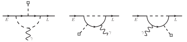
Figure 9: Additional Higgs-exchange diagrams in the custodially protected model.

The corresponding result for the custodially protected model was partially determined in [17]. However, due to a misplaced SU(2) index the two diagram topologies (absent in the minimal model) shown in Figure 9 were missed. These diagrams have a non-trivial dependence on the Higgs localization. In the following we compute these missing diagrams. Note that the exchanged Higgs refers to the zero mode, since for now we have adopted the theta-function regularized delta-function Higgs profile.

To illustrate the computation we consider explicitly the sum of the two right-most diagrams in Figure 9 where the photon couples to the fermion line. Up to prefactors that depend on the U$(1)$ and SU$(2)$ charges of the fermions, and after some simplifications the contribution to the dipole operator structure is given by the integral

$$\mathcal{I}_{new} = \frac{T^{3}}{\delta^{3}}\frac{T^{9}}{k^{12}}\int_{0}^{\Lambda^{2}}\!\!\frac{dl^{2}}{16\pi^{2}}\int^{1/T}_{(1-\delta)/T}\!\!\!\!dx\,dy\,dz\,f^{(0)}_{L_{i}}(x)Y_{ik}Y^{\dagger}_{kh}Y_{hj}g^{(0)}_{E_{j}}(z)$$ (66)

$$\times\,\frac{1}{2}\,\bigg{[}\,\partial_{l^{2}}\Big{(}l^{4}\partial_{l^{2}}\!\left(F_{X_{k}}^{-}(l,x,y)F_{Y_{h}}^{+}(l,y,z)\right)\!\Big{)}+\,l^{2}\partial_{l^{2}}\partial_{l^{2}}\!\left(d^{-}F_{X_{k}}^{+}(l,x,y)d^{-}F_{Y_{h}}^{+}(l,y,z)\right)\bigg{]}\,,\qquad$$

where we used the notation of [15] for the different fermion propagator functions and applied a momentum cut-off $\Lambda$ to the loop integral. The fermion $X$ can be part of the SU(2)_L singlets $\xi_{2},T_{3},T_{4}$ while $Y$ is part of the custodial bi-doublet $\xi_{1}$. Both propagator functions $d^{-}F^{+}$ in the second line obey Dirichlet boundary conditions at $y=1/T$, while the propagator functions $F^{+}$ and $F^{-}$ have Neumann boundary conditions on the IR brane. That is, the second term in square brackets contains wrong-chirality Higgs couplings [13], whereas the first features right-chirality Higgs couplings (correct-chirality in the language of [20]).

Consider first the first term the square brackets in (66). The $l^{2}$ integral can be carried out trivially, since it is a total derivative. Only the upper limit gives a non-zero contribution. Then we use that for $l^{2}\sim\Lambda^{2}\gg T^{2}$ and $x,y$ close to $1/T$, the fermion propagators can be simplified,

$$F^{-}_{X}(l,x,y)\approx F^{+}_{Y}(l,x,y)\propto\frac{i}{l}\cosh(l(1/T-x))e^{l(y-1/T)}\Theta(x-y)+\{x\leftrightarrow y\}\,,$$ (67)

which allows all coordinate integrals to be evaluated analytically. The result is quite involved and depends crucially on the expression $e^{-(\Lambda\delta)/T}$, such that it vanishes for $\Lambda\to\infty$ at fixed, finite $\delta$, but is equal to $1$ for $\delta\to 0$ with fixed $\Lambda$. Hence, for a narrow bulk Higgs (small but finite $\delta$, $\Lambda\to\infty$ first) the first term in square brackets in (66) does not contribute to the dipole Wilson coefficient. This reproduces known results [20, 50] for the right-chirality Higgs couplings. On the other hand, for the exactly brane-localized Higgs, the dipole coefficient receives a finite unsuppressed contribution. This effect is only present in the custodially protected model, since in the minimal model the diagrams do not exist. The contribution of the second term in the square brackets in (66) can be computed following the approach of [16]. Here situation is exactly opposite: the narrow bulk Higgs leads to a finite contribution, whereas the integrals vanish when the Higgs width $\delta$ is taken to zero before the regulator of the loop integral is removed, i.e. for the exactly brane-localized Higgs. The total result is

$$\mathcal{I}_{new}=\left\{\begin{array}[]{rl}\displaystyle\phantom{-}\frac{1}{32\pi^{2}T^{2}}\cdot\frac{T^{3}}{k^{4}}f^{(0)}_{L_{i}}(1/T)[YY^{\dagger}Y]_{ij}g^{(0)}_{E_{j}}(1/T)&\text{``exactly localized''}\\[14.22636pt] \displaystyle-\frac{1}{96\pi^{2}T^{2}}\cdot\frac{T^{3}}{k^{4}}f^{(0)}_{L_{i}}(1/T)[YY^{\dagger}Y]_{ij}g^{(0)}_{E_{j}}(1/T)&\text{``narrow bulk''}\end{array}\right.$$ (70)

The contribution of the left diagram in Figure 9 can be obtained analogously.

Putting all diagrams together and including the SU(2) and hypercharge factors we find in the custodially protected RS model for the narrow bulk Higgs

$$a^{H}_{ij}= \frac{Q_{\mu}e}{192\pi^{2}}\frac{T^{3}}{k^{4}}\cdot 2\cdot f^{(0)}_{L_{i}}(1/T)[YY^{\dagger}Y]_{ij}g^{(0)}_{E_{j}}(1/T)\,,$$ (71)

and for the exactly brane-localized Higgs

$$a^{H}_{ij}= \frac{Q_{\mu}e}{192\pi^{2}}\frac{T^{3}}{k^{4}}\cdot(-3)\cdot f^{(0)}_{L_{i}}(1/T)[YY^{\dagger}Y+Y_{u}Y_{u}^{\dagger}Y]_{ij}g^{(0)}_{E_{j}}(1/T)\,.$$ (72)

In both equations we neglected terms similar to the first line in (3.3), which are suppressed by lepton masses and/or lepton zero-mode profiles. These terms are always subleading in the custodially protected model irrespective of the Higgs localization, and we ignore them in the further analysis. Note that $a^{H}_{ij}$ has opposite signs for the narrow bulk and exactly brane-localized Higgs.

Bulk Higgs with a $\beta$ profile

Figure 10: Example diagram with an internal Higgs exchange and three Yukawa couplings. The internal Higgs can represent the zero-mode or the tower of KK modes.

Next we consider the case of a bulk Higgs with the $\beta$ profile (41). The dominant contributions were studied in some detail in [20] and numerical estimates were obtained by summing a large number of KK modes. Using 5D propagators the effect of the Higgs zero mode can be computed analytically for large $\beta$. To see this let us focus on the simplest diagram, shown in Figure 10. Other contributions can be obtained analogously, but may require appropriate expansions of the fermion propagators for a fully analytic result. For light external fermions the dominant contribution can be written as

$$\mathcal{I}_{H} = Q_{\mu}e\,Y^{\beta}_{ih}\left[Y^{\beta}\right]^{\dagger}_{hk}Y^{\beta}_{kj}\int\frac{d^{4}l}{(2\pi)^{4}}\int_{\frac{1}{k}}^{\frac{1}{T}}\frac{dz\;dy\;dx\;dw}{k^{19}x^{5}y^{4}z^{5}w^{5}}\,f_{L_{i}}^{(0)}(z)g_{E_{j}}^{(0)}(w)d^{-}F^{+}_{L_{k}}(p,x,w)$$ (73)

$$\times\,\Delta_{\Phi}(l,x,z)\Phi^{(0)}(w)\left[d^{-}F^{+}_{E_{h}}(p^{\prime}-l,z,y)F^{+}_{E_{h}}(p-l,y,x)\gamma^{\mu}(\not{p}-\not{l})\right.$$

$$\left.+\,F^{-}_{E_{h}}(p^{\prime}-l,z,y)d^{-}F^{+}_{E_{h}}(p-l,y,x)(\not{p}^{\prime}-\not{l})\gamma^{\mu}\right]$$

where we chose $p,p^{\prime}$ for the incoming and outgoing fermion momentum, respectively. The integral over the $w$ coordinate can be taken right away as we can set $p$ to zero in the external fermion propagator:

$$\mathcal{E}(x,\beta,c_{L},{c_{E}})\equiv\int_{\frac{1}{k}}^{\frac{1}{T}}\frac{dw}{k^{5}w^{5}}\,g_{E}^{(0)}(w)\,d^{-}F^{+}_{L}(p=0,x,w)\,\Phi^{(0)}(w)$$ (74)

$$=i\,\sqrt{\frac{1+2c_{E}}{1-\epsilon^{1+2c_{E}}}}\sqrt{\frac{2(1+\beta)}{1-\epsilon^{2+2\beta}}}\frac{1}{2-c_{L}+c_{E}+\beta}\frac{(Tx)^{2+c_{L}}\epsilon^{-5/2}}{1-\epsilon^{2c_{L}-1}}$$

$$\phantom{=}\times\Big{[}(Tx)^{2-c_{L}+c_{E}+\beta}(1-\epsilon^{2c_{L}-1})+(Tx)^{1-2c_{L}}(\epsilon^{2c_{L}-1}-\epsilon^{1+c_{L}+c_{E}+\beta})-(1-\epsilon^{1+c_{L}+c_{E}+\beta})\Big{]}.$$

After expanding the remaining integrand for small $p,p^{\prime}$ we perform the integral over the photon vertex bulk position $y$ using the completeness and orthogonality relations. We then find

$$\mathcal{I}_{H} = Q_{\mu}eY^{\beta}_{ih}\left[Y^{\beta}\right]^{\dagger}_{hk}Y^{\beta}_{kj}\int\frac{d^{4}l}{(2\pi)^{4}}\int_{\frac{1}{k}}^{\frac{1}{T}}\frac{dz\;dx}{k^{10}x^{5}z^{5}}\,f_{L_{i}}^{(0)}(z)\mathcal{E}(x,\beta,c_{L_{k}},{c_{E_{j}}})\Delta_{\Phi}(l,x,z)$$ (75)

$$\times\,\left[\frac{i}{2}l^{2}\partial_{l^{2}}^{2}d^{-}F^{+}_{E_{h}}(l,z,x)\right](p^{\mu}+{p^{\prime}}^{\mu})\,.$$

This leaves us with only three integrals over $x$, $z$ and the loop momentum.

Let us first consider the Higgs zero-mode contribution by substituting $\Delta_{\Phi}(l,x,z)\to i/l^{2}\times\Phi^{(0)}(x)\Phi^{(0)}(z)$. Since $\beta$ is large but finite until all integrals have been carried out and all regulators removed, we can perform the momentum integral directly in $d=4$ dimensions. To this end, we switch temporarily to the mode picture for the fermion propagator, evaluate the integral

$$\int\frac{d^{4}l}{(2\pi)^{4}}\frac{1}{(l^{2}-m_{n}^{2})^{3}}=-\frac{i}{2(4\pi)^{2}}\frac{1}{m_{n}^{2}}\,,$$ (76)

and resum the mode expansion back into 5D propagators, which results in

$$\mathcal{I}_{H}^{(0)} = -iQ_{\mu}e\,Y^{\beta}_{ih}\left[Y^{\beta}\right]^{\dagger}_{hk}Y^{\beta}_{kj}\int_{\frac{1}{k}}^{\frac{1}{T}}\frac{dz\;dx}{k^{10}x^{5}z^{5}}\,f_{L_{i}}^{(0)}(z)\mathcal{E}(x,\beta,c_{L_{k}},{c_{E_{j}}})\Phi^{(0)}(x)\Phi^{(0)}(z)$$ (77)

$$\times\,\frac{1}{2(4\pi)^{2}}d^{-}F^{+}_{E_{h}}(0,z,x)(p^{\mu}+{p^{\prime}}^{\mu})\,.$$

Since the zero-momentum limit of the fermion propagator has a simple form, the two remaining integrals are elementary. The final analytic expression is lengthy and valid for any positive value of $\beta$. We refrain from giving the explicit expression. However, the limit $\beta\to\infty$ is straightforward. After using (151) to relate the Yukawa matrices for the bulk Higgs to the couplings for the delta-regularized Higgs we recover the same answer as in [15],

$$\mathcal{I}_{H}^{(0)}\to-\frac{iQ_{\mu}e}{96\pi^{2}T^{2}}\frac{T^{3}}{k^{4}}f_{L_{i}}^{(0)}(1/T)Y_{ih}Y^{\dagger}_{hk}Y_{kj}g^{(0)}_{E_{j}}(1/T)\,(p^{\mu}+{p^{\prime}}^{\mu})\,.$$ (78)

This observation is general: the Higgs zero-mode contribution of the bulk Higgs in the $\beta\to\infty$ limit is always equal to the one of the theta-function regularized brane Higgs, see (3.3) and (71). In other words, the localization limit of the bulk Higgs is independent of the bulk profile at finite Higgs localization width.

We still have to determine the contribution from the tower of KK Higgs excitations in the loop. To illustrate the computation in the 5D framework, we consider again the diagram shown in Figure 10. The KK contribution is obtained by the replacement $\Delta_{\Phi}(l,x,z)\to\Delta^{\rm ZMS}_{\Phi}(l,x,z)$ in (75). An analytical evaluation seems difficult even for $\beta\gg 1$. Before turning to the numerical calculation we shall first show that the KK contribution does not go to zero for large $\beta$ despite the fact that the lowest KK masses are of order $\beta T$. This confirms the non-decoupling effect found in [20], now in the 5D framework. To this end we look at the different loop-momentum regions separately. There are two relevant scales, the KK scale $T$ and the Higgs localization scale $\beta T$. This leads to several momentum regions that allow for various expansions of the propagators. The expanded forms can then either be integrated directly or at least their $\beta$ scaling can be determined.

• For small loop momenta $l\ll T$ we can expand both the fermion and the Higgs propagator around $l=0$. We can then analytically integrate the $x$ and $z$ coordinates as in (77). In this region the scaling with $\beta$ must be the same as the scaling of the Wilson coefficient of the four-fermion operator discussed in Section 3.2.1 and in Appendix A.4. That is, for large $\beta$ the integrand scales as $1/\beta$. Hence, the total contribution from this region vanishes for $\beta\to\infty$.

• The second region is $l\sim T$. For the Higgs propagator we can use the same expansion for small euclidean momenta as for $l\ll T$ but the fermion propagator can no longer be expanded. Nonetheless, $d^{-}F^{+}_{E}(l,x,z)$ does not introduce an additional $\beta$ dependence in this momentum region. We recover the overall scaling $\propto 1/\beta$ for fixed values of $l$ just as for $l\ll T$. The only difference to the region with $l\ll T$ is the scaling of the integrand with the loop momentum $l$, which no longer is a simple power law. However, for $l\sim T$, the scaling of the integral with $\beta$ is the same as the integrand, that is $1/\beta$, and hence the contribution from this region also vanishes for $\beta\to\infty$.

• For loop momentum $l$ of the order $\beta T$ we can make use of an expansion of modified Bessel functions of the form $\mathcal{I}_{\beta}(\beta x)$ and $\mathcal{K}_{\beta}(\beta x)$ for large $\beta$, given by

  $$\mathcal{I}_{\beta}(\beta x)\sim\sqrt{\frac{1}{2\pi\beta}}\frac{e^{\beta f(x)}}{(1+x^{2})^{1/4}}\,g(x)\,,\qquad\mathcal{K}_{\beta}(\beta x)\sim\sqrt{\frac{\pi}{2\beta}}\frac{e^{-\beta f(x)}}{(1+x^{2})^{1/4}}\,\tilde{g}(x)\,.$$ (79)

  The exact expressions for the functions $f,\,g$ and $\tilde{g}$ can be found in [51, 52]. Here we only need that $f$, $g$ and $\tilde{g}$ depend on $\beta$ only via terms that vanish at least as fast as $1/\beta$ for $\beta\to\infty$ and that $f(x)$ is a strictly monotonically increasing function of $x$. Using these expansions one can show that the Higgs propagator retains the same $1/\beta$ scaling as in first two regions. Taking into account the behaviour of the fermion propagator for $l\gg T$ we find that $d^{4}l\,l^{2}\,\partial_{l^{2}}^{2}d^{-}F^{+}(l,z,x)$ counts as a factor of $dl\,l$ or equivalently $dl\cdot(\beta T)$. This cancels the $1/\beta$ from the Higgs propagator and leaves us with the coordinate integrals. Their counting is easier to determine when the integral over $w$ has not yet been carried out. The integral over $w$ then cancels the $\sqrt{\beta}$ factors from the Higgs zero-mode profile and one Yukawa coupling. Every integral over a coordinate difference counts as $1/\beta$ (compare the discussion of KK effects in the gauge contribution). Including the two remaining Yukawa couplings, we find that the integrand scales as $1/\beta$ in the region $l\sim\beta T$. Hence the integral over the domain $l\sim\beta T$ takes a constant value for $\beta\to\infty$.

• Finally, for $l\gg\beta T$ we expand the Higgs propagator for large momenta, since it is now dominated by the scale $l$ and no longer by $\beta T$. Consequently, the Higgs propagator scales as $1/l$, and the distance $|x-z|$ is limited to be of order $1/l$. This effectively trades two powers of $1/(\beta T)$ for two powers of $1/l$ compared to result in the $l\sim\beta T$ region, resulting in the scaling $\propto\beta/l^{2}$ of the integrand. The final integral over the modulus of $l$ is therefore convergent and since

  $$\int_{\beta T}^{\infty}\!\!{\rm d}l\;\frac{\beta}{l^{2}}=\frac{1}{T}\,,$$ (80)

  the high-momentum region also gives a finite $\beta$-independent contribution to the dipole operator coefficient.

Since in every region the integral over $l$ either vanishes ($l\ll T$, $l\sim T$) or converges ($l\gg\beta T$ and $l\sim\beta T$) to a constant, the contribution to the dipole Wilson coefficient due to the Feynman diagram in Figure 10 tends to constant for large $\beta$ as announced. For large values of $\beta$ the integral is further dominated by the high-momentum regions and therefore the 5D masses of the fermions enter predominantly via the external zero-modes.

The left panel of Figure 11 shows the numerical result for the integrand as a function of the loop momentum $l$ and demonstrates the expected inversion of the order of the curves for different $\beta$ values from the intermediate to the high-momentum regions. The right panel shows the KK Higgs contribution as a function of $\beta$ normalized to the zero-mode contribution in the $\beta\to\infty$ limit. The plot illustrates the approach of KK contribution to a constant. The relatively fast convergence with increasing $\beta$ is a feature of the simple diagram topology under consideration. The plot shows that the KK Higgs contribution while somewhat smaller than the corresponding zero-mode contribution is of the same order of magnitude [20].

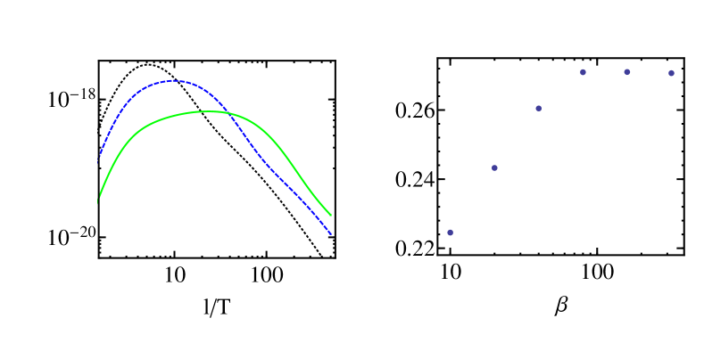
Figure 11: Left: Absolute value of the integrand for the diagram of Figure 10 with zero-mode subtracted Higgs propagator as a function of the loop momentum $l$. The curves correspond to $\beta=10$ black (dotted), $40$ blue (dashed) and $160$ green (solid). The KK scale was set to $T=1\;\rm TeV$. Right: KK Higgs contribution to the dipole operator as a function of $\beta$ normalized to the $\beta\to\infty$ limit of the Higgs zero-mode contribution.

A similar scaling analysis can be applied to all other diagrams involving KK Higgs modes. We will not discuss them in detail, as we have to resort to a numerical evaluation. In Appendix B we give the numerical ratio of the KK tower to the zero-mode contribution for each diagram topology. The final result for dipole operator coefficient generated by the exchange of the KK Higgses is

$$a^{H,\rm KK}_{ij}=\frac{Q_{\mu}e}{192\pi^{2}}\frac{T^{3}}{k^{4}}\cdot\mathcal{A}_{\rm KK}\cdot f^{(0)}_{L_{i}}(1/T)[YY^{\dagger}Y]_{ij}g^{(0)}_{E_{j}}(1/T)$$ (81)

in the minimal model and

$$a^{H,\rm KK}_{ij}=\frac{Q_{\mu}e}{192\pi^{2}}\frac{T^{3}}{k^{4}}\cdot f^{(0)}_{L_{i}}(1/T)\,\big{[}\mathcal{A}^{cs}_{\rm KK}YY^{\dagger}Y+\mathcal{B}^{cs}_{\rm KK}Y_{u}Y_{u}^{\dagger}Y\big{]}_{ij}\,g^{(0)}_{E_{j}}(1/T)$$ (82)

in the custodially protected model, which should be compared to the second line of (3.3) and (71), respectively. Here we again dropped the suppressed “off-shell terms” similar to those in the first line of (3.3). The numerical values of the coefficients are

$$\mathcal{A}_{\rm KK}=0.46(0.04) \mathcal{A}^{cs}_{\rm KK}=1.4(0.2) \mathcal{B}^{cs}_{\rm KK}=0.1(0.05)\,,$$ (83)

where the number in parenthesis shows the estimated error due to the extrapolation to $\beta=\infty$. The sizeable relative uncertainty in $\mathcal{B}^{cs}_{\rm KK}$ comes from large cancellations among the various contributions to the coefficient. In the minimal (custodial) model the KK contribution is about 50% (75%) of the zero-mode contribution.

Irrespective of the Higgs localization, the dipole coefficient $a^{H}_{ij}$ generated by Higgs exchange is in general misaligned relative to the mass matrix. For the bulk Higgs case the numerically dominant terms scale as $YY^{\dagger}Y$ in both the minimal and custodially protected RS model (which includes $Y_{u}Y^{\dagger}_{u}Y$). After rotation to the mass basis this potentially generates large LFV transitions. For the same reason, even after the rotation to the mass basis, unlike the gauge boson contribution, the Higgs contribution depends strongly on the values of the 5D bulk mass parameters and the 5D Yukawa matrices. It usually increases with the magnitude of the Yukawa matrix entries. In the minimal RS model with an exactly brane-localized Higgs, however, $a^{H}$ is much smaller than for the bulk Higgs case (recall that in this scenario only the first line of (3.3) is present).

3.4 Dimension-eight operators

The effects of dimension-eight operators are suppressed relative to the dimension-six ones by a factor of ${\cal O}(v^{2}/T^{2})$ and therefore negligible. However, for LFV observables this counting can be numerically upset, as noted in [14], since the leading dimension-6 contribution to the dipole operator from gauge-boson exchange is suppressed by a factor of 30-50 due to the near-alignment discussed above and in [15, 17] . Relevant dimension-eight effects can arise directly from dimension-eight operators and indirectly from $v^{2}/T^{2}$ corrections to the field rotation to the mass basis.

The first class corresponds to the descendant $(\bar{L}_{i}\sigma^{\mu\nu}E_{i})\Phi X_{\mu\nu}\Phi^{\dagger}\Phi$ ($X=B,W$) of the dimension-six dipole operator $(\bar{L}_{i}\sigma^{\mu\nu}E_{i})\Phi X_{\mu\nu}$, which after EWSB give rise to the same dipole vertex structure. However, the dimension-eight operator has a coefficient function proportional to $YY^{\dagger}Y$ even for the internal gauge-boson exchange contribution, and does not suffer from the alignment suppression of terms proportional to $Y$. Depending on the value of $T$, the dimension-eight contribution may then be the dominant source of flavour violation. This is relevant only for the case of an exactly brane localized Higgs in the minimal RS model, where the contributions to the dimension-six dipole Wilson coefficient cubic in the Yukawa coupling due to Higgs exchange are also suppressed (see previous subsection).

The second class of dimension-eight effects arises from the fact that the tree-level relation

$$\frac{v}{\sqrt{2}}\,U^{\dagger}_{ij}\,\sqrt{\frac{1-2c_{L_{j}}}{1-\epsilon^{1-2c_{L_{j}}}}}Y_{jk}\sqrt{\frac{1+2c_{E_{k}}}{1-\epsilon^{1+2c_{E_{k}}}}}\,V_{kn}=\text{diag}\{m_{e},m_{\mu},m_{\tau}\}$$ (84)

that defines the rotations $U$, $V$ to the mass basis [3] receives corrections due to multiple Higgs vev insertions. The diagonalization condition has the form

$$\frac{v}{\sqrt{2}}U^{\dagger}_{ij}\sqrt{\frac{1-2c_{L_{j}}}{1-\epsilon^{1-2c_{L_{j}}}}}\left[Y-\frac{v^{2}}{6T^{2}}YY^{\dagger}Y\right]_{jk}\sqrt{\frac{1+2c_{E_{k}}}{1-\epsilon^{1+2c_{E_{k}}}}}V_{kn}=\text{diag}\{m_{e},m_{\mu},m_{\tau}\}\,,$$ (85)

cf. (35). The modified $U$ and $V$ field rotation matrices applied to the Lagrangian (3) generate an additional source of LFV which formally enters at the same level in the $v/T$ counting as dimensions-eight operators, which can be taken into account by the substitution

$$a_{ij}^{g}\to a_{ij}^{g}+\frac{v^{2}}{6T^{2}}\left.a_{ij}^{g}\right|_{Y\to YY^{\dagger}Y}$$ (86)

The direct effect of the dimension-eight operators is more difficult to estimate. We have to evaluate the contributions to the dipole-like operators that appear at the dimension eight level, i.e.,

$$\mathcal{L}^{\rm dim-8}\supset\frac{1}{T^{4}}a^{B,\rm dim-8}_{ij}(\bar{L}_{i}\Phi\sigma^{\mu\nu}E_{j})B_{\mu\nu}\Phi^{\dagger}\Phi+\frac{1}{T^{4}}a^{W,\rm dim-8}_{ij}(\bar{L}_{i}\tau^{A}\Phi\sigma^{\mu\nu}E_{j})W^{A}_{\mu\nu}\Phi^{\dagger}\Phi\,.$$ (87)

The computation of the electromagnetic dipole coefficient $a^{\rm dim-8}_{ij}=\cos\Theta_{W}\,a^{B,\rm dim-8}_{ij}-\sin\Theta_{W}\,a^{W,\rm dim-8}_{ij}$ would require the computation of roughly 150 different diagrams in the 5D theory for the minimal RS model alone.

Fortunately, only some of these diagrams actually contribute. For the following we consider only the minimal RS model with an exactly brane-localized Higgs. For the other Higgs localizations the dimension-six dipole is always dominant and dimension-eight terms are negligible as discussed above. We then have two fundamentally different contributions: from the so-called wrong-chirality Higgs couplings (WCHC) and from the ordinary Higgs couplings to lepton modes with the same chirality as the SM zero modes. It turns out that for the exactly brane-localized Higgs the WCHC contribution can be computed analytically and is simply given by

$$a^{\rm dim-8,WCHC}_{ij}=-\frac{1}{3}\left.a_{ij}^{g}\right|_{Y\to YY^{\dagger}Y}$$ (88)

in terms of the dimension-six gauge-boson exchange contribution.

Figure 12: Example of a diagram contributing to the matching onto the dimension-six dipole operator and several related diagrams that contribute to the dimension-eight operator.

To illustrate how this result arises let us consider the left-most diagram in Figure 12 (W8 in the notation of [15]), which contributes to the matching of the $a^{W}_{ij}$ coefficient. There are 10 ways to add two additional external Higgs lines to the fermion line. However, since $\delta/T$ ($\delta$ being the Higgs localization regulator) is much smaller than the dimensional regulator or, equivalently, than the inverse loop momentum cut-off, we find that only the three diagrams shown to the right in Figure 12 give a non-vanishing WCHC contribution for $\delta\to 0$. In each case the integrals over the Higgs vertices can be taken analytically. In the above example the WCHC contributions of the two right-most diagrams cancel, and the remaining diagram can be expressed in terms of the associated dimension-six diagram as shown in (88). Similarly the descendants of all other dimension-six diagrams can be shown to satisfy (88).

Hence the effect of the WCHC can be included via the redefinition

$$a_{ij}^{g}\to a_{ij}^{g}-\frac{v^{2}}{6T^{2}}\left.a_{ij}^{g}\right|_{Y\to YY^{\dagger}Y}$$ (89)

where we used that the Higgs fields will assume their vacuum expectation value ($\Phi^{\dagger}\Phi\to v^{2}/2$). Combining this with (86), we find that the direct and indirect contribution cancel. That is, at the dimension-eight level the WCHCs do not generate sizeable flavour-changing transitions by lifting the misalignment suppression and can be ignored.

This leaves us with the dimension-eight contributions that have no WCHCs. In the minimal model as defined in [15] there are no such contributions from the diagrams with non-abelian vertices. Then there are only seven non-vanishing diagrams that involve an internal $W$ boson, but about 50 diagrams with a hypercharge boson. Fortunately, the limited particle content of the minimal model allows us to recast the expressions of all diagrams in the form of the original dimension-six diagram with modified fermion lines. For instance, the second diagram in Figure 12 has terms without WCHCs, but differs from the original diagram only by the two additional (zero-momentum) Higgs insertions that modify one fermion propagator. This can easily be calculated as the Higgs vertices can be treated analytically. Since the flavour-dependence of the fermion propagators (excluding zero-modes) is relatively mild, one can use the single-flavour approximation, where the Yukawa matrices are the only flavour-dependent quantities. It is then straightforward to compute the contribution to the dimension-eight coefficients. We find

$$a^{\rm dim-8}_{ij}\approx-0.4\left.a_{ij}^{g}\right|_{Y\to YY^{\dagger}Y}\,.$$ (90)

This size is in agreement with the estimate given on the basis of a subset of diagrams in [14], where the non-abelian contribution was found to be $a^{W,dim-8}_{ij}\approx-0.31\left.a^{W}_{ij}\right|_{Y\to YY^{\dagger}Y}$. The minimal model requires a KK scale $T>4\;{\rm TeV}$ in order to pass the constraints set by electroweak precision observables [49]. Hence the dimension eight contribution to $\alpha_{ij}$ is suppressed by an additional factor $v^{2}/T^{2}$ of at least $1/500$. We therefore neglect the contribution of the dimension-eight terms to the off-diagonal elements of $\alpha_{ij}$, since it is smaller than the effect of the Barr-Zee diagrams which also feature three Yukawa couplings without the need to take the dimension-eight term into account.

For the custodially protected model the dimension-eight coefficient would be much harder to compute. Not only does the number of non-trivial Feynman diagram topologies increase significantly, but the larger particle content leads to numerous non-vanishing possibilities to assign the various fermion species to each topology. However, independent of the Higgs localization there always exists an unsuppressed dimension-six contribution proportional to $YY^{\dagger}Y$, hence the dimension-eight terms are never relevant.

4 Phenomenology

The Standard Model in its original form [53] does not allow for flavour violation in the lepton sector. Even after introducing neutrino masses, the charged LFV processes are suppressed by the tiny neutrino masses and too small to be detected in any foreseeable experiment. Any signal of charged LFV is a clear sign of physics beyond the SM. In our analysis of LFV in RS models, we focus on the three processes with the highest current experimental sensitivity, $\mu\to e\gamma$, $\mu\to\bar{e}ee$ and muon conversion in a gold atom. The best current limits for the branching fractions are [56, 54, 55]

$${\rm Br}\left(\mu\to e\gamma\right)<5.7\times 10^{-13}$$ MEG (91)

$${\rm Br}\left(\mu\to\bar{e}ee\right)<1\times 10^{-12}$$ SINDRUM (92)

$${\rm Br}^{\rm Au}\left(\mu N\to eN\right)<7\times 10^{-13} \text{SINDRUM II}\,.$$ (93)

The limit on muon conversion in gold is more stringent than current limits extracted using other nuclei, see e.g., [57, 58] (titanium) or [59] (lead).

In Section 2.2 these three observables were expressed in terms of the Wilson coefficients of the dimension-six SM effective theory Lagrangian, which in turn were determined by integrating out the fifth dimension of the RS model. We now calculate the branching fractions of the observables for a given set of 5D input parameters. Before performing a scan through the parameter space of the model, it is useful to have some qualitative understanding of the effects of the various dimension-six Wilson coefficients. We will generally assume that the 5D Yukawa matrices are anarchic, without imposing any additional flavour symmetries.

4.1 Estimates

We first consider the effect of the dimension-six dipole operator, where we distinguish two different contributions: from the Higgs-exchange diagrams, which involve three Yukawa matrices, and from gauge-boson exchange, which involves only one. The gauge contribution leads to naturally suppressed flavour-violating couplings, whereas the Higgs contribution does not have a built-in flavour protection. For not too small Yukawa couplings the Higgs contribution is dominant. We mainly focus on $\mu\to e$ transitions, for which the dipole coefficients $\alpha_{12}$ and $\alpha_{21}$ are relevant.

To obtain an estimate of the Higgs-exchange contribution let us start with Wilson coefficient [see (71) and (82)]

$$a_{ij}^{H}=\frac{Q_{\mu}e}{192\pi^{2}}\frac{T^{3}}{k^{4}}\cdot f_{L_{i}}^{(0)}(1/T)[(2+\mathcal{A}_{\rm KK}^{cs})YY^{\dagger}Y+\mathcal{B}_{\rm KK}^{cs}Y_{u}Y_{u}^{\dagger}Y]_{ij}g^{(0)}_{E_{j}}(1/T)$$ (94)

in the custodially protected model with a bulk Higgs. An analogous expression holds in the minimal model [(3.3) and (81)]. For an exactly brane-localized Higgs, $a_{ij}^{H}$ is of similar size as above for the custodially protected model, cf. (72), but suppressed in the minimal model due to the absence of the second line of (3.3). Now we recall that the relation of fermion zero-mode profiles, the 5D Yukawa matrix and SM Yukawa matrix (before rotation into the mass basis) is given by

$$y_{ij}=\frac{T^{3}}{k^{4}}\,f^{(0)}_{L_{i}}(1/T)Y_{ij}g^{(0)}_{E_{j}}(1/T)\;.$$ (95)

If the fermion mass hierarchy of the diagonalized SM Yukawa matrix is carried democratically by left- and right-handed fermion modes, i.e.

$$y_{ij}\sim\frac{\sqrt{m_{i}m_{j}}}{v/\sqrt{2}}\,,$$ (96)

we arrive at the estimate

$$a_{ij}^{H}\sim\frac{Q_{\mu}e\sqrt{2m_{i}m_{j}}}{192\pi^{2}v}\left[(2+\mathcal{A}_{\rm KK}^{cs})Y_{\star}^{2}+\mathcal{B}_{\rm KK}^{cs}Y_{u,\star}^{2}\right]\,,$$ (97)

where we assume that

$$Y^{2}_{\star}\equiv\frac{[YY^{\dagger}Y]_{ij}}{Y_{ij}}\quad\qquad Y^{2}_{u,\star}\equiv\frac{[Y_{u}Y_{u}^{\dagger}Y]_{ij}}{Y_{ij}}$$ (98)

are approximately independent of $ij$ (”anarchy”). For anarchic Yukawa matrices we also expect that the rotation matrices $U$ and $V$ follow the same hierarchy $|U_{ij}|\sim|V_{ij}|\sim\mbox{min}\,(\sqrt{m_{i}/m_{j}},\sqrt{m_{j}/m_{i}})$ and hence, barring accidental cancellations, it follows from (9) that $\alpha_{12}=[U^{\dagger}]_{1k}a_{kl}V_{l2}\sim a_{12}$.

Further using that $\mathcal{A}_{\rm KK}^{cs}\approx 1.4\gg\mathcal{B}_{KK}$ we obtain

$$\alpha_{12}^{H}\sim\frac{5Q_{\mu}e\sqrt{m_{e}m_{\mu}}}{192\pi^{2}v}\,Y_{\star}^{2}\,,$$ (99)

which yields

$${\rm Br}\left(\mu\to e\gamma\right)_{|\text{Higgs dipole}}\sim 5\cdot 10^{-9}\times\frac{1\,{\rm TeV}^{4}}{T^{4}}\,{Y_{\star}}^{4}\,.$$ (100)

If the dipole also dominates $\mu\to 3e$ one can combine (13) and (15) to obtain the relation

$$\frac{{\rm Br}\left(\mu\to 3e\right)}{{\rm Br}\left(\mu\to e\gamma\right)}=\frac{2\alpha_{\rm em}}{3\pi}\left[\log\frac{m_{\mu}}{m_{e}}-\frac{11}{8}\right]\approx 0.006\,,$$ (101)

which translates into an estimate of

$${\rm Br}\left(\mu\to 3e\right)_{|\text{Higgs dipole}}\sim 3\cdot 10^{-11}\times\frac{1\,{\rm TeV}^{4}}{T^{4}}\,{Y_{\star}}^{4}\,.$$ (102)

For muon conversion one finds

$${\rm Br^{Au}}\left(\mu N\to eN\right)_{|\text{Higgs dipole}}\sim 1.5\times 10^{-11}\times\frac{1\,{\rm TeV}^{4}}{T^{4}}\,{Y_{\star}}^{4}\,.$$ (103)

We emphasize that these are crude estimates. Even in the anarchic case the random phases of the different elements can lead to cancellations or add coherently. However, they provide useful guidance to the results of the numerical scan discussed below.

The Barr-Zee contribution is similar to the Higgs contribution, since the dominant contribution to the $\eta_{ij}$ Wilson coefficient is also proportional to a product of three Yukawa factors. Comparing the prefactors in (2.2) we find that the Barr-Zee contribution to the dipole coefficient is smaller by a factor of about $170$ than the contribution from the 5D Higgs loops. Thus we expect a $\mu\to e\gamma$ branching fraction of about

$${\rm Br}\left(\mu\to e\gamma\right)_{|\text{BZ}}\sim 2\cdot 10^{-13}\times\frac{1\,{\rm TeV}^{4}}{T^{4}}\,Y_{\star}^{4}\,,$$ (104)

if only the BZ contribution existed. The BZ contribution to the other processes is also smaller by a factor of about $170^{2}$.

Due to the $Y_{\star}^{4}$ dependence the Higgs-exchange induced dipole operator is less important for small Yukawa coupling. In this case, and also for the special case of the brane-localized Higgs in the minimal RS model, the dipole operator generated by gauge-boson exchange becomes crucial. We do not have an analytical expression for the gauge-boson contribution, but we know that there would be no flavour violation from it, if the function $\mathcal{A}_{ij}$ in (63) was independent of $ij$. The 5D mass parameters must decrease with the absolute values of the Yukawa couplings in order to guarantee the correct values for the SM masses fermion masses. $\mathcal{A}_{ij}$ varies more strongly for smaller absolute values of the 5D mass parameters, see Figure 8, and therefore the flavour-changing gauge-boson contribution should increase with decreasing Yukawa coupling. To verify this we fix the Yukawa matrix structure, that is the ratios of all matrix elements, and scale the maximal entry $Y_{\rm max}$ from $2$ to $0.3$. For simplicity we assumed symmetric 5D mass parameters $c_{L_{i}}=-c_{E_{i}}$. The resulting $\mu\to e\gamma$ branching fraction from $a_{ij}^{g}$ alone in the minimal model is shown in Figure 13 (left). The precise value of ${\rm Br}\left(\mu\to e\gamma\right)$ obviously depends on the arbitrarily chosen Yukawa matrix structure, but the variation with the size $Y_{\star}$ of the Yukawa couplings is not very large compared to the fourth-power law of the Higgs-exchange contribution. For the Yukawa matrix used in Figure 13 we find a $\mu\to e\gamma$ branching fraction of a $\text{few}\times 10^{-12}$.

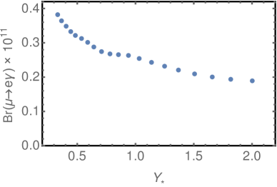
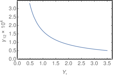
Figure 13: Left: Gauge contribution to ${\rm Br}\left(\mu\to e\gamma\right)$ ($T=1\;\rm TeV$) for fixed Yukawa structure as a function of the absolute Yukawa coupling size. Right: The Wilson coefficient $\gamma_{12}^{1}$ following the approximation (110) as a function of Yukawa coupling size for $T=1\;\rm TeV$. The $\mathcal{O}(m_{\mu}/m_{\tau})$ term is not included.

This agrees with the estimate based on the functional form of the gauge-boson induced dipole coefficient $a^{g}_{ij}$. The numerical value of the Wilson coefficient is [15, 17]

$$a^{g}_{ij}\approx-6\,(19)\cdot 10^{-4}\,y_{ij}.$$ (105)

The value without (in) parenthesis is valid for the minimal (custodial) model and is independent of the details of the Higgs localization. $y_{ij}$ is the 4D Yukawa matrix in the flavour eigenbasis. The matrix relation $a^{g}\propto y$ is only violated by corrections of about (2-3)% as discussed in Section 3.3. This violation is the source of charged LFV as it introduces small off-diagonal elements in the dipole coefficients $\alpha_{ij}$ in the mass eigenbasis after EWSB. Using (96) and applying a factor $2/100$ for the 2% of misalignment between $y_{ij}$ and $a^{g}_{ij}$, we estimate

$$\alpha_{A,12}\sim 2.6\,(8.1)\cdot 10^{-8}\times\frac{2}{100}$$ (106)

for the coefficient relevant to $\mu\to e$ transitions. Again, we regard this as a rough estimate, since there may be cancellations when the rotation into the mass basis is performed. We then find:

$${\rm Br}\left(\mu\to\bar{e}\gamma\right)_{|\text{gauge dipole}} \sim 0.5\,(5)\cdot 10^{-11}\times\frac{1{\rm TeV}^{4}}{T^{4}}$$ (107)

$${\rm Br}\left(\mu\to\bar{e}ee\right)_{|\text{gauge dipole}} \sim 0.3\,(3)\cdot 10^{-13}\times\frac{1{\rm TeV}^{4}}{T^{4}}$$ (108)

$${\rm Br}^{\rm Au}\left(\mu N\to eN\right)_{|\text{gauge dipole}} \sim 0.2\,(2.2)\cdot 10^{-13}\times\frac{1{\rm TeV}^{4}}{T^{4}}$$ (109)

Note that this contribution is independent of the typical size of anarchic Yukawa coupling up to the $\mathcal{O}(1)$ variation shown in Figure 13. It is typically smaller than the Higgs contribution, but provides the “gauge-boson floor” to the dipole coefficient, since it is less sensitive to 5D model parameters than the Higgs contribution and always present. In the custodially protected model the rate is a factor of 10 larger than in the minimal model.

The previous estimates were based on the assumption that the dipole operator dominates the LFV amplitudes. This is not always the case, especially for the $\mu\to 3e$ and muon conversion process. Next, we therefore consider the impact of the four-fermion and fermion-Higgs operators, which are generated at tree-level. In both cases the dimension-six Wilson coefficients are independent of the 5D Yukawa matrices. However, a dependence on the Yukawa matrices enters through the rotation to the mass basis after EWSB. For illustration we consider the operator $(\bar{E}_{i}\gamma^{\mu}E_{j})\,\Phi^{\dagger}i\overleftrightarrow{D_{\mu}}\Phi$ with Wilson coefficient $c^{1}_{ij}=c^{1}_{i}\delta_{ij}$ and restrict ourselves to the minimal model. For all three muon flavour-violating processes the relevant matrix elements are $V^{\dagger}_{1j}c^{1}_{jk}V_{k2}$. Flavour violation arises, because $c^{1}_{i}$ depends on the bulk mass parameter $c_{E_{i}}$, hence $c^{1}_{ij}$ while diagonal is not proportional to the unit matrix in flavour space. We can estimate $V^{\dagger}_{1j}c^{1}_{jk}V_{k2}$ by making use of hierarchical fermion zero-mode functions. Assuming $f_{E_{1}}(1/T)\ll f_{E_{2}}(1/T)\ll f_{E_{3}}(1/T)$ and symmetric mass parameters we can employ the rough estimate $|V_{ij}|\sim{\rm min}\,(\sqrt{m_{i}/m_{j}},\sqrt{m_{j}/m_{i}})$ with $m_{i}$ being the SM lepton masses to obtain

$$\gamma_{12}=V^{\dagger}_{1j}c^{1}_{jk}V_{k2}\sim\sqrt{\frac{m_{e}}{m_{\mu}}}\,(c^{1}_{2}-c^{1}_{1}+\mathcal{O}(m_{\mu}/m_{\tau}))\,.$$ (110)

We can use this formula to study the dependence of $\gamma_{ij}^{a}$ on the size of the 5D Yukawa couplings. Since the product of Yukawa matrix and 5D fermion zero-mode profiles must reproduce the SM mass matrix to leading order in $v/T$, the 5D profiles and therefore the 5D mass parameters are correlated with the Yukawa matrix. The simplest estimate (assuming symmetric mass parameters) yields the correlation $1/\sqrt{Y_{\star}}\sim f^{(0)}_{E_{i}}(1/T)$, where here $Y_{\star}$ is the generic size of the anarchic Yukawa matrix element. In the following we do not distinguish this $Y_{\star}$ from the one defined in (98) for order-of-magnitude estimates. Since the $c^{a}_{i}$ Wilson coefficients arise from a coordinate integral over a single fermion-gauge boson vertex they will roughly scale as $[f^{(0)}_{E_{i}}(1/T)]^{2}$, that is $1/Y_{\star}$. This behaviour was already observed and explained in [13]. The right panel of Figure 13 shows $\gamma^{1}_{12}$ as a function of $Y_{\star}$ (keeping the lepton masses fixed). The curve can be fitted by ${Y_{\star}}^{-0.94}$ confirming the above scaling. This scaling is quite general, although if the mass hierarchy is mainly driven by the right-handed modes, the mass factors in the estimate (110) must change to account for the change in the relation (96).

Similar estimates can be obtained for the four-fermion operator coefficients. Here we have terms with different dependencies on flavour. The Wilson coefficient $b^{LE}_{ij}$ of $(\bar{L}_{i}\gamma_{\mu}L_{i})\,(\bar{E}_{j}\gamma^{\mu}E_{j})$ has three contributions denoted by $b_{0}$, $b_{1}$ and $b_{2}$, see (43). $b_{0}$ does not depend on the 5D masses and hence does not contribute to flavour-changing processes. $b_{1}$ depends on a single bulk mass parameter and has the same scaling $\propto 1/{Y_{\star}}$ as the $c^{a}$ Wilson coefficients. The $b_{2}$ function depends on two bulk mass parameters and scales roughly as $1/{Y_{\star}}^{2}$. However, as discussed below (52), for light leptons this term is suppressed and not relevant. This would be different for processes involving fermions with zero-modes that are IR brane localized such as the (right-handed) top quark, in which case the ratio of exponentials in $b_{2}$ no longer compensates the logarithmic enhancement factor and $b_{2}$ becomes the dominant term in (43).

From (2.2), (22ff) and (27ff) we see that the four-fermion coefficients usually appear in combination with the coefficients of the Higgs-lepton operators. For a typical RS model parameter point, which reproduces the lepton masses, the Higgs-lepton operator coefficients are larger by a factor $\log\epsilon$ relative to the four-fermion operator coefficients. This allows us to use (110) to estimate the effect of the tree-level operators on the generically tree-dominated LFV observables. We find

$${\rm Br}\left(\mu\to\bar{e}ee\right) \sim {\text{few}}\cdot 10^{-12}\times\frac{1{\rm TeV}^{4}}{T^{4}}\,\frac{1}{{Y_{\star}}^{2}}$$ (111)

$${\rm Br}^{\rm Au}\left(\mu N\to eN\right) \sim {\text{few}}\cdot 10^{-9}\times\frac{1{\rm TeV}^{4}}{T^{4}}\,\frac{1}{{Y_{\star}}^{2}}\,,$$ (112)

where we used the parameters given in Table 1. We stress again that these numbers are rough estimates, which depend strongly on the precise structure of the flavour rotation matrices $V$ and $U$. Thus we have three separate contributions to $\mu\to\bar{e}ee$ and muon conversion with different dependence on the size of the 5D anarchic Yukawa coupling ($Y_{\star}^{4}$, $Y_{\star}^{0}$, $Y_{\star}^{-2}$).

$m_{\mu}$	$0.105658$ GeV	[60]	$m_{e}$	$5.10998\cdot 10^{-4}$ GeV	[60]
$s_{W}^{2}$	$0.231$	[60]	$M_{H}$	$125.7$ GeV	[60]
$M_{Z}$	$91.187$ GeV	[60]	$M_{W}$	$80.385$ GeV	[60]
$m_{t}$	$173$ GeV	[60]	$\Gamma_{\mu}$	$2.99598\cdot 10^{-19}$ GeV	[60]
$\mathcal{D}[\text{Au}]$	$0.189$	[35]	$\mathcal{S}^{p}[\text{Au}]$	$0.0614$	[35]
$\mathcal{S}^{n}[\text{Au}]$	$0.0918$	[35]	$\mathcal{V}^{p}[\text{Au}]$	$0.0974$	[35]
$\mathcal{V}^{n}[\text{Au}]$	$0.146$	[35]	$\Gamma^{\text{Au}}_{\text{capture}}$	$8.71\cdot 10^{-18}$ GeV ⋆	[61, 62]
$\mathcal{D}[\text{Al}]$	$0.0362$	[35]	$\mathcal{S}^{p}[\text{Al}]$	$0.0155$	[35]
$\mathcal{S}^{n}[\text{Al}]$	$0.0167$	[35]	$\mathcal{V}^{p}[\text{Al}]$	$0.0187$	[35]
$\mathcal{V}^{n}[\text{Al}]$	$0.0173$	[35]	$\Gamma^{\text{Al}}_{\text{capture}}$	$4.64\cdot 10^{-19}$ GeV	[62]
$f^{u}_{V_{p}}$	$2$		$f^{d}_{V_{p}}$	$1$
$f^{u}_{V_{n}}$	$1$		$f^{d}_{V_{n}}$	$2$
$f^{u}_{p}$	$0.018$		$f^{d}_{p}$	$0.034$
$f^{u}_{n}$	$0.016$		$f^{d}_{n}$	$0.038$
$f^{s}_{n}$	$0.043$		$f^{s}_{n}$	$0.043$

Table 1: Input parameters for the numerical analysis. For the couplings of scalar quark currents to the nucleons we use the results of [36] and fix the value of the nucleon-pion $\sigma$-term to $50\;\rm MeV$. The ^⋆ indicates that we use the average of the values given in the references.

4.2 Numerical analysis

In the previous subsection we attempted to give an idea about the size and the relative importance of the various contributions to our three main LFV observables. While such estimates are useful to understand the rough dependence of our results on the input parameters, especially the Yukawa coupling size, they cannot replace a study of the full parameter dependence. To this end we next perform a numerical scan over the “generic” parameter space. We analyze four RS models: the minimal RS model (as defined in [15]) as well as a custodially protected model (as defined in [17]), each with either an exactly brane-localized or a bulk Higgs including its KK excitations in the $\beta\to\infty$ limit. We refer to these models as $\mathcal{M}$-bulk (minimal, bulk), $\mathcal{M}$-brane (minimal, exactly brane-localized), $\mathcal{C}$-bulk (custodial, bulk) and $\mathcal{C}$-brane (custodial, exactly brane-localized).

The 5D input parameters needed for the numerical evaluation of the dimension-six Wilson coefficients are the 5D Yukawa matrices $Y$ (and $Y_{u}$ in the custodially protected model), the 5D bulk mass parameters $c_{\psi}=M_{\psi}/k$ of the leptons and the KK scale $T$. In case of the exactly brane-localized Higgs the wrong-chirality Yukawa couplings can in principle differ from the “standard” correct-chirality Yukawa couplings, but for simplicity we assume them to be equal. The quark flavour parameters would affect our analysis only through suppressed terms, which are omitted (see Section 3).

Since we do not want to give up the idea of “natural” Yukawa matrices, we further assume that the moduli of the complex Yukawa matrix entries are $\mathcal{O}(1)$ and anarchic. To illustrate how the size of the 5D Yukawa matrix entries affects the different observables, we adopt two scan strategies. In both the modulus of the matrix elements is larger than $0.1$, but in the first (second) scan the maximal modulus $Y_{\rm max}$ is bounded by $0.5$ ($3$ for the second). The phases are arbitrary. Further, we require that the measured values of the charged lepton masses are reproduced by the chosen sets of 5D parameters. Contrary to the minimal RS model the custodially protected RS model includes a right-handed neutrino and a Dirac mass term for the neutrinos. Here we only require the neutrino masses to be below 0.1 eV. However, we do not demand that the PMNS matrix is reproduced by the 5D parameter sets, since the precise values of the neutrino masses do not affect charged LFV, and since, as mentioned in the introduction, the explanation of neutrinos masses and mixings is considered to lie outside the present model frameworks, as must obviously be the case for the minimal models. In practice, we randomly generate 5D Yukawa matrices within the above mentioned constraints, and then fix the 5D mass parameters $c_{\psi_{i}}$ such that the correct lepton masses are obtained. For fixed value of the KK scale $T$ and given scan strategy, we generate about $2\cdot 10^{5}$ Yukawa matrices. For each of these we calculate the Wilson coefficients and then the branching fractions of $\mu\to e\gamma$, $\mu\to e$ conversion, $\mu\to 3e$, $\tau\to\mu\gamma$, and $\tau\to 3\mu$. The required low-energy parameters are shown in Table 1. We also added the material constants of aluminium, which serves as the target for the next generation of muon conversion experiments.

4.2.1 Minimal model

The results of our numerical scan through the constrained parameter space are best illustrated in two-dimensional scatter plots, which visualize the typical range of values for the branching fractions and correlations between the observables. It is important to keep in mind that the point densities in these scatter plots should not be used as a measure for the likelihood of the corresponding value in a given model.

Figure 14 shows the values and correlation of the $\mu\to e\gamma$ and $\mu\to 3e$ branching fractions in the minimal RS model for two different values of $T$, $T=4\,{\rm TeV}$ (top) and $T=8\,{\rm TeV}$ (bottom). $T=4\,{\rm TeV}$ is also roughly the lower bound on the KK scale from electroweak precision observables [49]. The left panels correspond to the $\mathcal{M}$-bulk scenario, the right panels to the $\mathcal{M}$-brane case. Each plot shows the results for $Y_{\rm max}=3$ in blue (dark grey) and for $Y_{\rm max}=1/2$ in orange (light grey). The current and expected future experimental upper bounds are shown by solid and dashed lines, respectively.

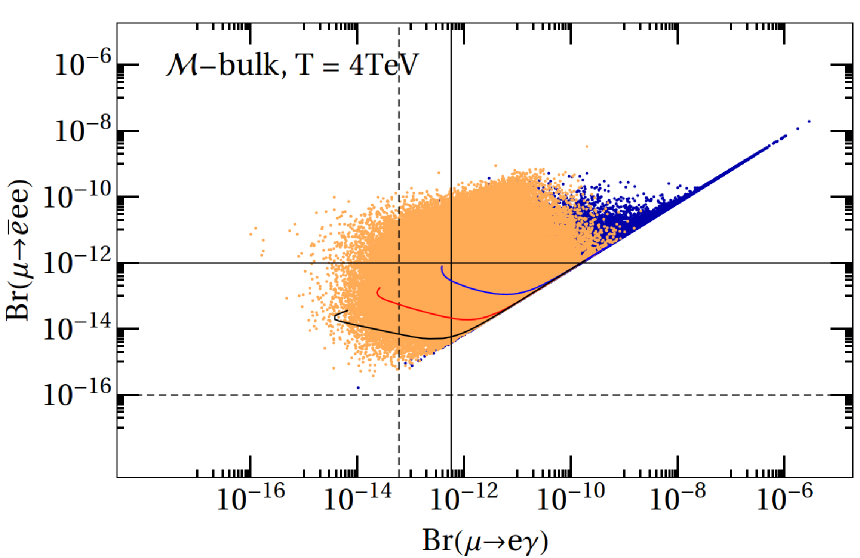
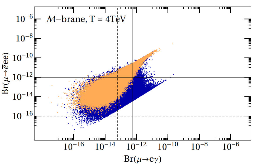
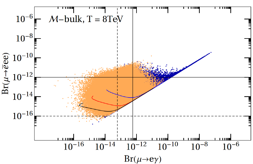
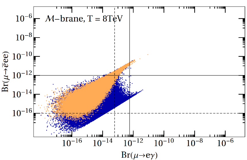
Figure 14: 2D scatter plots of the branching ratios $\mu\to e\gamma$ and $\mu\to 3e$ for fixed $T$ ($4\,{\rm TeV}$ upper row, $8\,{\rm TeV}$ lower row) with $Y_{\rm max}=0.5$ in orange (light grey) and $Y_{\rm max}=3$ in blue (dark grey), respectively. The left panels show the results for the $\mathcal{M}$-bulkmodels, the right panels for the $\mathcal{M}$-brane ones. The current experimental bounds on the branching fractions are given by solid lines. The region above/to the left is excluded. The sensitivity of future experiments is shown by the dashed lines.

All four plots feature a sharp lower bound for $\mu\to 3e$ given the $\mu\to e\gamma$ rate, which is precisely given by the relation (101). $\mu\to 3e$ branching fraction values in the vicinity of this bound are dominated by the contributions from the dipole operator. For very large dipole coefficients or equivalently very large $\mu\to e\gamma$ branching fraction, the tri-lepton decay is always dominated by the dipole, and the two observables are strongly correlated. This generates the prominent thin line directed to the upper-right in the $\mathcal{M}$-bulk model with large Yukawa couplings.

In the bulk Higgs case $\mu\to e\gamma$ is, as expected, quite sensitive to the upper bound $Y_{\rm max}$. This is a consequence of the $YY^{\dagger}Y$ terms in the dipole coefficient. They are naturally flavour-violating and scale with $Y_{\rm max}^{2}$. Consequently, the scan with larger Yukawa entries includes points with substantially larger $\mu\to e\gamma$ branching fraction than the small Yukawa coupling scan. However, the dipole coefficient has two components. While the Higgs and the small Barr-Zee contributions scale as $Y_{\rm max}^{2}$ and vanish when the 5D Yukawa couplings go to zero, the gauge boson exchange contribution is not very sensitive to the Yukawa coupling size. In fact, for a generic anarchic Yukawa it grows mildly with decreasing Yukawa size, see Figure 13. Thus there has to be a smooth transition from the ”Higgs-dominated” to the ”gauge-dominated” regime when the Yukawa coupling decreases.

To illustrate this point we included three curves in the plots for the bulk Higgs case defined as follows. We chose three (random) Yukawa matrices with $Y_{\rm max}=3$ and scale the matrices down to $Y_{\rm max}=0.25$, keeping the relative size of the matrix entries fixed. The curves show the resulting trajectories. For large Yukawa couplings the curves all run close to the dipole dominance bound. With decreasing Yukawa couplings ${\text{Br}}(\mu\to e\gamma)$ and ${\text{Br}}(\mu\to 3e)$ first also decrease following the change in the dipole coefficient. Then the growing effects of the tree-level operators begin to dominate $\mu\to 3e$ and the corresponding branching fraction begins to increase, while ${\text{Br}}(\mu\to e\gamma)$ continues to decrease. For even smaller Yukawa coupling the gauge-boson exchange contribution to ${\text{Br}}(\mu\to e\gamma)$ exceeds the rapidly decreasing Higgs contribution and ${\text{Br}}(\mu\to e\gamma)$ reaches a hard lower limit.

The exactly brane-localized Higgs case displayed in the right panels of Figure 14 behaves the same in this respect. However, since the leading Higgs contribution is suppressed for the exactly brane-localized Higgs, the range of values for ${\rm Br}(\mu\to e\gamma)$ is almost independent of $Y_{\rm max}$. A change in $Y_{\rm max}$ predominantly affects ${\rm Br}(\mu\to 3e)$, which increases for smaller $Y_{\rm max}$ due to the larger coefficients of four-fermion and fermion-Higgs operators. This also explains the drop shape of the scatter plot for $Y_{\rm max}=1/2$. Points with large $\mu\to 3e$ branching fraction arise from large tree-level Wilson coefficients either due to the structure of the Yukawa matrix or due to accidentally small couplings. In both cases the process $\mu\to e\gamma$ also receives sizeable contributions from the tree operators leading to the roughly linear correlation in the upper-right corner of the scatter points.

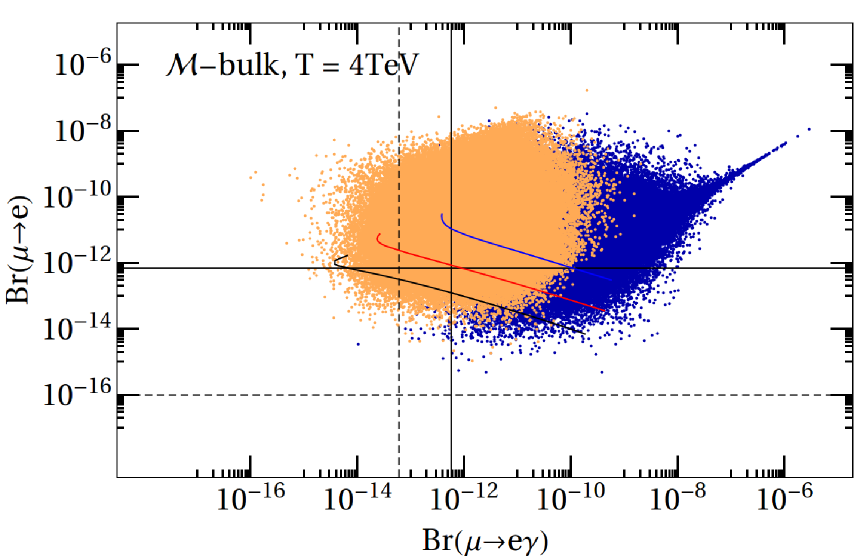
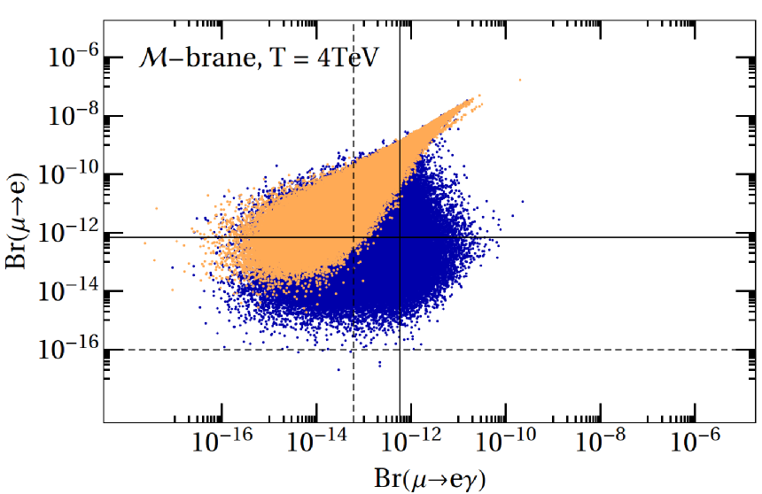
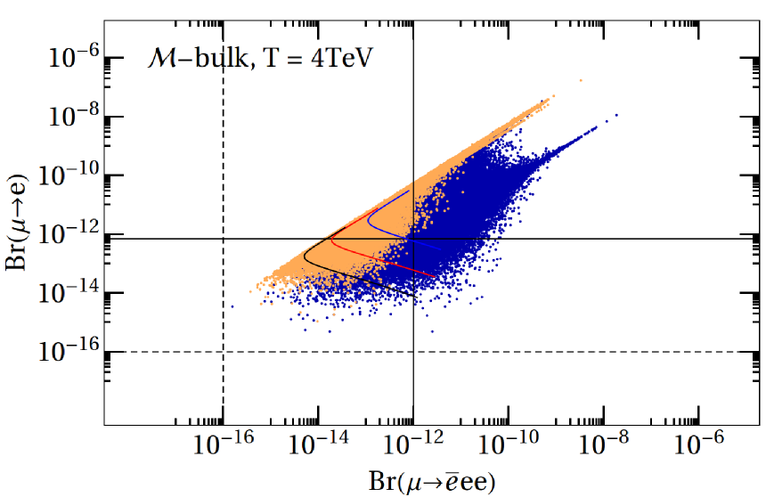
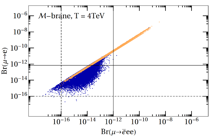
Figure 15: Correlation of the branching ratios for $\mu\to e\gamma$ and $\mu\to e$ (upper row) and for $\mu\to 3e$ and $\mu\to e$ (lower row), both for $T=4\;{\rm TeV}$. The left panels show the results for the $\mathcal{M}$-bulk, the right panels for the $\mathcal{M}$-brane model.

Values and correlations of $\mu\to 3e$ and $\mu\to e\gamma$ with muon conversion in gold are shown in Figure 15 (colour coding as in the previous figure). The top row shows $\mu\to e\gamma$ against $\mu\to e$ ($\mathcal{M}$-bulk left, $\mathcal{M}$-brane right). The two observables are essentially uncorrelated in the bulk Higgs scenario. This agrees with our previous observation that muon conversion is mostly insensitive to the dipole coefficient $a^{A}_{ij}$ which governs the $\mu\to e\gamma$ branching fraction. Only in rare cases is the dipole operator large enough to dominate also muon conversion leading to the noticeable spike towards the right in the upper-left plot. In the exactly brane-localized Higgs case (upper-right panel), correlations are absent only for $Y_{\star}=3$. As mentioned before, for $Y_{\star}=1/2$ $\mu\to e\gamma$ receives non-negligible contributions from tree-level operators, which manifests itself in a weak correlation.

For the same reasons $\mu\to 3e$ and $\mu\to e$ (bottom row) are strongly correlated for small Yukawa couplings in $\mathcal{M}$-brane model, but only feature a lower bound on the branching fraction of $\mu\to 3e$ for a given ${\text{Br}}(\mu\to e)$ in the other scenarios. As noted in the previous subsection, the branching fraction of $\mu\to e$ decreases with increasing values for $Y_{\star}$. This effect can best be seen in the upper left panel of Figure 15. The slopes of the three sample trajectories also verify this effect.

4.2.2 Custodially protected model

Figure 16 shows the combined results for the custodially protected model. The left panels correspond to the bulk Higgs model $\mathcal{C}$-bulk and the right panels to the exactly brane-localized model $\mathcal{C}$-brane. The colour coding is the same as above. Here the KK scale $T$ was fixed to $8\,\rm TeV$, since for $T$ around $4\,{\rm TeV}$ it is already non-trivial to find points, which are not in conflict with the muon conversion bound.

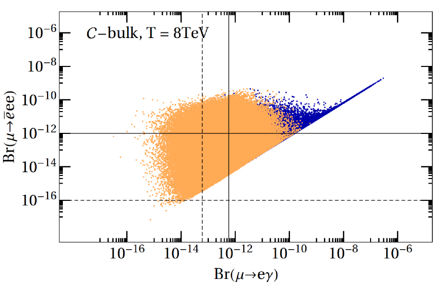
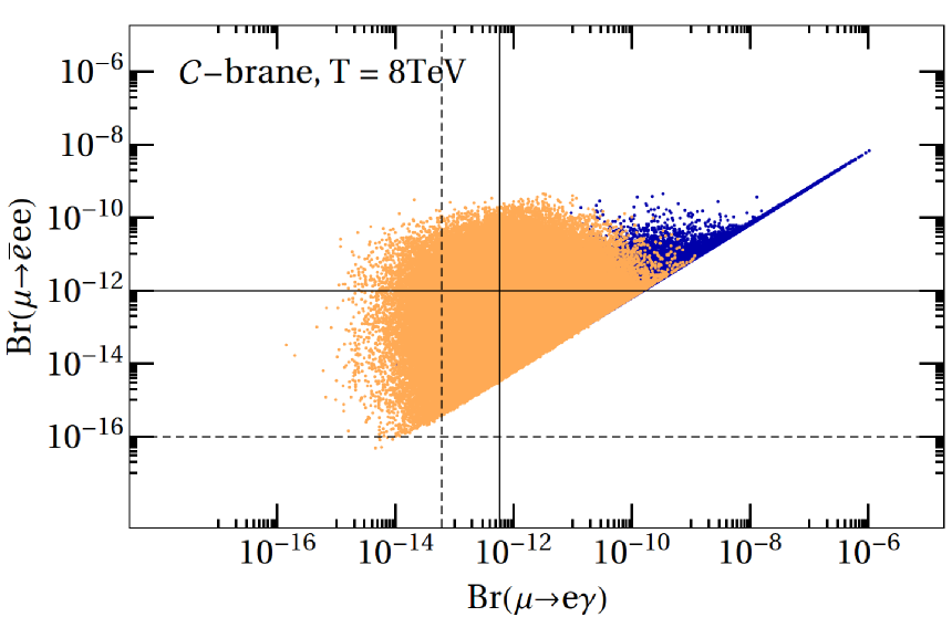
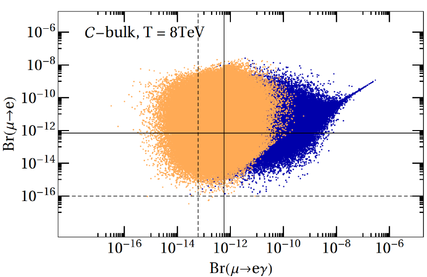
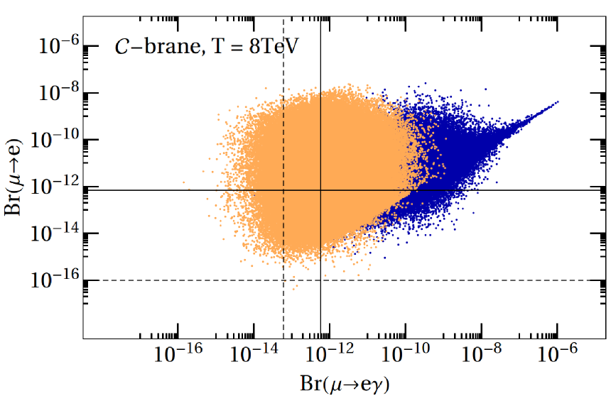
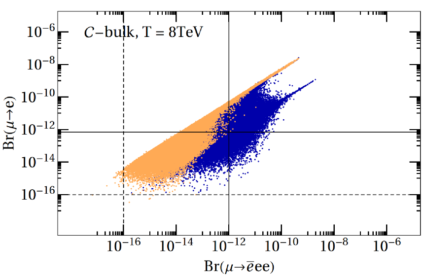
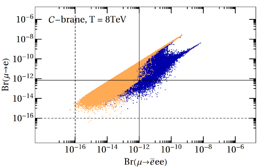
Figure 16: Correlation of the branching ratios for $\mu\to e\gamma$ and $\mu\to 3e$ (top row), $\mu\to e\gamma$ and $\mu\to e$ (middle row), and $\mu\to 3e$ and $\mu\to e$ (bottom row) for $T=8\;{\rm TeV}$ in the custodially protected model. Model points with $Y_{\rm max}=1/2$ are indicated by orange (light grey) points. For $Y_{\rm max}=3$ we use blue (dark grey) points. The left panels show the results for the $\mathcal{C}$-bulk, the right panels for the $\mathcal{C}$-brane model.

The broad picture for model $\mathcal{C}$-bulk is almost the same as for $\mathcal{M}$-bulk. The shape of the distributions does not change. Quantitatively, the custodially protected model generates significantly larger branching fractions. In particular, the $\mu\to e\gamma$ branching fraction, which is most sensitive to the magnitude of the dipole operator coefficient, is typically enhanced by a factor of about five. This was to be expected as the main difference in the custodially protected model is a larger gauge- and Higgs-contribution to the dipole coefficient $a^{A}_{ij}$. Again the dipole operator creates a correlation of $\mu\to e\gamma$ and $\mu\to 3e$ especially for the larger value of $Y_{\rm max}$.

For the $\mathcal{C}$-brane model the distributions are very different from the result in the $\mathcal{M}$-brane model. This is a consequence of the new additional terms (72) in $a^{H}_{ij}$. This additional contribution to the dipole coefficient is only slightly larger than the corresponding contribution for a bulk Higgs. The phenomenology for bulk and brane Higgs case is therefore quite similar in the custodial RS model. The bounds imposed by the non-observation of LFV are comparable, although more restrictive for the exactly brane-localized Higgs.

The fact that the sign of $a^{H}_{ij}$ depends on the Higgs localization does not lead to a noticeable effect. If the dipole operator is dominated by the Higgs contribution, a sign flip of the coefficients $a_{ij}$ only affects terms in (13), (15) and (17) that come from an interference of the dipole with a four-fermion operator. In general, these terms do not provide the dominant contribution to the branching fractions. The situation would be different if the RS contribution could interfere with a sizeable SM contribution to LFV observables. An observed enhanced or reduced rate could then be used to discriminate the brane from the bulk Higgs model.

4.2.3 EDM constraint

The randomly sampled Yukawa matrices also generate electric dipole moments (EDMs) of the leptons through the non-hermitian part of $\alpha_{ij}^{A}$, see (2.1). In case of the electron the relation is given by

$$d_{e}=\frac{Q_{e}e}{2m_{e}}\,F_{3}(0)=m_{e}\,i\,(A_{R}-A_{L})\,,$$ (113)

where the form factor $F_{3}$ now refers to the flavour diagonal electron-photon vertex, and $A_{L,R}$ are defined as in (2.2), (2.2) with subscripts 12 replaced by 11, and $m_{\mu}$ by $m_{e}$.

We checked that the present experimental limit on the electron electric dipole moment [63],

$$|d_{e}|<8.7\cdot 10^{-29}\,e\;\mbox{cm}\quad\mbox{(at 90\% CL)}\,,$$ (114)

does not affect our conclusions. That is, while up to 90% of the randomly scanned model points in the sample with $Y_{\rm max}=3$ (and up to 25% in the $Y_{\rm max}=0.5$ sample) fail the EDM constraint for the bulk Higgs models, the EDM and the LFV observables are uncorrelated, so that the ranges covered by the scatter plots look almost exactly the same, when the points failing the EDM constraint are excluded. Only the tips of some of the spikes pointing to the upper-right in the scatter plots are cut-off in the $Y_{\rm max}=3$ sample, but these points are also excluded by LFV constraints (see solid lines in the previous figures). The predicted values of $|d_{e}|$ and the $\mu\to e\gamma$ branching fraction are shown in Figure 17 for the different RS models and values of $T$ considered in this analysis. The featureless shape of the area filled by the sampled points illustrates the lack of specific correlations. The scaling of both observables with $Y_{\star}$ is visible (orange/light grey vs. blue/dark grey sample) whenever there is an unsuppressed contribution from Higgs exchange.

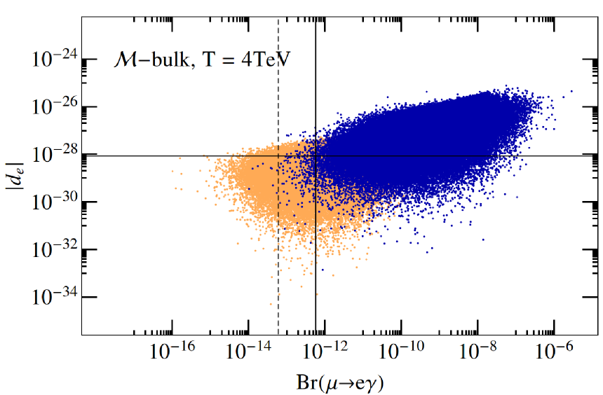
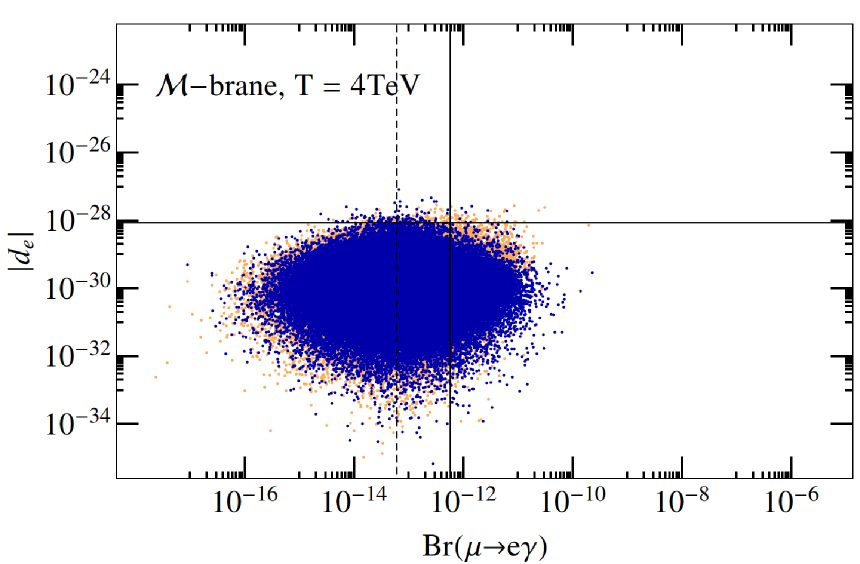
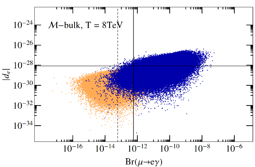
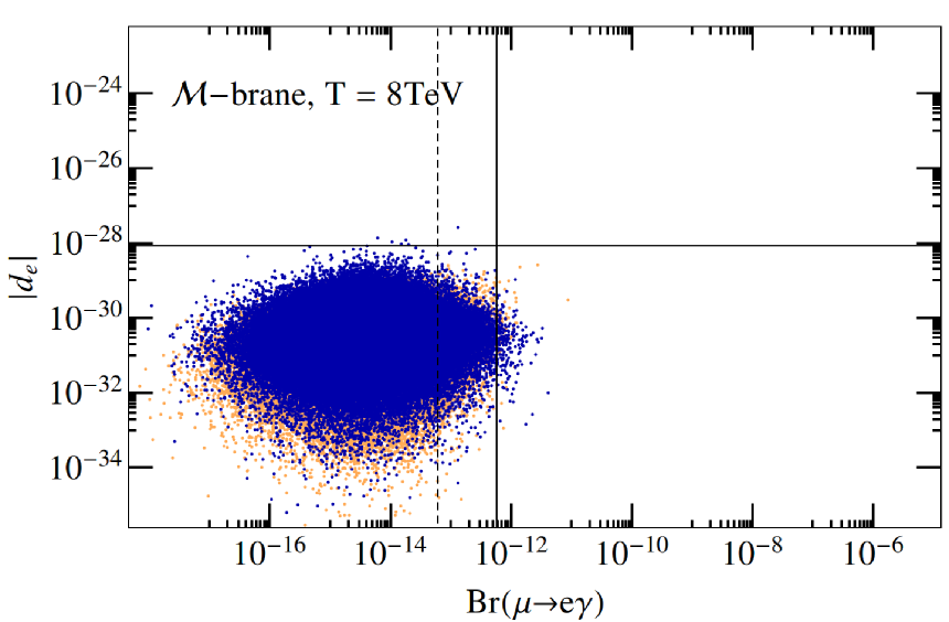
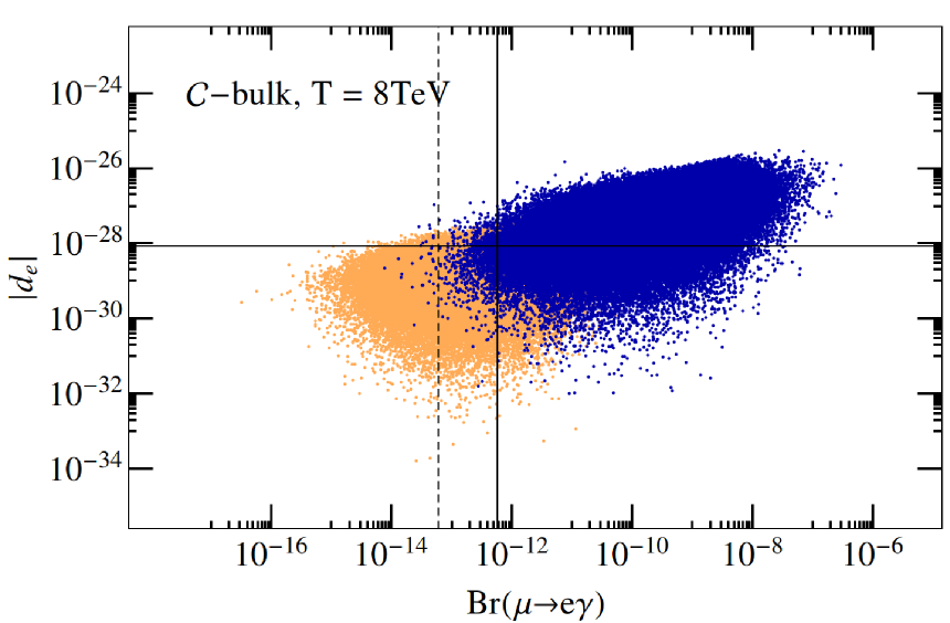
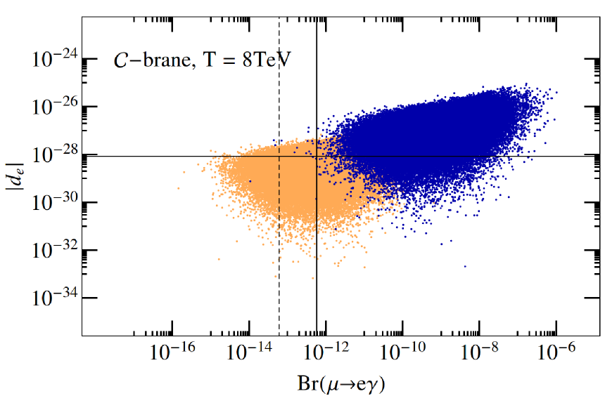
Figure 17: Correlation of the electron EDM with the $\mu\to e\gamma$ branching ratio for all six scenarios. Data sets with $Y_{\star}=1/2$ are indicated by orange (light grey) points. For $Y_{\star}=3$ we use blue (dark grey) points. The left panels show the results for the bulk Higgs, the right panels for the exactly brane-localized Higgs.

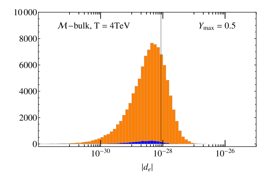
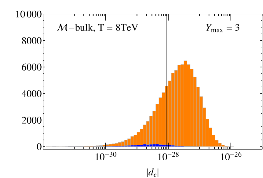
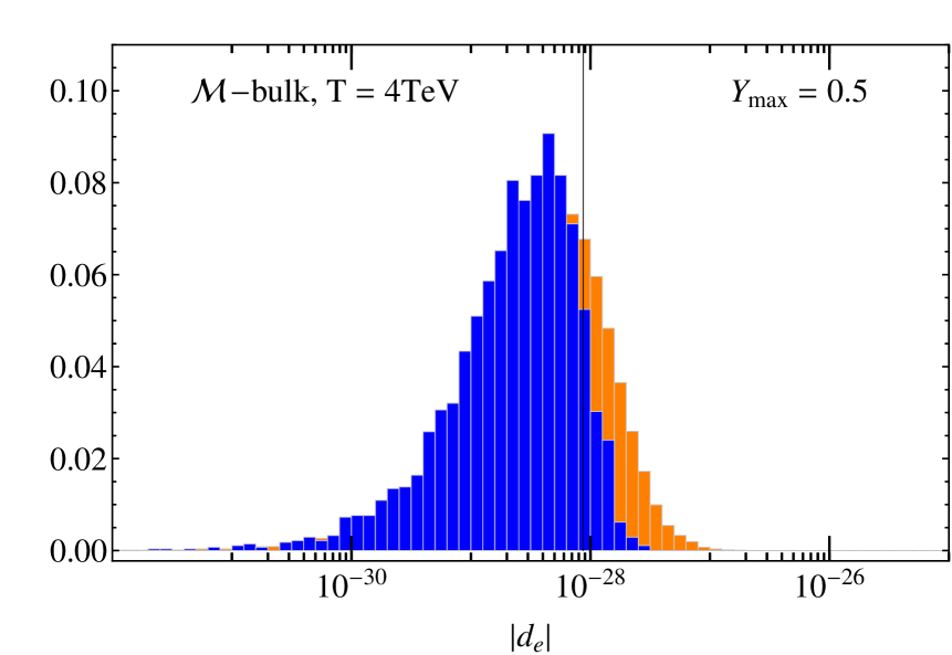
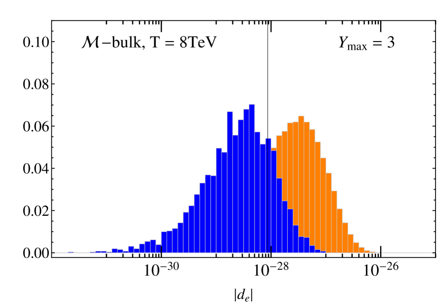
Figure 18: Histograms of the electron EDM distribution of the $\mathcal{M}$-bulk sample before (orange/light grey) and after (darkgrey/blue) the LFV constraints are applied for $T=4\,$TeV, $Y_{\rm max}=0.5$ (left) and $T=8\,$TeV, $Y_{\rm max}=3$ (right). The first row shows the absolute number of representatives of the sample, the second the normalized distribution. The vertical line indicates the current bound (114) on the EDM.

We can turn this question around and ask what are the expectations for value of the electron EDM after the LFV constraints on the RS models are taken into account. To this end we create histograms of $|d_{e}|$ for our samples before and after applying the present  LFV constraints. The $\mathcal{M}$-brane models are special, since the Higgs contribution is strongly suppressed. In these models the EDM distribution peaks at a few times $10^{-30}\,e\;\mbox{cm}$ for $T=4\,$TeV, well below the present limit (114) and is hardly altered by the LFV constraints. The tail of the distribution above about a few times $10^{-29}\,e\;\mbox{cm}$ is, however, cut away independent of the value of the Yukawa coupling. This is different for the other models where the distribution and impact of constraints is sensitive to the maximally allowed Yukawa coupling $Y_{\rm max}$. This is illustrated on the example of the $\mathcal{M}$-bulk model in Figure 18, where the left two panels refer to $T=4\,$TeV, $Y_{\rm max}=0.5$ and the right ones to $T=8\,$TeV, $Y_{\rm max}=3$. The respective upper plot shows the distribution of $d_{e}$ before (light grey/orange) and after (dark grey/blue) the LFV constraints are applied. The second distribution is hardly visible, as most of the models in these two samples are excluded by the LFV constraints. In the second row we therefore show the normalized distribution for the two cases. In the first case, $T=4\,$TeV, $Y_{\rm max}=0.5$ the tail of larger values of $d_{e}$ is cut away, while the peak of the distribution remains at the same value as without the LFV constraints. In the second case, $T=8\,$TeV, $Y_{\rm max}=3$, most of the distribution without LFV constraints lies above the EDM bound (114) indicated by the vertical line. When the LFV constraints are taken into account the expected value of the electron EDM reduces by more than an order of magnitude. We note that with LFV constraints applied the current EDM bound is always close to the upper end of the distribution. In other words, quite generally, the lepton-flavour violating processes put similar generic bounds on the electron EDM as the current bound from the direct EDM measurement. Of course, these conclusions hold in the parameter space of RS models with anarchic Yukawa couplings in a statistical sense, and not for any particular model.

4.3 A note on LFV $\tau$ decays

Tau decays offer another opportunity to study LFV. However, the short lifetime of the $\tau$ and its high mass make it unsuited for studies in low-energy facilities. The best bounds on processes like $\tau\to e\gamma$ or $\tau\to 3\mu$ come from Babar [64], Belle [65] as well as LHCb [66].

The RS model naturally generates higher rates for $\tau\to\mu,e$ transitions than for $\mu\to e$ transitions, since there is a close relation of lepton masses with the corresponding zero-mode profiles, which also control the size of LFV. However, the fantastic sensitivity of past and future experiments searching for muon flavour violation still makes searches in the muon sector the most promising avenue, unless an additional flavour structure suppresses muon flavour violation.

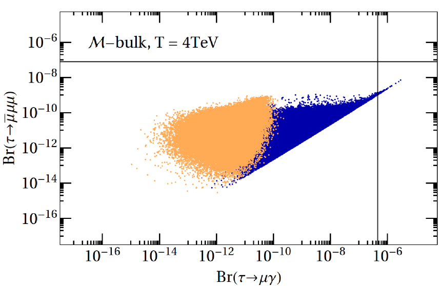
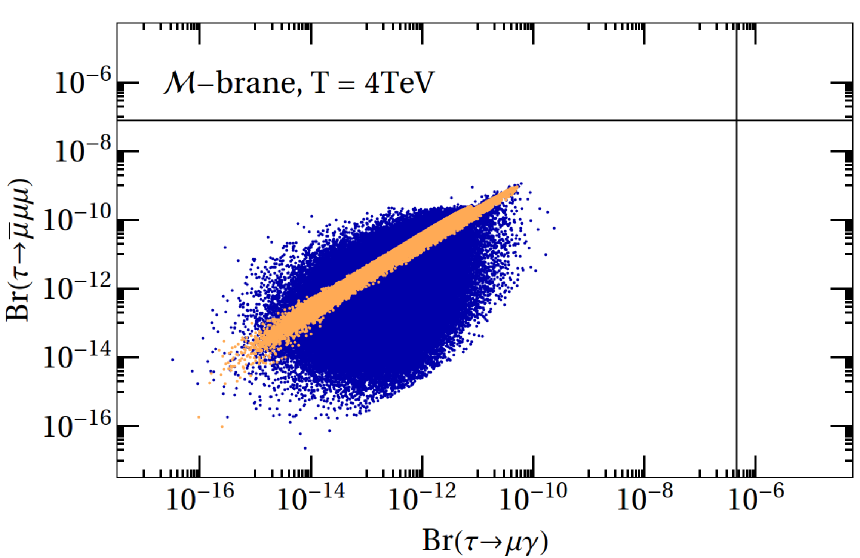
Figure 19: Correlation of the branching ratios of $\tau\to\mu\gamma$ and $\tau\to 3\mu$ for $T=4\,\rm{TeV}$ in the minimal model. The left panel shows the bulk Higgs, the right the exactly brane-localized Higgs case.

Nevertheless, it is instructive to provide the expectations for tau LFV in the RS model. In Figure 19 we show the values and correlation of the $\tau\to\mu\gamma$ and $\tau\to 3\mu$ branching fractions. The colour coding is the same as in the previous subsection. The solid lines correspond to the current best upper bounds on the branching fractions. Compared to the bounds in the muon sector the current limits from tau decays are not restrictive even for $T=4\,{\rm TeV}$. An improvement of more than five orders of magnitude would be required for constraints as severe as those from muon decays.

Qualitatively, the $\tau\to\mu\gamma$ vs. $\tau\to 3\mu$ plot is similar to the corresponding “muonic” plots (first row in Figure 14). The main difference is the large effect of the four-fermion and fermion-Higgs operators. For the exactly brane-localized Higgs this generates the strong correlation for small Yukawa couplings $Y_{\rm max}=0.5$. In the bulk Higgs case this effect prevents scatter points close to the dipole-dominance line.

4.4 Discussion

In the following we summarize and emphasize the main conclusions from the phenomenological study. Based on the topologies of the decays we (naively) expected that $\mu\to e$ conversion in nuclei and $\mu\to 3e$ are driven by the current-current operators $(\bar{\ell}_{e}\Gamma\ell_{\mu})\,(\bar{\psi}\Gamma\psi)$, whose Wilson coefficients are determined by the tree-level four-fermion and Higgs-fermion coefficients, $c_{ij}^{a}$ and $b_{ij}$, in the dimension-six SM effective Lagrangian (3). Whereas the rate for radiative muon decay should primarily be determined by the loop-induced dipole operator. This situation would be ideal, as the two groups of processes would then provide complementary information on the underlying RS model through the different parameter dependencies of the relevant Wilson coefficients.

However, and this is our main message #1, we find that this is not generally the case. In particular, the process $\mu\to 3e$ can receive sizeable contributions from dipole operators. This can even be the dominant effect as indicated by the prominent dipole dominance line in the plots. In the minimal RS model with an exactly brane-localized Higgs and small Yukawa couplings the situation can also be reversed. Then $\mu\to e\gamma$ receives relevant contributions from tree-level coefficients and is no longer governed by the dipole operator alone. This makes it clear that it is necessary to consider all dimension-six operators for every observable to arrive at a reliable picture of LFV in the RS model.

From our numerical analysis we also see that it is important to include both, the Higgs and the gauge-boson exchange contribution to the penguin diagrams that generate the dipole Wilson coefficient $\alpha^{A}_{ij}$, because they exhibit a fundamentally different dependence on the parameters—most notably the Yukawa coupling. Only the full dipole coefficient including all contributions gives an accurate description of the $\mu\to e\gamma$ decay over a large range of Yukawa sizes. Without the Higgs contribution the dominant effect for large Yukawa couplings is completely missed. Whereas the presence of the gauge-boson exchange contribution prevents the dipole from becoming irrelevant for small Yukawa couplings. This manifests itself in a lower bound on ${\rm Br}(\mu\to e\gamma)$, which depends only on the structure of the Yukawa matrix but not on the overall size of the couplings. This is our main message #2: in RS models Higgs and gauge-boson induced flavour violation can both be important and only a full calculation of the dipole operator coefficient gives a reliable picture of LFV over all of the parameter space.

The scans suggest that anarchic RS models with minimal particle content typically need KK scales $T$ larger than $4\,{\rm TeV}$ to be compatible with the current data on charged LFV. For models with a bulk Higgs the combination of $\mu\to e\gamma$ and muon conversion makes the bound on $T$ almost insensitive to the size of the Yukawa matrix. For an exactly brane-localized Higgs the situation is more complicated. $T\gtrsim 4\,\rm TeV$ is still valid for small Yukawa couplings. However, in this model the limit on $T$ comes mainly from muon conversion data. As discussed above, muon conversion is dominated by tree-level operators whose Wilson coefficients decrease for increasing $Y_{\star}$. Thus, the bound on $T$ gets weaker the larger the Yukawa couplings. For $Y_{\rm max}=3$ we can still find numerous data point that satisfy all constraints for $T$ as low as $2\,\rm TeV$. In the custodially protected model on the other hand, the larger particle content generally leads to larger Wilson coefficients. Consequently, the lower bound on admissible KK scales $T$ is higher. It is noteworthy that in the custodially protected model the bound on $T$ is essentially independent of the Higgs localization for all three observables.

The limits on the KK scale $T$ will significantly improve in future experiments. Especially the next generation muon conversion searches will provide strong constraints on RS models. Our analysis was performed for a gold target nucleus—DeeMe [67], Mu2E [68] and COMET [69] use silicon and aluminium target nuclei, respectively. Aluminium and silicon have an approximately $20$ times smaller muon capture rate compared to gold, which enhances the branching fraction, but the wave-function overlap integrals ($\mathcal{D}$,$\mathcal{V}$,$\mathcal{S}$) relevant to muon conversion are also smaller, see Table 1. Thus an expected lower bound on the branching fraction of $7\times 10^{-17}$ for aluminium is roughly equal to a bound around $10^{-16}$ in gold [35] (indicated by the dashed lines in the plots). This combined with the expected improvement on ${\rm Br}(\mu\to e\gamma)$ during the next run of the MEG experiment [70] could exclude the parameter space of anarchic RS models (custodially protected or minimal) up to a lowest KK resonance mass of 20 TeV, which corresponds to $T\gtrsim 8\,\rm TeV$. The current $\mu\to 3e$ constraint is less constraining than the one from muon conversion. However, the proposed Mu3e experiment [71] aims for sensitivity to a branching fraction of about $10^{-16}$. At this level $\mu\to 3e$ alone will be able to exclude anarchic models with $T\lesssim 5\,{\rm TeV}$. Naturally, should LFV be observed in any of the new experiments, the model-dependent correlations among different processes can be used to further constrain the RS parameter space. Hence, our main message #3: LFV violation provides very strong constraints on RS models, and future experiments will further strengthen them.

It is interesting to compare the charged LFV constraints on the RS model and its KK scale to those derived from other processes. The non-observation of direct KK gluon production forces $T$ to be larger than only about $1\,\rm TeV$. This cannot compete with the bounds from electroweak precision observables, notably the $S$ and $T$ parameter, which are essentially model-independent. They only depend on the particle content of the model and to a lesser degree on the 5D Higgs profile [72]. For the two models discussed in this work the electroweak precision observable bounds are $T>2.3\,\rm TeV$ (custodially protected) and $T>4\,\rm TeV$ (minimal) [49]. For not too large Yukawa couplings the RS contribution to $(g-2)_{\mu}$ is model-independent in the same sense [15, 17]. However, in this case the SM contribution is non-zero and given the present situation of experiment and SM theory, the bounds on the KK scale are not competitive.

If one allows for a somewhat stronger dependence of the bounds on the model parameters, Higgs production (and subsequent decay) is also an interesting observable. It depends more strongly on the (mainly quark) Yukawa matrices $Y_{u},Y_{d}$ than the oblique parameters, but is still far less sensitive to its detailed structure than processes like $\mu\to 3e$, because Higgs production depends to leading order only on the traces of $Y_{u}^{\dagger}Y_{u}$, $Y_{d}^{\dagger}Y_{d}$. The trace of a product of anarchic matrices follows a narrower distribution than an individual matrix element. One finds that $T$ has to be larger than $2\,(4)\,{\rm TeV}\;\text{@}\,95\%\,\rm CL$ for $Y_{\star}\approx 3$ in the minimal (custodially protected) model with a narrow bulk Higgs [31]. For smaller Yukawa couplings the bound becomes weaker as the effect on the production cross section decreases with $Y_{\star}$. For the exactly brane-localized Higgs the constraints are stronger, and one finds the same bounds on $T$ as above already for $Y_{\star}\approx 1$. As we have seen the situation is different for LFV observables. In the minimal model an exactly brane-localized Higgs leads to weaker bounds than a bulk Higgs, and in the custodially protected model the bound from the bulk Higgs (with KK modes) is comparable to the one in the exactly brane-localized scenario. Thus for large quark Yukawa couplings and the exactly brane-localized Higgs, Higgs production provides at least equally strong bounds on the KK scale than the non-observation of charged LFV. The LHC will be able to improve on this further in the future. In all other cases the next generation LFV experiments will be able to set the most stringent limits on the KK scale. Of course, this comparison assumes that the magnitude of anarchic Yukawa couplings is roughly the same in the quark and lepton sectors.

The quark-sector Yukawa couplings also enter the RS modification of meson oscillations, where in particular $\epsilon_{K}$, which measures CP violation in kaon mixing, is very sensitive to coloured KK states [8, 9]. If we follow [8] and estimate this effect from the dominant left-right four-quark operator $(Q_{i}\gamma_{\mu}T^{A}Q_{i})(D_{j}\gamma^{\mu}T^{A}D_{j})$ along the lines of Section 4.1, we find that $T$ in excess of $8\,\rm TeV$ is needed to avoid conflict with experimental data. We have seen in the previous section that for any given data point $\mu\to e\gamma$ can differ by orders of magnitude from the simple estimate, since cancellations may or may not be present for a given set of 5D Yukawa and mass parameters. The same is true in the quark sector and much smaller modifications of $\epsilon_{K}$ than indicated by the naive estimate are possible, see [9]. We confirmed this independently using the results of [73]. Thus, from an analysis similar to the one performed in the previous section, as well as from [9], the limit of the TeV brane scale from $\epsilon_{K}$ is around $T=7\,\rm TeV$ — quite close to the one expected from the next generation LFV experiments. However, contrary to $\epsilon_{K}$, whose ultimate reach is limited by the theoretical precision of the SM prediction, the potential of LFV observables, in particular of $\mu\to e$ conversion, is not yet exhausted. In any case, given that the quark and lepton Yukawa couplings may exhibit different patterns, independent tests of the RS model in both the quark and lepton flavour sectors in a wide range of observables are not redundant.

Our findings can be compared to the results of [13], which provided the first detailed analysis of lepton flavour violation in the minimal RS model in the KK mode picture. The branching ratio of $\mu\to e\gamma$ is determined from the Higgs-exchange contribution to the dipole Wilson coefficient alone, which is computed via one-loop diagrams involving the Higgs zero-mode and first fermion KK excitation. Muon conversion and $\mu\to 3e$ are computed from the tree-level Wilson coefficients, while the dipole contribution is neglected. Both exactly brane-localized and bulk Higgs scenarios are investigated. We can compare with our full results only for the bulk Higgs case as their exactly brane-localized Higgs result for the dipole operator is cut-off dependent. Despite these caveats the overall size of the bound on the KK scale $T$ for a bulk Higgs is compatible with the one found above. The main difference is the dependence of the branching fractions on the model parameters. As [13] only includes the Higgs contribution, the dipole coefficient has a straightforward dependence on the Yukawa coupling size $Y_{\star}$. The identification of the dependence on the Yukawa coupling size as a distinguishing feature of tree-level and loop-induced observables, i.e. muon conversion and tri-lepton decay as opposed to $\ell^{\prime}\to\ell\gamma$, is however valid only for medium-size Yukawa couplings, since otherwise the neglected gauge-boson contribution with its different dependence on $Y_{\star}$ becomes relevant for small $Y_{\star}$, and for large $Y_{\star}$ the tri-lepton decay is dominated by the dipole operator and therefore effectively also loop-induced.

We can also compare our results with [14]. Here the Higgs-exchange contribution to the dipole operator is not considered. The dipole coefficient is computed in the 5D framework from a subset of gauge-boson exchange diagrams including a dimension-eight effect with three Yukawa matrices. Comparing orders of magnitudes their results for $\mu\to e\gamma$ and $\mu\to 3e$ are similar to our exactly brane-localized Higgs case in the minimal model. In particular, the lower bound on the $\mu\to e\gamma$ branching fraction for small Yukawa couplings is also present in their estimates.

5 Summary

In this paper we have undertaken a comprehensive study of charged lepton flavour violation in Randall-Sundrum models. The approach follows the strategy developed in [15], that is we assume that the KK scale is significantly larger than the electroweak scale and match the RS theory to the SM effective theory including dimension-six operators by integrating out the extra dimension in a fully 5D quantum-field-theoretical framework. Some of the Wilson coefficients of the dimension-six operators could be taken from [15, 17] and the remaining ones were computed here. We considered the RS model with minimal field content and an extended model with additional fields to protect low-energy precision measurements from custodial symmetry violating contributions. We further considered three implementations of the IR-brane localized Higgs field. The exactly localized case and the limiting cases of a bulk Higgs with and without KK Higgs excitations. The third scenario was motivated by the recent work [20], which demonstrated the non-decoupling of Higgs KK modes in the KK mode picture. We confirm this finding within the 5D framework.

Our calculation is the first complete one of dimension-six effects (more precisely those not suppressed by powers of small lepton masses), and considerably sharpens previous results from [13, 14, 16]. This concerns in particular the Wilson coefficient of the electromagnetic dipole operator $\bar{L}_{i}\sigma^{\mu\nu}E_{j}F_{\mu\nu}$. Not only does it depend on the way the Higgs is localized near the IR brane, which has phenomenological consequences. It also receives three contributions with different dependence on the magnitude of the anarchic 5D Yukawa matrices, which can all be important in certain parameter regions. Amongst these the gauge-boson exchange contribution is computationally the most demanding. As already emphasized in the discussion of our results in the previous section the interplay of the three contributions leads to distinctive features in the scan of the parameter space and it is important to include them all. We also find that $\mu\to 3e$ can receive sizeable contributions from dipole operator, while in some cases $\mu\to e\gamma$ receives relevant contributions from tree-level operators and is no longer governed by the dipole operator alone.

Assuming generic anarchic Yukawa matrices we studied the typical range for the branching fractions of $\mu\to e\gamma$, $\mu\to 3e$, $\mu N\to eN$ as well as $\tau\to\mu\gamma$, $\tau\to 3\mu$ in both the minimal and the custodially protected RS model. The combination of $\mu\to e\gamma$ and $\mu N\to eN$ currently provides the most stringent constraints on the parameter space of the models. A typical lower limit on the KK scale $T$ is around $2\,{\rm TeV}$ in the minimal model (up to 4 TeV in the bulk Higgs case with large Yukawa couplings), and around $4\,{\rm TeV}$ in the custodially protected model, which corresponds to a mass of up to 10 TeV for the first KK excitations, far beyond the lower limit from the non-observation of direct production at the LHC. The next-generation LFV experiments will push the lower limit on the KK scale $T$ further up. Given their projected sensitivity each of $\mu\to e\gamma$, $\mu N\to eN$ and $\mu\to 3e$ will contribute to improving the current bound. When combining all searches, the non-observation of lepton-flavour violation will exclude anarchic RS models without additional flavour symmetries up to a KK scale of $T\sim 8~{}{\rm TeV}$, which corresponds to KK gluon masses of about $20\rm\,TeV$.

We also correlated the electric dipole moment predicted by the RS models with lepton flavour violating observables in the presently considered scenario of random anarchic Yukawa matrices. We find that the non-observation of charged LFV in current experiments imposes a similar bound on the electron EDM as the one set by the direct EDM measurement.

Acknowledgements

We are grateful to A. Crivellin for suggesting to include muon conversion in the analysis and for correspondence regarding [33] and the Barr-Zee terms. We are further grateful to K. Agashe for correspondence on KK Higgs contributions. The work of M.B. and P.M. is supported in part by the Gottfried Wilhelm Leibniz programme of the Deutsche Forschungsgemeinschaft (DFG). The work of J.R. is supported by STFC UK. We thank the Munich Institute for Astro- and Particle Physics (MIAPP) of the DFG cluster of excellence “Origin and Structure of the Universe” for hospitality during part of the work. Feynman diagrams were drawn with the help of Axodraw [74] and JaxoDraw [75].

Appendix A The bulk Higgs

For the bulk Higgs we follow [47, 48]. The 5D Higgs action reads

$$S_{\Phi}=\int d^{4}x\int_{\frac{1}{k}}^{\frac{1}{T}}dz\,\frac{1}{(kz)^{5}} \bigg{[}\,g^{MN}\!\left(D_{M}\Phi\right)^{\dagger}\left(D_{N}\Phi\right)-\frac{\mu^{2}}{z^{2}}\Phi^{\dagger}\Phi$$

$$\quad-\delta(\sqrt{g_{55}}(z-1/T))V_{1/T}-\delta(\sqrt{g_{55}}(z-1/k))V_{1/k}\bigg{]}\,.$$ (115)

The brane potentials are

$$V_{1/k}=m_{1/k}\,\Phi^{\dagger}\Phi\,, V_{1/T}=-m_{1/T}\,\Phi^{\dagger}\Phi+\lambda\left(\Phi^{\dagger}\Phi\right)^{2}$$ (116)

with $m_{1/k}=(2+\beta)k$. We define $\beta=\sqrt{4+\mu^{2}}$. Note that in [47] the IR brane potential is, up to normalization, written as

$$V_{1/T}=\frac{\tilde{\lambda}}{2k^{2}}\left[\Phi^{\dagger}\Phi-\frac{v_{\rm TeV}^{2}}{2}\right]^{2}$$ (117)

where the coupling constant $\tilde{\lambda}$ is dimensionless. For our purposes the form of (116) is more convenient. The choice for the UV potential parameter $m_{1/k}$ leads to a Higgs vacuum expectation value (vev) that rises towards the IR brane for positive $\beta$.

A.1 Zero mode and vacuum expectation value

The zero-mode equations of motion are given by

$$\left(z^{3}\partial_{z}z^{-3}\partial_{z}-\frac{\mu^{2}}{z^{2}}\right)\Phi^{(0)}(z)=-m_{0}^{2}\Phi^{(0)}(z)$$ (118)

$$\left.\frac{\partial_{z}\Phi^{(0)}}{\Phi^{(0)}}\right|_{z=1/k}=m_{1/k}\,,\qquad\left.\frac{\partial_{z}\Phi^{(0)}}{\Phi^{(0)}}\right|_{z=1/T}=m_{1/T}\,\frac{T}{k}$$ (119)

The boundary conditions ensure that the boundary terms arising from integration by parts vanish. $m_{0}^{2}$ is the squared mass of the zero mode in the unbroken phase. As we will see below it is tachyonic and of the order of the physical Higgs mass, i.e. much smaller than the KK scale $T$.

The general solution of the differential equation is

$$\Phi^{(0)}(z)=\mathcal{N}_{0}z^{2}\left(\mathcal{J}_{\beta}(m_{0}z)+C\mathcal{Y}_{\beta}(m_{0}z)\right)\,.$$ (120)

The UV-brane boundary condition can be used to determine

$$C= -\frac{\mathcal{J}_{\beta+1}(m_{0}/k)}{\mathcal{Y}_{\beta+1}(m_{0}/k)}\approx\frac{2^{-2(1+\beta)}\pi}{\Gamma(1+\beta)\Gamma(2+\beta)}\left(\frac{m_{0}}{k}\right)^{2+2\beta}\qquad\text{for}\;m_{0}\ll k\,.$$ (121)

Observing that $\mathcal{J}_{\beta}(x)/\mathcal{Y}_{\beta}(x)\propto x^{2\beta}$ for small arguments, we find that

$$\mathcal{J}_{\beta}(m_{0}z)\gg C{\mathcal{Y}_{\beta}(m_{0}z)}$$ (122)

for $m_{0}\ll T$. We can use this approximation for the zero mode to obtain

$$\Phi^{(0)}(z)=\mathcal{N}_{0}z^{2}\mathcal{J}_{\beta}(m_{0}z)\approx\mathcal{N}_{0}z^{2+\beta}+\mathcal{O}(m_{0}z)\,.$$ (123)

The overall normalization is given by

$$\int_{\frac{1}{k}}^{\frac{1}{T}}\!\frac{dz}{(kz)^{3}}\,{\Phi^{(0)}(z)}^{2}=1\quad\Rightarrow\quad\mathcal{N}_{0}\approx\sqrt{\frac{2(1+\beta)}{1-\epsilon^{2+2\beta}}}\,k^{3/2}T^{1+\beta}\,.$$ (124)

Up to higher terms in $m_{0}/T$ the zero-mode mass is determined by the equation

$$\left.\frac{\partial_{z}\Phi}{\Phi}\right|_{z=1/T}=\,T(2+\beta)-m_{0}\frac{\mathcal{J}_{\beta+1}(m_{0}/T)}{\mathcal{J}_{\beta}(m_{0}/T)}=m_{1/T}\frac{T}{k}\,.$$ (125)

Expanding the Bessel function for small argument, we find

$$m_{1/T}\frac{T}{k}-T(2+\beta)=-\frac{m_{0}^{2}}{2(1+\beta)T}\,+\;{\text{higher-order terms}}\,,$$ (126)

which implies

$$m_{0}^{2}\approx 2(1+\beta)\left(2+\beta-\frac{m_{1/T}}{k}\right)T^{2}\,.$$ (127)

Note that $m_{0}$ must be small compared to $T$, otherwise the expansions above would not have been allowed. We return to this point below.

The 5D profile of the vev is not needed in our computation, since it is done in the unbroken electroweak phase. The Higgs vev only enters at the 4D level in the effective Lagrangian—as a low-energy parameter determined from experiment. Still it is instructive to see how the vev profile arises. To this end we substitute $\Phi\to\frac{1}{\sqrt{2}}(v+h)$ into the Lagrangian (A) and expand all terms (see [31] for a more detailed derivation). We can use that 4D derivatives on $v$ vanish. This leads to the equations

$$(-\partial_{z}+\frac{T}{k}m_{1/T}-3\frac{T}{k}\lambda v^{2})h|_{z\to 1/T}=0$$ (128)

$$(\partial_{z}-m_{1/k})h|_{z\to 1/k}=0$$ (129)

$$(-\partial_{z}+\frac{T}{k}m_{1/T}-\frac{T}{k}\lambda v^{2})v|_{z\to 1/T}=0$$ (130)

$$(\partial_{z}-m_{1/k})v|_{z\to 1/k}=0$$ (131)

along with the standard equation for Higgs bulk profiles. This gives the solution

$$v(z)=\mathcal{N}_{v}z^{2+\beta}\,,$$ (132)

which is strongly IR localized already for moderately large, positive values of $\beta$. The IR boundary condition determines

$$\mathcal{N}_{v}^{\,2}=\left(m_{1/T}-(2+\beta)k\right)\frac{1}{\lambda}T^{4+2\beta}\,.$$ (133)

Equivalently, by requiring that $W$ boson acquires the correct mass

$$\mathcal{N}_{v}=\sqrt{\frac{2(1+\beta)}{1-\epsilon^{2+2\beta}}}\,\,T^{\beta+1}k^{3/2}v_{\rm SM}.$$ (134)

With this input we can compute the physical Higgs mass

$$m_{H}^{2} = m_{0}^{2}+6(1+\beta)\frac{T^{2}}{k}\lambda\,v(1/T)^{2}$$ (135)

$$= 2(1+\beta)\left((2+\beta)k-m_{1/T}+3\lambda\,{v(1/T)^{2}}\right)\frac{T^{2}}{k}\,.$$

Using

$$\lambda\frac{v(1/T)^{2}}{k}=\frac{m_{1/T}}{k}-(2+\beta)$$ (136)

this result can be rewritten into

$$m_{H}^{2}=4(1+\beta)\lambda\frac{v(1/T)^{2}}{k}T^{2}\stackrel{{\scriptstyle!}}{{\approx}}(125{\rm GeV})^{2}$$ (137)

and

$$m_{0}^{2}=-\frac{m_{H}^{2}}{2}<0\;.$$ (138)

Thus we find $|m_{0}^{2}|\ll T^{2}$, which was necessary to justify the expansion in the broken phase. We note that the requirement that $m_{H}\approx 125\,$GeV implies a fine-tuning between the parameters $m_{1/T}$ and $(2+\beta)k$, see (127). We further note the relations

$$\lambda\,v(1/T)^{2} =\frac{m_{H}^{2}}{4(1+\beta)T^{2}}k\,,$$ (139)

$$m_{1/T} =(2+\beta)k+\underbrace{\frac{m_{H}^{2}}{4(1+\beta)T^{2}}}_{\ll 1}k\,.$$ (140)

A.2 Higgs Propagator

The 5D Higgs propagator is determined by the equations

$$\left[p^{2}-\frac{\mu^{2}}{z^{2}}+z^{3}\partial_{z}z^{-3}\partial_{z}\right]\Delta_{\Phi}(p,z,z^{\prime}) = i(kz^{\prime})^{3}\delta(z-z^{\prime})\,,$$ (141)

$$\left.\partial_{z}\Delta_{\Phi}(p,z,z^{\prime})\right|_{z=1/k} = m_{1/k}\Delta_{\Phi}(p,1/k,z^{\prime})\,,$$ (142)

$$\left.\partial_{z}\Delta_{\Phi}(p,z,z^{\prime})\right|_{z=1/T} = m_{1/T}\frac{T}{k}\Delta_{\Phi}(p,1/T,z^{\prime})\,,$$ (143)

which can be solved in the standard way, see e.g. [15]. After Wick rotation to euclidean space, the full Higgs propagator is given by

$$\Delta_{\phi}(p,z,z^{\prime}) = \Theta(z-z^{\prime})\,ik^{3}z^{2}z^{\prime 2}$$ (144)

$$\times\,\frac{\left(I_{\beta+1}\left(\frac{p}{k}\right)K_{\beta}(pz^{\prime})+K_{\beta+1}\left(\frac{p}{k}\right)I_{\beta}(pz^{\prime})\right)\left(I_{\beta+1}\left(\frac{p}{T}\right)K_{\beta}(pz)+K_{\beta+1}\left(\frac{p}{T}\right)I_{\beta}(pz)\right)}{I_{\beta+1}\left(\frac{p}{k}\right)K_{\beta+1}\left(\frac{p}{T}\right)-K_{\beta+1}\left(\frac{p}{k}\right)I_{\beta+1}\left(\frac{p}{T}\right)}$$

$$+\,\{z\leftrightarrow z^{\prime}\}\,,$$

where $K$ and $I$ are modified Bessel functions. It is useful to not only have the full propagator, but also the zero-mode subtracted propagator. We only work to leading accuracy in $v/T$, that is we approximate

$$m_{1/T}\frac{T}{k}=(2+\beta)T\,.$$ (145)

The Higgs zero mode is then massless, and its profile is proportional to the vev profile derived previously. The zero mode can readily be removed from Euclidean propagator via

$$\Delta_{\phi}^{\rm ZMS}(p,z,z^{\prime})=\Delta_{\phi}(p,z,z^{\prime})-\frac{i}{(-p^{2})}\,\Phi^{(0)}(z)\Phi^{(0)}(z^{\prime})\,,$$ (146)

since removing the zero mode corresponds to removing the pole at $p^{2}=0$ from the full propagator.

A.3 Yukawa matrix scaling

For the bulk Higgs field the Yukawa coupling develops a dependence on the Higgs 5D mass $\mu$ or, equivalently, $\beta$. To see how this dependence arises let us compare the situation with the delta-regularized narrow bulk Higgs (40). In the latter case, we find for the 4D SM lepton Yukawa matrix the standard expression

$$y_{ij} =f_{L_{i}}^{(0)}(1/T)g_{E_{i}}^{(0)}(1/T)\frac{T^{3}}{k^{4}}Y_{ij}+{\text{higher terms}}$$

$$=\sqrt{\frac{1-2c_{L_{i}}}{1-\epsilon^{1-2c_{L_{i}}}}}\sqrt{\frac{1+2c_{E_{j}}}{1-\epsilon^{1+2c_{E_{j}}}}}\,Y_{ij}\,.$$ (147)

For the bulk Higgs the bulk action contains the interaction term

$$S\supset-\int_{\frac{1}{k}}^{\frac{1}{T}}\frac{dz}{(kz)^{5}}\int d^{4}x\,{Y}^{\beta}_{ij}\,\bar{L}_{i}(x,z)\Phi(x,z)E_{j}(x,z)+\text{h.c.}\,,$$ (148)

where $L,E,\Phi$ are 5D fields, and ${Y}^{\beta}$ is the dimensionful bulk Higgs Yukawa coupling. Inserting zero modes and integrating over $z$, we obtain (up to terms suppressed by powers of $\epsilon$)

$$y_{ij} =Y^{\beta}\sqrt{\frac{1-2c_{L_{i}}}{1-\epsilon^{1-2c_{L_{i}}}}}\sqrt{\frac{1+2c_{E_{j}}}{1-\epsilon^{1+2c_{E_{j}}}}}\frac{\sqrt{2(1+\beta)}\,k^{1/2}}{2-c_{L_{i}}+c_{E_{j}}+\beta}\;.$$ (149)

Since the SM Yukawa coupling should remain finite for large $\beta$, the bulk-Higgs Yukawa coupling scales as

$$Y^{\beta}\propto\frac{2-c_{L_{i}}+c_{E_{j}}+\beta}{\sqrt{2(1+\beta)}}\stackrel{{\scriptstyle\beta\to\infty}}{{\rightarrow}}\frac{\sqrt{\beta}}{\sqrt{2}}\,.$$ (150)

Comparing the expressions (A.3) and (149) we identify

$$Y^{\beta}=\frac{Y}{\sqrt{k}}\frac{2-c_{L_{i}}+c_{E_{j}}+\beta}{\sqrt{2(1+\beta)}}\,.$$ (151)

A.4 KK Higgs example: Four-fermion operators

To gain some intuition for the properties of the Higgs KK modes we consider the example of the Feynman diagram in Figure 20, which might contribute to the matching of four-fermion operators of the form $\bar{L}_{i}E_{j}\;\bar{L}_{k}E_{l}$. The corresponding Wilson coefficient is given by

$$\frac{C^{LELE}_{ijkl}}{T^{2}}=iY^{\beta}_{ij}Y^{\beta}_{kl}\int_{\frac{1}{k}}^{\frac{1}{T}}\frac{dx}{(kx)^{5}}\int_{\frac{1}{k}}^{\frac{1}{T}}\frac{dy}{(ky)^{5}}\,f^{(0)}_{L_{i}}(x)g^{(0)}_{L_{j}}(x)\Delta_{\phi}^{\rm ZMS}(p=0,x,y)f^{(0)}_{L_{k}}(y)g^{(0)}_{L_{l}}(y)\,.$$ (152)

For vanishing four-momentum exchange the zero-mode subtracted Higgs propagator has the particularly simple form

$$\Delta^{\rm ZMS}_{\phi}(0,x,y) = -\frac{ik^{3}x^{2-\beta}y^{2-\beta}}{2\beta}\bigg{[}T^{2\beta}x^{2\beta}y^{2\beta}\left(\beta\left(T^{2}\left(x^{2}+y^{2}\right)-2\right)-\frac{2}{2+\beta}\right)$$ (153)

$$+\,x^{2\beta}\theta(y-x)+y^{2\beta}\theta(x-y)\bigg{]},$$

where we dropped terms suppressed by powers of $T/k$. With this expression the integrals over $x$ and $y$ in (152) are straightforward, and $C^{LELE}_{ijkl}$ can be determined analytically for all values of $\beta$. $C^{LELE}_{ijkl}$ vanishes as $1/\beta$ in the limit $\beta\to\infty$, as illustrated in the right panel of Figure 20.

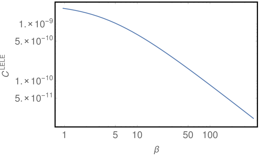
Figure 20: Left panel: Diagram contributing to the matching onto $\bar{L}_{i}E_{j}\,\bar{L}_{k}E_{l}$. The intermediate Higgs propagator is zero-mode subtracted to remove long-distance contributions. Right panel: Wilson coefficient $C^{LELE}_{1111}$ as a function of $\beta$ for $T=1\,{\rm TeV}$, $c_{L_{1}}=-c_{E_{1}}=0.6$ and $Y=\mathds{1}$.

This result can be understood by looking at the defining expression. The scaling with $\beta$ is determined by three factors: the Yukawa matrix scaling, the scaling of the Higgs propagator, and the scaling of the integration variables $x$, $y$ in the relevant integration regions. The two Yukawa couplings each contribute a factor of $\sqrt{\beta}$. The Higgs propagator is slightly more complicated. Let us examine the three terms square brackets in (153) separately. The first term (without step-functions) does not feature an immediate suppression for large $\beta$, since the $1/\beta$ in the prefactor of the square bracket is cancelled. The suppression arises only after integration over the bulk coordinates. To see this, we write $x$ and $y$ in the overall factor $(T^{2}xy)^{\beta}$ as $1/T(1-x_{0}/\beta)$ and $1/T(1-y_{0}/\beta)$, respectively, such that $x_{0}$ and $y_{0}$ measure the distance of $x$, $y$ from the IR brane in units of $1/(\beta T)$, the typical scale for Higgs KK excitations. We then find factors of the form $(1-x_{0}/\beta)^{\beta}$ and $(1-y_{0}/\beta)^{\beta}$, which behave as $e^{-x_{0}}$ and $e^{-y_{0}}$ for large $\beta$, respectively. Hence the first term counts as $\mathcal{O}(1)$ only for $x$ and $y$ within $1/(\beta T)$ of the IR brane. The 5D coordinate integrals then count as $1/(\beta T)$ each, and the contribution of the first term in (153) to the Wilson coefficient is of order $(\sqrt{\beta})^{2}\times 1\times 1/\beta^{2}$, which vanishes for large $\beta$. The remaining two terms in (153) have different properties. There is a global factor of $1/\beta$, but there is no requirement that $x$, $y$ are close to the IR brane. Let us focus on the second term, which is non-zero only for $y>x$. It contains the factor $(x/y)^{\beta}$, which ensures that the contribution to the Wilson coefficient is exponentially suppressed if $x\ll y\,(1-1/\beta)$. Changing integration variables from $x,y$ to $y,x-y$ shows that the integral over $x-y$ counts as $1/(\beta T)$, while the integral over $y$ is effectively unconstrained. Thus the overall total scaling is $(\sqrt{\beta})^{2}\times 1/\beta\times 1/\beta$, which also vanishes for large $\beta$. The same argument with $x\leftrightarrow y$ ensures that the third term in (153) does not contribute to $C^{LELE}_{ijkl}$ for $\beta\to\infty$.

Appendix B KK Higgs contributions

The contribution of KK Higgs modes to $a^{H}_{ij}$ is proportional to the corresponding contribution for the Higgs zero-mode for each diagram topology. It is therefore convenient to study the ratio of the two contributions,

$$R=\frac{a^{H}_{\rm KK}}{a^{H}_{\text{ZM}}}\,.$$ (154)

Up to small corrections this ratio is also independent of the flavour of the propagating states. The Higgs KK contribution can then be obtained by multiplying the zero-mode result by the corresponding $R$. It should be noted that not all topologies shown below actually contribute to $a^{H}_{ij}$ in a specific RS model, either because the combination of SU(2) and U(1) group factors vanishes or because the model does not have Feynman rules that allow for the particular diagram to exist. Note that we do not separate contributions from wrong- and correct-chirality Higgs couplings. The numbers refer to the sum of both type of contributions, and are given by:

$$\includegraphics[width=71.13188pt]{./KKHiggsEx1}R\approx 0.27(0.01) \includegraphics[width=71.13188pt]{./KKHiggsEx2}R\approx 0.27(0.01)$$

$$\includegraphics[width=71.13188pt]{./KKHiggsEx3}R\approx 0.08(0.01) \includegraphics[width=71.13188pt]{./KKHiggsEx4}R\approx 0.08(0.01)$$

$$\includegraphics[width=71.13188pt]{./KKHiggsIntSingle}R\approx 0.15(0.05)$$

$$\includegraphics[width=156.49014pt]{./KKHiggsIntDouble}R\approx 0.77(0.08)$$ (155)

Our error estimates are shown in parenthesis. It arises from the numerical integration error and an estimate for the extrapolation error to $\beta=\infty$, since a numerically stable evaluation is possible only up to $\beta\approx 200-300$. The numerically most challenging diagrams are the ones where the photon is emitted from the Higgs, since they contain products of KK Higgs propagators. We also note that the KK Higgs contribution converges relatively slowly as $\beta\to\infty$, if the diagrams involve an external Higgs attachment to a fermion line in the loop, as illustrated in Figure 21. The typical scaling with powers of $\beta$ in the different momentum regions discussed in the main text does not set in until $\beta\sim 40$. This behaviour agrees with observations made in [20].

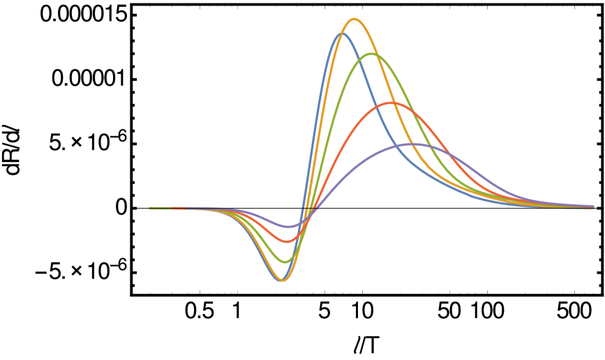
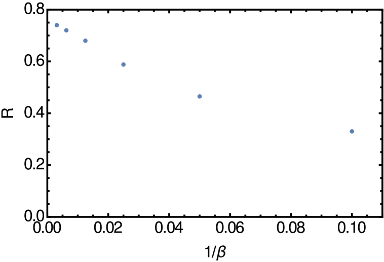
Figure 21: Left panel: $dR/dl$ as a function of the loop momentum for $\beta=$ 10, 20, 40, 80, 160 (curves from left to right) for the diagrams in the last line of (B). Right panel: Corresponding ratio $R$ as a function of $1/\beta$ (no uncertainties shown).

References

- [1] L. Randall and R. Sundrum, Phys. Rev. Lett. 83 (1999) 4690 [hep-th/9906064].
- [2] L. Randall, R. Sundrum, Phys. Rev. Lett. 83 (1999) 3370 [hep-ph/9905221].
- [3] Y. Grossman, M. Neubert, Phys. Lett. B474 (2000) 361 [hep-ph/9912408].
- [4] T. Gherghetta and A. Pomarol, Nucl. Phys. B 586 (2000) 141 [hep-ph/0003129].
- [5] S. J. Huber and Q. Shafi, Phys. Lett. B 498 (2001) 256 [hep-ph/0010195].
- [6] S. J. Huber, Nucl. Phys. B 666 (2003) 269 [hep-ph/0303183].
- [7] K. Agashe, G. Perez and A. Soni, Phys. Rev. D 71 (2005) 016002 [hep-ph/0408134].
- [8] C. Csaki, A. Falkowski and A. Weiler, JHEP 0809 (2008) 008, arXiv:0804.1954 [hep-ph].
- [9] M. Blanke, A. J. Buras, B. Duling, S. Gori and A. Weiler, JHEP 0903 (2009) 001, arXiv:0809.1073 [hep-ph].
- [10] M. Bauer, R. Malm and M. Neubert, Phys. Rev. Lett. 108 (2012) 081603, arXiv:1110.0471 [hep-ph].
- [11] R. Kitano, Phys. Lett. B 481 (2000) 39 [hep-ph/0002279].
- [12] G. Moreau and J. I. Silva-Marcos, JHEP 0603 (2006) 090 [hep-ph/0602155].
- [13] K. Agashe, A. E. Blechman and F. Petriello, Phys. Rev. D 74 (2006) 053011 [hep-ph/0606021].
- [14] C. Csaki, Y. Grossman, P. Tanedo and Y. Tsai, Phys. Rev. D 83 (2011) 073002, arXiv:1004.2037 [hep-ph].
- [15] M. Beneke, P. Dey and J. Rohrwild, JHEP 1308 (2013) 010, arXiv:1209.5897 [hep-ph].
- [16] M. Beneke, P. Moch and J. Rohrwild, Int. J. Mod. Phys. A 29 (2014) 1444011, arXiv:1404.7157 [hep-ph].
- [17] P. Moch and J. Rohrwild, J. Phys. G 41 (2014) 105005, arXiv:1405.5385 [hep-ph].
- [18] W. Buchmüller and D. Wyler, Nucl. Phys. B 268 (1986) 621.
- [19] B. Grzadkowski, M. Iskrzynski, M. Misiak and J. Rosiek, JHEP 1010 (2010) 085, arXiv:1008.4884 [hep-ph].
- [20] K. Agashe, A. Azatov, Y. Cui, L. Randall and M. Son, JHEP 1506 (2015) 196, arXiv:1412.6468 [hep-ph].
- [21] M. C. Chen and H. B. Yu, Phys. Lett. B 672 (2009) 253, arXiv:0804.2503 [hep-ph].
- [22] G. Perez and L. Randall, JHEP 0901 (2009) 077, arXiv:0805.4652 [hep-ph].
- [23] C. Csaki, C. Delaunay, C. Grojean and Y. Grossman, JHEP 0810 (2008) 055, arXiv:0806.0356 [hep-ph].
- [24] K. Agashe, T. Okui and R. Sundrum, Phys. Rev. Lett. 102 (2009) 101801, arXiv:0810.1277 [hep-ph].
- [25] M. Atkins and S. J. Huber, Phys. Rev. D 82 (2010) 056007, arXiv:1002.5044 [hep-ph].
- [26] Y. Kuno and Y. Okada, Rev. Mod. Phys. 73 (2001) 151 [hep-ph/9909265].
- [27] W. -F. Chang and J. N. Ng, Phys. Rev. D 71 (2005) 053003 [hep-ph/0501161].
- [28] K. Agashe, A. Delgado, M. J. May and R. Sundrum, JHEP 0308 (2003) 050 [hep-ph/0308036].
- [29] K. Agashe, R. Contino, L. Da Rold and A. Pomarol, Phys. Lett. B 641 (2006) 62 [hep-ph/0605341].
- [30] M. Carena, S. Casagrande, F. Goertz, U. Haisch and M. Neubert, JHEP 1208 (2012) 156, arXiv:1204.0008 [hep-ph].
- [31] R. Malm, M. Neubert, K. Novotny and C. Schmell, JHEP 1401 (2014) 173, arXiv:1303.5702 [hep-ph].
- [32] A. Azatov, M. Toharia and L. Zhu, Phys. Rev. D 80 (2009) 035016, arXiv:0906.1990 [hep-ph].
- [33] A. Crivellin, S. Najjari and J. Rosiek, JHEP 1404 (2014) 167, arXiv:1312.0634 [hep-ph].
- [34] G. M. Pruna and A. Signer, JHEP 1410 (2014) 14, arXiv:1408.3565 [hep-ph].
- [35] R. Kitano, M. Koike and Y. Okada, Phys. Rev. D 66 (2002) 096002 Erratum-ibid. D 76 (2007) 059902], [hep-ph/0203110].
- [36] A. Crivellin, M. Hoferichter and M. Procura, Phys. Rev. D 89 (2014) 054021, arXiv:1312.4951 [hep-ph].
- [37] A. Crivellin, M. Hoferichter and M. Procura, Phys. Rev. D 89 (2014) 093024, arXiv:1404.7134 [hep-ph].
- [38] M. A. Shifman, A. I. Vainshtein and V. I. Zakharov, Phys. Lett. B 78 (1978) 443.
- [39] A. Azatov, M. Toharia and L. Zhu, Phys. Rev. D 82, 056004 (2010), arXiv:1006.5939 [hep-ph].
- [40] P. R. Archer, M. Carena, A. Carmona and M. Neubert, JHEP 1501 (2015) 060, arXiv:1408.5406 [hep-ph].
- [41] S. M. Barr and A. Zee, Phys. Rev. Lett. 65 (1990) 21 [Erratum-ibid. 65 (1990) 2920].
- [42] D. Chang, W. S. Hou and W. Y. Keung, Phys. Rev. D 48 (1993) 217 [hep-ph/9302267].
- [43] R. G. Leigh, S. Paban and R. M. Xu, Nucl. Phys. B 352 (1991) 45.
- [44] E. E. Jenkins, A. V. Manohar and M. Trott, JHEP 1310 (2013) 087, arXiv:1308.2627 [hep-ph].
- [45] E. E. Jenkins, A. V. Manohar and M. Trott, JHEP 1401 (2014) 035, arXiv:1310.4838 [hep-ph].
- [46] R. Alonso, E. E. Jenkins, A. V. Manohar and M. Trott, JHEP 1404 (2014) 159, arXiv:1312.2014 [hep-ph].
- [47] G. Cacciapaglia, C. Csaki, G. Marandella and J. Terning, JHEP 0702 (2007) 036 [hep-ph/0611358].
- [48] H. Davoudiasl, B. Lillie and T. G. Rizzo, JHEP 0608 (2006) 042 [hep-ph/0508279].
- [49] S. Casagrande, F. Goertz, U. Haisch, M. Neubert and T. Pfoh, JHEP 0810 (2008) 094, arXiv:0807.4937 [hep-ph].
- [50] C. Delaunay, J. F. Kamenik, G. Perez and L. Randall, JHEP 1301 (2013) 027, arXiv:1207.0474 [hep-ph].
- [51] DLMF NIST Digital Library of Mathematical Functions. http://dlmf.nist.gov/, Release 1.0.9 of 2014-08-29.
- [52] F. W. J. Olver and D. W. Lozier and R. F. Boisvert and C. W. Clark, editors. NIST Handbook of Mathematical Functions. Cambridge University Press, New York, NY, 2010.
- [53] S. Weinberg, Phys. Rev. Lett. 19 (1967) 1264.
- [54] U. Bellgardt et al. [SINDRUM Collaboration], Nucl. Phys. B 299 (1988) 1.
- [55] W. H. Bertl et al. [SINDRUM II Collaboration], Eur. Phys. J. C 47 (2006) 337.
- [56] J. Adam et al. [MEG Collaboration], Phys. Rev. Lett. 110 (2013) 201801, arXiv:1303.0754 [hep-ex].
- [57] S. Ahmad, G. Azuelos, M. Blecher, D. A. Bryman, R. A. Burnham, E. T. H. Clifford, P. Depommier and M. S. Dixit et al., Phys. Rev. D 38, 2102 (1988).
- [58] C. Dohmen et al. [SINDRUM II. Collaboration], Phys. Lett. B 317 (1993) 631.
- [59] W. Honecker et al. [SINDRUM II Collaboration], Phys. Rev. Lett. 76 (1996) 200.
- [60] K. A. Olive et al. [Particle Data Group Collaboration], Chin. Phys. C 38 (2014) 090001.
- [61] T. A. Filippas, P. Pabit, R. T. Siegel, and R. E. Welsh, Phys. Lett. 6, 118 (1963)
- [62] T. Suzuki, D. F. Measday and J. P. Roalsvig, Phys. Rev. C 35 (1987) 2212.
- [63] J. Baron et al. [ACME Collaboration], Science 343 (2014) 269, arXiv:1310.7534 [physics.atom-ph].
- [64] B. Aubert et al. [BaBar Collaboration], Phys. Rev. Lett. 104 (2010) 021802, arXiv:0908.2381 [hep-ex].
- [65] K. Hayasaka et al. [Belle Collaboration], Phys. Lett. B 666, 16 (2008), arXiv:0705.0650 [hep-ex].
- [66] R. Aaij et al. [LHCb Collaboration], Phys. Lett. B 724 (2013) 36, arXiv:1304.4518 [hep-ex].
- [67] M. Aoki [DeeMe Collaboration], AIP Conf. Proc. 1441 (2012) 599.
- [68] R. M. Carey et al. [Mu2e Collaboration], FERMILAB-PROPOSAL-0973.
- [69] Y. G. Cui et al. [COMET Collaboration], KEK-2009-10.
- [70] A. M. Baldini, F. Cei, C. Cerri, S. Dussoni, L. Galli, M. Grassi, D. Nicolo and F. Raffaelli et al., arXiv:1301.7225 [physics.ins-det].
- [71] N. Berger [Mu3e Collaboration], Nucl. Phys. Proc. Suppl. 248-250 (2014) 35.
- [72] J. A. Cabrer, G. von Gersdorff and M. Quiros, Phys. Rev. D 84 (2011) 035024, arXiv:1104.3149 [hep-ph].
- [73] P. Moch and J. Rohrwild, Nucl. Phys. B 902 (2016) 142, arXiv:1509.04643 [hep-ph].
- [74] J. A. M. Vermaseren, Comput. Phys. Commun. 83 (1994) 45.
- [75] D. Binosi and L. Theussl, Comput. Phys. Commun. 161 (2004) 76 [hep-ph/0309015].