The star formation rate cookbook at $1<z<3$:
Extinction-corrected relations for UV $\&$ [OII]$\lambda$3727 luminosities

Abstract

Aims. In this paper we use a well-controlled spectroscopic sample of galaxies at $1{<}z{<}3$ drawn from the Galaxy Mass Assembly ultra-deep Spectroscopic Survey (GMASS) to study different star formation rate (SFR) estimators. In particular, we use infrared (IR) data to derive empirical calibrations to correct ultraviolet (UV) and [OII]$\lambda$3727 luminosities for dust extinction and dust-corrected estimates of SFR.

Methods. We selected 286 star-forming galaxies with spectroscopic redshift $1{<}z{<}3$. In order to have a homogeneous wavelength coverage in the spectra, the sample was divided into two sub-groups: galaxies at $1{<}z{<}1.6$ whose spectra cover the rest-frame range ${\sim}2700{-}4300\AA$, where the [OII]$\lambda$3727 emission line can be observed, and galaxies at $1.6{<}z{<}3$ whose spectra cover the range ${\sim}1100{-}2800\AA$. In the selection procedure we fully exploit the available spectroscopic information. In particular, on the basis of three continuum indices, we are able to identify and exclude from the sample galaxies in which old stellar populations might bring a non-negligible contribution to IR luminosity ($L_{IR}$) and continuum reddening. Using Spitzer-MIPS and Herschel-PACS data we derive $L_{IR}$ for two-thirds of our sample. The $L_{IR}/L_{UV}$ ratio is used as a probe of effective attenuation ($A_{IRX}$) to search for correlations with continuum and spectroscopic features in order to derive empirical calibrations to correct UV and [OII]$\lambda$3727 luminosities for dust extinction.

Results. Through the analyses of the correlations between different dust attenuation probes, a set of relations is provided that allows the recovery of the total unattenuated SFR for star-forming galaxies at $1{<}z{<}3$ using UV and [OII]$\lambda$3727 luminosities.

The relation between $A_{IRX}$ and UV continuum slope ($\beta$) was tested for our sample and found to be broadly consistent with the literature results at the same redshift, though with a larger dispersion with respect to UV-selected samples.

We find a correlation between the rest-frame equivalent width of the [OII]$\lambda 3727$ line and $\beta$, which is the main result of this work. We therefore propose the rest-frame equivalent width of the [OII]$\lambda 3727$ line as a dust attenuation probe and calibrate it through $A_{IRX}$, though the assumption of a reddening curve is still needed to derive the actual attenuation towards the [OII]$\lambda 3727$ line ($A_{[OII]}$). We tested the issue of differential attenuation towards stellar continuum and nebular emission: our results are in line with the traditional prescription of extra attenuation towards nebular lines.

Finally, we use our set of cross-calibrated SFR estimates to look at the relation between SFR and stellar mass. The galaxies in our sample show a close linear relation ($\sigma{=}0.3$ dex) at all redshifts with a slope ${\sim}0.7-0.8$, which confirms several previous results.

1 Introduction

In the past decades, great effort has been devoted to the study of the Universe in the redshift range $1{<}z{<}3$. Several studies have shown that this is the epoch when a substantial fraction of galaxy mass assembly took place, and when there is a peak in the evolution of the star formation rate (SFR) density through cosmic time (Lilly et al. 1996; Madau et al. 1996; Dickinson et al. 2003; Hopkins & Beacom 2006; Daddi et al. 2007). In this epoch a critical transformation phase is believed to have occurred, revealed by the observed changes in the colour-mass plane where a significant fraction of galaxies moves from the blue cloud of active star formation to the red sequence inhabited by spheroidal galaxies with weak or suppressed star formation at $z{<}1$ (e.g. Cassata et al. 2008; Cimatti et al. 2013).

A key element in the study of galaxy evolution is obviously the availability of large samples of galaxies. Spectroscopic redshift surveys play a crucial role as they provide samples with confirmed redshifts. Though photometric redshift surveys have now reached a high level of accuracy, the number of catastrophic failures, even if low at a few percent (Ilbert et al. 2013), could still produce large unknowns. Moreover, spectroscopy provides information that is not accessible by broad-band photometry, e.g. emission line fluxes and absorption features that are fundamental to gaining insight on gas properties and therefore dust extinction, star formation, and feedback mechanisms.

Astronomical observation plans are actually going in the direction of collecting spectroscopic information for increasingly large samples of galaxies, as confirmed by the number of spectroscopic surveys that have been carried out in recent years or are planned for the near future (e.g. K20 (Mignoli et al. 2005), VVDS (Le Fèvre et al. 2005), Deep2 (Willmer et al. 2006), zCOSMOS (Lilly et al. 2007), ESO-GOODS (Vanzella et al. 2008; Popesso et al. 2009; Balestra et al. 2010), PRIMUS (Coil et al. 2011), GMASS (Kurk et al. 2013), DEIMOS/Keck (Kartaltepe et al., in prep.; Capak et al., in prep.), VUDS (Le Fèvre et al. 2015), MOSDEF (Kriek et al. 2015), VANDELS, BigBOSS (Schlegel et al. 2011), Euclid (Laureijs et al. 2011), WFIRST (Spergel et al. 2013)). The large number of high-redshift galaxy spectra that is rapidly becoming available inspires the need to test existing analysis methods and calibrations, and to create new ones, to correctly interpret the wealth of spectroscopic information in the frame of understanding the main processes that regulate galaxy evolution.

The rate at which a galaxy produces stars is a critical ingredient to the investigation of galaxy evolution. Though other properties like stellar mass can be quite robustly estimated from SED fitting to photometric data, there is still room for improvement in our ability to estimate the star formation rate (SFR) at high redshift because of the uncertainties in the assumptions made in translating integrated fluxes and colours to an estimate of the SFR (Madau & Dickinson 2014; Pannella et al. 2015).

The rest-frame UV continuum light emitted by young massive stars and the H$\alpha$ optical emission line are very good and primary tracers of star formation (e.g. Kennicutt 1998; Kennicutt & Evans 2012). At high redshift, where H$\alpha$ is less easily accessible, the [OII]$\lambda$3727 emission line can be a fair alternative. However, these primary and secondary tracers are known to be affected by the presence of dust that absorbs the flux emitted at UV and optical wavelengths, and re-emits it at longer wavelengths in the infrared (IR) regime. The use of dust-unbiased tracers like mid- and far-IR (FIR) or radio continuum would be preferable, but it is still limited at high redshift due to sensitivity limits. Giant strides have been made in this respect with the advent of the Spitzer and Herschel telescopes in the last decade (see e.g. Lutz et al. 2011; Rodighiero et al. 2010a; Elbaz et al. 2011; Nordon et al. 2013; Oteo et al. 2014), but the low-SFR regimes at high redshift can still only be accessed by means of stacking (Rodighiero et al. 2014; Pannella et al. 2015). In order to study star-forming galaxies in a large range of SFR, UV and line emission luminosities are still the best choice for cosmologically relevant galaxy samples, and the study of reliable corrections for dust attenuation continues to be a crucial topic.

Dust attenuation affecting emission line luminosities can be derived by measuring the Balmer decrement in galaxy spectra (Brinchmann et al. 2004; Garn et al. 2010), but this information is still rarely available at high redshift. Indirect ways to correct for dust extinction are often employed, such as the comparison with other estimates of SFR like the value derived from SED fitting to broad-band photometry (Förster Schreiber et al. 2009) under the assumption of some attenuation curves (e.g. Calzetti et al. 2000).

The dust correction of UV light commonly relies on the local correlation between the slope of the UV continuum and dust attenuation (Meurer et al. 1999; Calzetti et al. 2000; Daddi et al. 2004; Overzier et al. 2011; Takeuchi et al. 2012), though the general validity of such correlation, especially at high redshift, is still under debate (Calzetti 2001; Boissier et al. 2007; Seibert et al. 2005; Reddy et al. 2010, 2012, 2015; Overzier et al. 2011; Takeuchi et al. 2012; Buat et al. 2012; Heinis et al. 2013; Nordon et al. 2013; Castellano et al. 2014; Oteo et al. 2013, 2014; Hathi et al. 2015).

Though the data coming from recent IR surveys are not sufficient to map the population of SFGs down to low-SFR regimes, they can be effectively used to test the existing calibrations of dust extinction correction recipes, or to derive new ones. This can be made under the assumption that the IR emission depends only on the absorption of the flux emitted by the young stars responsible of UV light. However, there might be a non-negligible contribution of old stars to the dust heating that grows with decreasing sSFR (da Cunha et al. 2008; Kennicutt & Evans 2012; Arnouts et al. 2013; Utomo et al. 2014), leading to an overcorrection of UV light when IR luminosity ($L_{IR}$) is used as dust correction probe. A way to overcome this problem is to use spectroscopic samples, where continuum indices may be computed that indicate the possible presence of old stellar populations (Bruzual A. 1983; Daddi et al. 2005; Cimatti et al. 2008).

In this paper, different indicators of star formation for a sample of $1<z<3$ galaxies will be analysed. We concentrate on a well-controlled spectroscopic sample, rich of ancillary panchromatic photometric data, including IR from Spitzer and Herschel, in order to focus on the information that can be obtained from spectra. We will use the IR-derived SFR as a benchmark against which compare other estimates at shorter wavelengths, namely UV and [OII]$\lambda 3727$ luminosities, and to derive new (or update existing) calibrations of dust extinction correction recipes. This way we are able to build a set of self-consistent recipes to derive the total un-extincted SFR, which are collected in a Table at the end of the paper.

Throughout this paper, we adopt $H_{0}{=}70$ km/s/Mpc, $\Omega_{m}{=}0.3$, $\Omega_{\Lambda}{=}0.7$, give magnitudes in AB photometric system, and assume a Kroupa (2001) initial mass function. All linear fits, unless differently stated in the text, will be ordinary least squares (OLS) regressions of Y on X (Y$|$X) (Bevington 1969; Isobe et al. 1990). Finally, we will indicate with the suffix ”0” all un-extincted quantities, i.e. quantities corrected for dust extinction.

2 The multi-wavelength dataset

The main ingredient of the present study is a well-controlled spectroscopic sample at $1<z<3$ selected from the photometric catalogue of the Galaxy Mass Assembly ultra-deep Spectroscopic Survey (GMASS).

2.1 The GMASS survey

The GMASS survey (Kurk et al. 2013) is an ESO VLT large program project based on data acquired using the FOcal Reducer and low dispersion Spectrograph (FORS2). The project’s main science driver is to use ultra-deep optical spectroscopy to measure the physical properties of galaxies at redshifts $1.5{<}\emph{z}{<}3$. The GMASS photometric catalogue is a pure magnitude limited catalogue from the GOODS-South public image in the IRAC band at $4.5\mu m$: $\emph{m}_{4.5}{<}23.0$ (AB system). In the chosen redshift range this selection is most sensitive to stellar mass. In particular, the limiting mass sensitivities are $log(M/M_{\odot})\sim$ 9.8, 10.1, and 10.5 for $z=$ 1.4, 2, and 3, respectively. The GMASS photometric catalogue gathers information from U band to IRAC 8.0 $\mu$m band of 1277 objects.

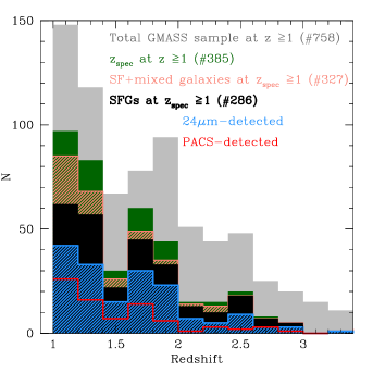
Figure 1: Redshift distribution of total GMASS sample at $z\geq 1$ with either spectroscopic or photometric redshift (grey); GMASS sample at $z_{spec}\geq 1$ with reliable spectroscopic redshift (green); preliminary sample of 327 SF+mixed galaxies (salmon); final sample of 286 SFGs analysed in the paper (black); $24\mu m$-detected SFGs (blue); PACS-detected SFGs (red).

2.2 Spectroscopic data

From the GMASS photometric catalogue, 170 objects were selected as main targets to be observed (250 objects including fillers) during 145h, and a secure spectroscopic redshift could be determined for 131 of them. The spectral resolution of GMASS spectra is $R=\lambda/\Delta\lambda\sim 600$. To extend our analysis, we collected public spectra from other spectroscopic surveys for the galaxies in the GMASS photometric catalogue with no GMASS spectrum. In particular, we searched for counterparts of GMASS galaxies from the following surveys: the ESO-GOODS/FORS2 v3.0 (Vanzella et al. 2008) and ESO-GOODS/VIMOS 2.0 (Popesso et al. 2009; Balestra et al. 2010), the VVDS v1.0 (Le Fèvre et al. 2005), and the K20 (Mignoli et al. 2005). We refer the reader to the cited papers for more information about the various surveys.

A total of 385 galaxies with a reliable spectroscopic redshift $z>1$, coming from any one of the cited spectroscopic surveys, was selected (see Fig. 1).

2.3 Mid- and far-IR photometry

The GOODS-South field has been observed with the Photodetector Array Camera and Spectrometer (PACS; Poglitsch et al. (2010)) on board the Herschel Space Observatory as part of two projects: the PACS Evolutionary Probe (PEP; Lutz et al. (2011)) and the GOODS-Herschel (Elbaz et al. 2011) programmes. The publicly released PACS catalogue produced using as priors the source positions expected on the basis of a deep Spitzer-MIPS 24 $\mu m$ catalogue (Magnelli et al. 2011) was used in this work. We refer the reader to Magnelli et al. (2013) for all the details about data reduction and the construction of images and catalogues. The public catalogue presented in Magnelli et al. (2013) has a 24 $\mu m$ flux cut at 20$\mu Jy$. We extended it to fainter fluxes with a 24 $\mu m$ source catalogue from Daddi et al. (in prep.) that was created, similarly to the Magnelli et al. (2011) one, using a PSF fitting technique at the 3.6 $\mu m$ source positions as priors.

GMASS coordinates of the 385 galaxies at $1{<}z_{spec}{<}3$ were matched to the sources listed in the 24 $\mu m$ source catalogues. Counterparts were searched within an angular separation of 1.4”. After some tests, this angular separation was chosen as the best compromise not to lose real counterparts, while minimizing the selection of false pairs. 236 24 $\mu m$ counterparts were found, 121 of which have at least one PACS detection.

3 Selection of the star-forming galaxies (SFGs)

Since the aim of this work is to study the star formation in star-forming galaxies (SFGs) at $1{<}z{<}3$, the catalogue assembled of 385 galaxies at $z_{spec}{\geq}1$ had to be cleaned of quiescent objects and active galactic nuclei (AGNs).

On the basis of the spectroscopic features, 33 quiescent galaxies were identified and excluded from the sample. Their average spectrum (Fig. 2) shows the characteristic features of the rest-frame UV spectrum of old and passive stellar populations: the very red continuum, characterized by prominent breaks (at 2640$\AA$, 2900$\AA$, 4000$\AA$) and rich of metal absorptions (e.g. CaII H$\&$K doublet) (Cimatti et al. 2008; Mignoli et al. 2005), and the weakness or complete absence of [OII]$\lambda$3727 emission line. We will come back on the shape of the continuum of old stellar populations later in this section.

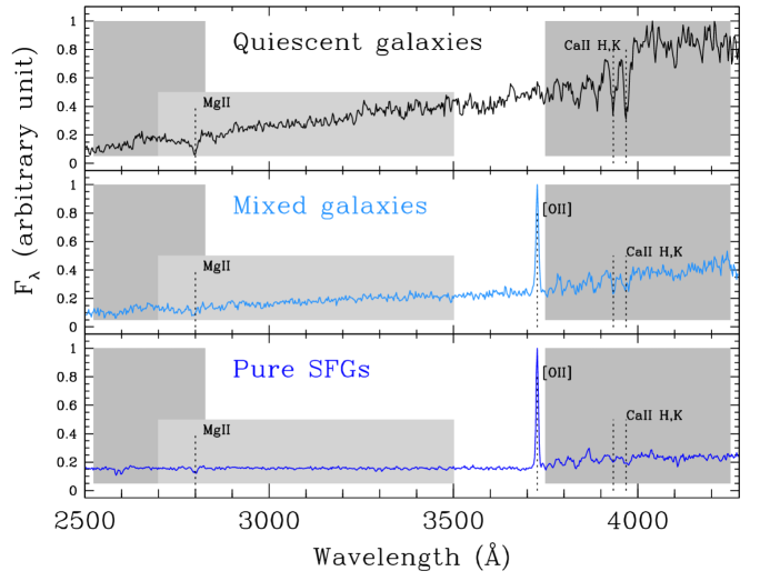
Figure 2: From top to bottom: a) average spectrum of 33 quiescent galaxies in the GMASS sample; b) average spectrum of mixed galaxies in the [OII] sample, at $1{<}z{<}1.6$; c) average spectrum of not-mixed SFGs in the [OII] sample, at $1{<}z{<}1.6$. Mixed galaxies have high values of the three continuum indices indicated by grey shaded regions: MgUV ($2600-2900\AA$) (Daddi et al. 2005); $C(29-33)$ ($2900-3300\AA$) (Cimatti et al. 2008); $D4000$ break ($3750-4250\AA$) (Bruzual A. 1983). See the text and Fig. 4 for more details.

A combination of spectroscopic features and X-ray information was instead used to identify AGN hosts. In particular, we excluded galaxies showing typical broad and/or narrow emission lines (e.g. CIV$\lambda$1549$\AA$, MgII$\lambda$2800). We also excluded galaxies with an X-ray detection from the Chandra 4Ms catalogue (Xue et al. 2011), and absorption-corrected rest-frame 0.5-8 kev luminosity higher than $L_{x}=3x10^{42}$ erg/s, following the criteria for AGN identification given by Xue et al. (2011). This selection made us discard 25 more galaxies from the sample. The objects with an X-ray detection, but $L_{x}<3x10^{42}$ erg/s were instead kept in the sample.

The remaining, at this stage, 327 galaxies showed spectroscopic features typical of SFGs and lack of AGN evidence from the X-rays. UV spectroscopic features identifying a SFG are the presence of strong nebular emission lines, such as [OII]$\lambda$3727, and/or a blue UV continuum. Not all the features can be detected in all the spectra because, given the wide range of redshifts covered by our sample, the galaxy spectra sample different rest-frame wavelength ranges. In particular, we can roughly divide the sample into two sub-groups: galaxies at $1{<}z{<}1.6$ that cover the range $\sim 2700-4300\AA$ ([OII] sample), where the [OII]$\lambda$3727 emission line can be observed; and galaxies at $1.6{<}z{<}3$ that cover the range $\sim 1100-2800\AA$ (UV sample), in whose spectra strong inter-stellar medium (ISM) absorption lines can be detected (see Fig. 3).

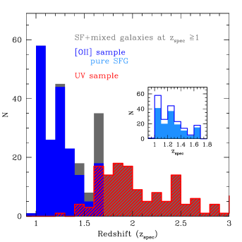
Figure 3: Redsfhit distribution. Big plot: the grey histogram represents the preliminary selection of 327 SF+mixed galaxies; the blue histogram represents the [OII] sample (i.e. spectra covering the wavelength range $\sim 2700-4300\AA$); the red histogram represents the UV sample (i.e. spectra covering the wavelength range $\sim 1100-2800\AA$). Little inset: zoom of the [OII] sample: empty blue histogram represents the total [OII] sample, while light blue shaded histogram represents only not-mixed SFGs in the [OII] sample.

3.1 Spotting the presence of old stellar populations in SFGs

In this work we decided to use $L_{IR}$ as benchmark SFR indicator, exploiting the recent HERSCHEL data in combination with deep spectroscopy. $L_{IR}$ is the bolometric luminosity coming from dust emission and can be directly converted into the rate of obscured star formation (Kennicutt 1998; Kennicutt & Evans 2012). The validity of such conversion relies on the assumption that only young star populations (the ones responsible for the UV luminosity emission) heat the dust that than re-emits in the IR. However, there might be a non-negligible contribution of old stars to the dust heating that grows with decreasing sSFR (da Cunha et al. 2008; Kennicutt & Evans 2012; Arnouts et al. 2013; Utomo et al. 2014), leading to an overestimate of the true SFR when using $L_{IR}$ as sole estimator.

Thanks to the spectroscopic information we are able to overcome this issue. In the wavelength range covered by our spectra three continuum indices may be computed that indicate the possible presence of old stellar populations. These indices are: MgUV, which is a feature produced by the combination of the strongest breaks and absorptions at $2600-2900\AA$ (Daddi et al. 2005); $C(29-33)$, which is a colour index of the UV continuum defined at $2900-3300\AA$ (Cimatti et al. 2008); and the $D4000$ break (Bruzual A. 1983). We refer the reader to the cited papers for the definitions of the indices. The range over which each parameter is defined is indicated in Fig. 2.

Typically, early-type galaxies have $MgUV>1.2$, $C(29-33)>0.6$, $D4000>1.6$ (Daddi et al. 2005; Cimatti et al. 2008; Mignoli et al. 2005; Kauffmann et al. 2003; Hathi et al. 2009). We measured the indices on the spectra of the 327 galaxies resulting from the previous selection in order to search for evidence of the possible presence of old stellar populations along the young ones.

[OII] sample

Given the different rest-frame wavelength coverage of the spectra, not all indices are available for all galaxies. The spectra of the galaxies in the [OII] sample always have at least one index (often two) in their range. We find that $22\%$ of the [OII] sample have a continuum suggesting the presence of an old stellar population that might contribute to dust heating and to the reddening of the UV continuum. The parameters distributions are shown in Fig. 4, and the mean value of each index measured on the 33 quiescent galaxies is also indicated as reference. To make a distinction, we will call the objects whose indices are above the threshold mixed galaxies (because they show both the [OII]$\lambda$3727 line and a red continuum), while the objects whose indices are below the thresholds will be referred to simply as SFGs in the rest of the paper. The relative redshift distributions of the two classes are shown in Fig. 3. The average spectrum of mixed galaxies, presented in Fig. 2, though showing the [OII]$\leavevmode\nobreak\ \lambda 3727$ emission line, has a continuum shape more similar to that of quiescent galaxies, whose average spectrum is shown as reference. Only SFGs (i.e. not-mixed) are used in our analysis.

UV sample

In the UV sample only the MgUV index is available in the spectrum of $\sim 45\%$ of the sample. For the remaining $\sim 55\%$ of the UV sample no index is available. When in range, the MgUV index is always $<1.2$, within the errors. Moreover, all the galaxies in the UV sample (with and without measurable MgUV index) have the bluest colour in the (NUV-r) vs. (r-K) colour-colour plot, implying that they have the highest sSFR (Arnouts et al. 2013). This means that in these galaxies a possible contribution of old stellar populations to dust heating should be negligible (see also Utomo et al. 2014). Therefore we classify all the galaxies in the UV sample as not-mixed SFGs, and include them all in the analysis.

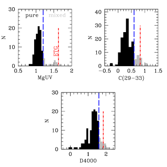
Figure 4: Continuum indices distribution over the [OII] sample: MgUV, C(29-33), D4000. In each plot the blue vertical line represents the threshold that separates SFGs from mixed galaxies (see the text for more details). The red lines mark the average value of each index measured on the GMASS quiescent galaxies at $z_{spec}\geq 1$, for reference.

3.2 Summary of the final sample selection

Table 1: Summary table of the general properties (spectral classes, X-ray and IR detections) of the GMASS spectroscopic sample at $z_{spec}\geq 1$.

GMASS galaxies with spectroscopic data and reliable spectroscopic redshift ($z_{spec}\geq 1$)
[OII] sample 219 objs.		quiescent	SFG	AGN	$L_{X}{>}3{\times}10^{42}$erg/s	$L_{X}{<}3{\times}10^{42}$erg/s	NO $L_{X}$	$24\mu$ m	PACS
	quiescent	21	0	0	0	4	17	6	4
Spectral	SFG		192	0	4	15	173	130	72
class	AGN			6	2	0	4	3	1
	$L_{X}{>}3{\times}10^{42}erg/s$				6	0	0	6	3
X-ray	$L_{X}{<}3{\times}10^{42}erg/s$					19	0	15	11
	NO $L_{X}$						194	118	63
IR	$24\mu$ m							139	77
data	PACS								77
UV sample 166 objs.		quiescent	SFG	AGN	$L_{X}{>}3{\times}10^{42}$erg/s	$L_{X}{<}3{\times}10^{42}$erg/s	NO $L_{X}$	$24\mu$ m	PACS
	quiescent	12	0	0	1	1	10	4	3
Spectral	SFG		148	0	9	3	136	88	36
class	AGN			6	5	0	1	5	5
	$L_{X}{>}3{\times}10^{42}$erg/s				15	0	0	12	10
X-ray	$L_{X}{<}3{\times}10^{42}$erg/s					4	0	2	1
	NO $L_{X}$						147	83	33
IR	$24\mu$ m							97	44
data	PACS								44

Table 2: Summary table of the general properties (spectral classification and continuum indices, X-ray, and IR detections) of SFGs and mixed galaxies (Tot. 327 galaxies).

	z	Spec.	$L_{X}$	Tot.	MgUV	C(29-33)	D4000	no IR	MIPS		PACS
		class	(erg/s)	num.					$24\mu$ m	$70\mu$ m	$100\mu$ m	$160\mu$ m
UV sample	$1.6{-}3.0$	pure SFG	${<}3{\times}10^{42}$	3	$1.07$	${-}$	${-}$	1	2	0	0	1
		pure SFG	NO	136				58	78	4	25	19
[OII] sample	$1.0{-}1.6$	pure SFG	${<}3{\times}10^{42}$	9	$1.06$	$0.31$	$1.30$	0	9	2	6	5
		pure SFG	NO	138				50	88	11	42	37
		mixed	${<}3{\times}10^{42}$	6	$1.49$	$0.74$	$1.80$	2	4	2	4	4
		mixed	NO	35				10	25	2	12	9

From the magnitude limited GMASS photometric catalogue we preliminary selected 327 galaxies with a secure spectroscopic redshift $1{<}z{<}3$, typical spectroscopic features associated to star formation (presence of [OII]$\lambda$3727 emission line and/or a blue continuum), and lack of evidence of AGN presence from the X-rays. We summarize the main properties of the parent spectroscopic sample in Table 1, and give additional information on the preliminary sample of 327 galaxies in Table 2. A deeper spectroscopic analysis of the preliminary selection of galaxies revealed the possible presence of old stellar populations in $\sim 12\%$ of them. These 41 mixed galaxies will be excluded from the analysis because of the possible contribution of old stars to dust heating and continuum reddening. The 286 SFGs will be used to study the relations between different estimators of SFR. In the rest of the paper, when talking about SFGs we will refer to the not-mixed ones. In Table 3 we report some additional spectroscopic information about the 286 SFGs.

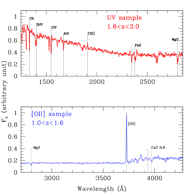
Figure 5: Top: average spectrum of SFGs in the UV sample, at $1.6{<}z{<}3$; bottom: average spectrum of SFGs in the [OII] sample, at $1{<}z{<}1.6$.

On the basis of the wavelength coverage of the spectra, the sample can be roughly divided into two sub-groups: galaxies at $1{<}z{<}1.6$ whose spectra cover the range $\sim 2700-4300\AA$, and galaxies at $1.6{<}z{<}3$ whose spectra cover the range $\sim 1100-2800\AA$. We will refer to these groups, respectively, as the [OII] sample and the UV sample. In Fig. 5 the average spectra of the galaxies of the two sub-samples are shown.

3.3 Comparison to the parent sample

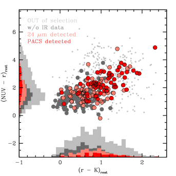
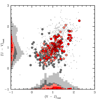
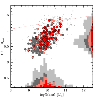
Figure 6: From top-left, clockwise: a) rest-frame (NUV-r)vs.(r-K) colour diagram (Arnouts et al. 2013); b) rest-frame (U-V)vs.(V-J) colour diagram (Williams et al. 2009); c) rest-frame colour (U-B) vs. stellar mass diagram. The red dotted line is the red sequence at $z\sim 2$ defined in Cassata et al. (2008). In all plots, small light grey dots represent the GMASS parent sample at $z{\geq}1$, while large points represent the final sample of 286 SFGs analysed in the paper. In particular: dark grey points indicate galaxies without IR data; salmon points indicate galaxies with a 24$\mu m$ detection; red points indicate galaxies with at least one PACS detection. The distribution of each quantity is shown by light grey histograms for the GMASS parent sample ($\#758$), while dark grey histograms represent the distribution over the SFGs sample; salmon histograms represent galaxies with a 24$\mu m$ detection; red histograms represent galaxies with at least one PACS detection.

It is important to establish which part of the galaxy population at $1{<}z{<}3$ is represented by our sample. The main bias of our sample comes from two elements: the requirement of a spectroscopic redshift, and the different detection limits of the various sets of photometric data, in particular the IR ones from Spitzer and Herschel. To place our galaxies into context, we compared their distributions of mass and colours to those of the full GMASS sample in the same redshift range (Fig. 6). Here we note that GMASS is basically a mass-selected sample, whose limiting mass sensitivity over the entire redshift range of our choice ($1{<}z{<}3$) is $log(M/M_{\odot}){\sim}10.5$ (Kurk et al. 2013).

Compared to the reference sample, the SFGs sample is probing intermediate-mass objects, the median mass being $M_{\star}{=}10^{9.8}M_{\odot}$, therefore our sample is not mass-complete. The sample is biased towards bluer and less massive objects, as can be seen from the colour-mass diagram (Fig. 6 c)), with the reddest and more massive tail populated mainly by the IR-detected galaxies. Objects in the red sequence may be either quiescent/passive galaxies or dusty SFGs. The degeneracy can be broken by using colour-colour diagrams (Fig. 6 a), b)). The position of our selection of SFGs in the (NUV-r)vs.(r-K) and the (U-V)vs.(V-J) diagrams indicates that we have selected galaxies with the highest sSFR, with respect to the parent sample (Williams et al. 2009; Arnouts et al. 2013), of which the IR-detected are the dustier ones.

The different detection limits of the used datasets translate into lower limits in the SFRs that can be probed by a specific indicator. In particular, UV- and optical-based SFR estimators are the deepest ones and allow values down to a few $M_{\odot}yr^{-1}$ to be reached at $z{\sim}1$. Mid-IR data have slightly higher SFR thresholds, while far-IR data are available only for the most star-forming galaxies: $\sim 100M_{\odot}yr^{-1}$ at $z{\sim}2$ and $\sim 10M_{\odot}yr^{-1}$ at $z{\sim}1$ (Elbaz et al. 2011; Rodighiero et al. 2011).

In the regime of star formation probed by mid- and far-IR data we will derive new relations to correct UV- and optical-based estimators for dust extinction. Then, we will test the robustness of extending such calibrations in lower star formation regimes by comparing one another the newly calibrated estimators for galaxies without IR data.

Though our sample is inevitably not complete, Fig. 6 shows that it is fairly representative of a specific galaxy population whose properties may be summarized as follows:

• redshift between $z\sim 1$ and $z\sim 3$;

• intermediate stellar mass (approximately in the range $10^{9.2}{<}M/M_{\odot}{<}10^{10.2}$);

• blue rest-frame colours: $(NUV-r){<}3\ \&\ (r-K){<}1.4$ or
  $(U-V){<}1.2\ \&\ (V-J){<}1.5$.

All the relations derived in the paper should be used within these boundaries. We also note that the use of our relations is not recommended for galaxies whose spectral continuum indices show strong evidence of old stellar populations ($MgUV{>}1.2$, $C(29-33){>}0.6$, $D4000{>}1.6$) because they could cause an over-correction of dust extinction of either UV or [OII]$\lambda$3727 luminosity and consequently an over-estimate of the total SFR of the galaxy.

Table 3: Number of spectra collected from the different surveys, for the final selection of 286 SFGs. The observed spectral resolution ($R=\lambda/\Delta\lambda$) for each survey is also indicated.

	GMASS	ESOFORS	ESOVIMOS	VVDS	K20
R	600	660	180,580	230	260,380,660
N.	131	78	38	9	30

4 The benchmark: SFR based on IR luminosity

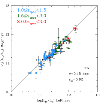
Figure 7: $L_{IR}$ computed using UV to far-IR photometry and the MAGPHYS code vs. $L_{IR}$ computed using Mid- to far-IR photometry and the LePhare code. Points are colour-coded with respect to their redshift. Correlation coefficient $r_{xy}$ (logarithmic scale) is also indicated.

The total infrared luminosity ($L_{IR}$) is defined as the integrated luminosity between 8-1000 $\mu m$. To derive $L_{IR}$ for the sources with at least two IR photometric points (i.e. 24 $\mu m$ plus at least one Herschel band), we performed an SED fitting procedure, based on $\chi^{2}$ minimization, using the MAGPHYS code in its default configuration (da Cunha et al. 2008) and all the available photometric information, from U band to PACS data. The inclusion of the whole SED in the fitting procedure allowed us to fully exploit the photometric information. Following an established procedure (Rodighiero et al. 2010a, b; Gruppioni et al. 2010; Cava et al. 2010; Popesso et al. 2012), we anchored the spectral fit to the FIR Spitzer-Herschel data-points by increasing the photometric errors of the bands from U to 8$\mu$m (up to 10$\%$). For each source, the 50th percentile of the $L_{IR}$ distribution was taken as the best-value; the quoted uncertainty is the 68th percentile range (${\sim}1{\sigma}$).

To assess the robustness of the resulting quantity, $L_{IR}$ was also computed by fitting the mid- to far-IR photometry alone to a compilation of IR SED template libraries (Chary & Elbaz 2001; Dale & Helou 2002; Lagache et al. 2004; Rieke et al. 2009) using the LePhare code (Arnouts et al. 1999; Ilbert et al. 2006). The two estimates were found to be highly consistent (see Fig. 7). This test was in line with the results by Berta et al. (2013) who demonstrated that the different methods commonly used in the literature to recover $L_{IR}$ all give consistent estimates when Herschel photometry is implemented in SED fitting.

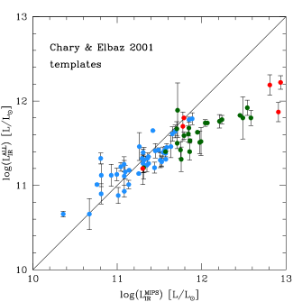
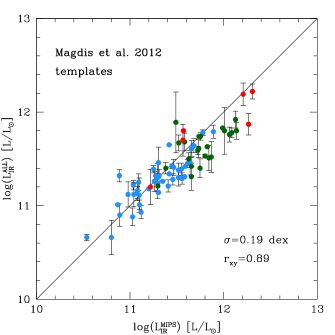
Figure 8: Comparison between $L_{IR}$ computed with MAGPHYS using all the available photometric bands (from U-band to PACS), and $L_{IR}$ computed using only the 24 $\mu m$ band and, respectively, Chary & Elbaz (2001) templates (top) and Magdis et al. (2012) templates (bottom). Points are colour-coded with respect to their redshift (see Fig. 7 for the legenda).

To improve the statistics of the sample, especially at low luminosities, $L_{IR}$ was computed also for those galaxies with a detection at 24 $\mu m$ but no PACS data. At high redshift ($z{\sim}2$), locally calibrated IR templates have difficulties in recovering bolometric $L_{IR}$ of highly luminous galaxies from the 24 $\mu m$ flux alone (Elbaz et al. 2011; Nordon et al. 2010). Several methods have been proposed to re-calibrate the 24 $\mu m$ flux density (Murphy et al. 2011; Elbaz et al. 2011; Nordon et al. 2013) that make use of the traditional IR templates whose resulting $L_{IR}$ values need to be corrected using various prescriptions. The majority of these conversions from 24 $\mu m$ to $L_{IR}$ either produce trends and biases with the ”true” $L_{IR}$ (defined as the one derived from HERSCHEL data), or include non-linear scaling that strongly increase the scatter (Nordon et al. 2013).

A different approach is to build brand new SED templates taking advantage of the most recent far-IR and sub-mm data. This latter method is preferable since it does not need to apply a posteriori corrections to the resulting $L_{IR}$ values. Here we adopted the main sequence templates of Magdis et al. (2012) to extrapolate $L_{IR}$ from the 24 $\mu m$ flux densities. We tested this choice for the sub-sample of PACS-detected galaxies trough the comparison between $L_{IR}$ derived from 24 $\mu m$ alone and $L_{IR}$ computed using all available photometric data from U-band to PACS, as explained in the previous paragraph. The result of this test is shown in Fig. 8 where we also show, for comparison, the output of using the popular Chary & Elbaz (2001) templates. The Chary & Elbaz (2001) templates work well up to $z{\sim}1$, but at higher redshifts they overestimate the true $L_{IR}$, mainly because at such redshifts polycyclic aromatic hydrocarbon (PAH) emissions contribute significantly to the 24 $\mu m$ band flux and are difficult to model (Elbaz et al. 2011; Nordon et al. 2010). With the Magdis et al. (2012) templates the resulting 24 $\mu m$-derived $L_{IR}$ is much more consistent with our true estimate of total $L_{IR}$ at all luminosities, though there is still a slight overestimate of the total $L_{IR}$ at $z{\geq}1.5$, that we attribute to the PAH contribution to broad-band flux. We quote the mean scatter from the 1-to-1 relation (0.2 dex) as the error on the estimate of $L_{IR}$ when only the 24 $\mu m$ band is available.

In the rest of the paper, when naming $L_{IR}$ we will be referring to the $L_{IR}$ estimated from SED fitting to U-to-PACS photometry using the MAGPHYS code for galaxies with at least two IR photometric points (i.e. 24 $\mu m$ plus at least one Herschel band), while we will be referring to the $L_{IR}$ estimated from the Magdis et al. (2012) templates for galaxies with only a detection at 24 $\mu m$ but no PACS data. Fig. 9 shows the final $L_{IR}$ distribution for the sample of SFGs.

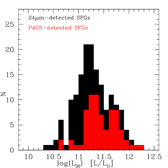
Figure 9: Distribution of $L_{IR}$ over the sample of SFGs with at least a 24 $\mu m$ detection (black histogram). The red histogram shows the $L_{IR}$ distribution of PACS-detected sources only.

The infrared luminosities can be converted into SFR using the Kennicutt (1998) relation:

$$SFR_{IR}(M_{\odot}yr^{-1})=2.9\times 10^{-44}L_{IR}(erg/s),$$ (1)

In star-forming galaxies $SFR_{IR}$ is expected to be a good estimate of the total SFR. However, there might be a fraction of UV radiation that escapes dust absorption and that is not incorporated into the calibrations. This missing unattenuated component varies from essentially zero in dusty starburst galaxies to nearly 100$\%$ in dust-poor dwarf galaxies and metal-poor regions of more-massive galaxies (Kennicutt & Evans 2012). To overcome this bias many authors suggest adding another term to $SFR_{IR}$ to account for the unobscured UV light (Papovich et al. 2007; Rodighiero et al. 2010a; Wuyts et al. 2011; Nordon et al. 2013; Kennicutt & Evans 2012). This second term is simply the SFR derived from UV luminosity, not corrected for dust extinction. We adopted the appropriate relation from Kennicutt (1998),

$$SFR_{UV}(M_{\odot}yr^{-1})=0.9\times 10^{-28}L_{\nu}(1500\AA)(ergs^{-1}Hz^{-1}),$$ (2)

and finally define

$$SFR_{IR+UV}{=}SFR_{IR}+SFR_{UV}$$ (3)

as total SFR (obscured plus un-obscured) (Wuyts et al. 2011; Nordon et al. 2013).

In Fig. 10 we plot the total SFR ($SFR_{IR+UV}$) vs. the IR component alone. The contribution of $SFR_{UV}$ to the total SFR is almost negligible in ultra-luminous (ULIRGs: $L_{IR}{/}L_{\odot}{\geq}10^{12}$) and the majority of luminous (LIRGs: $10^{11}{<}L_{IR}{/}L_{\odot}{<}10^{12}$) IR galaxies, while in normal SFGs ($L_{IR}{/}L_{\odot}{\leq}10^{11}$) its contribution to the total SFR grows to about $30\%$. However, we have tested how neglecting this contribution would alter our results and we found that none of the calibrations derived in this paper would significantly change if $SFR_{IR}$ were assumed as total SFR, instead of $SFR_{IR+UV}$.

In the following sections we shall compare $SFR_{IR+UV}$ to the other SFR estimators available for our sample, with particular emphasis on spectroscopic data. Using the IR data to calibrate UV and optical estimators, we can derive a set of relations that can be used to consistently compare galaxies in a wide range of redshifts ($1{<}z{<}3$) and with different kinds of available data (from observed optical photometry and spectra, to IR data).

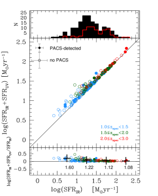
Figure 10: Main plot: comparison between $SFR_{IR+UV}$ and $SFR_{IR}$ for SFGs with at least one IR detection. Filled points mark PACS-detected galaxies. Bottom plot: $SFR_{IR+UV}$ over $SFR_{IR}$ ratio as a function of $SFR_{IR}$. Median ratio in bins of $SFR_{IR}$ are also shown. Upper plot: black histogram is the distribution of $SFR_{IR}$ over the entire sample of SFGs; red empty histogram is the distribution of PACS-detected sources only.

5 Dust-extinction correction: SFR from UV continuum luminosity

The UV luminosity emitted by young stars is a direct indicator of ongoing star formation. However, it is typically severely extincted by the dust surrounding star-forming regions, therefore the measured rest-frame UV luminosity must be corrected before being converted into SFR. Empirical relations are usually applied for this purpose, most of them calibrated on local galaxies.

5.1 UV sample: SFGs at $1.6{<}z{<}3$

In galaxies dominated by a young stellar population, the shape of the UV continuum can be fairly accurately approximated by a power law $F_{\lambda}{\varpropto}\lambda^{\beta}$, where $F_{\lambda}$ is the observed flux ($erg\leavevmode\nobreak\ s^{-1}\leavevmode\nobreak\ cm^{-2}\leavevmode\nobreak\ \AA^{-1}$) and $\beta$ is the continuum slope (Calzetti et al. 1994). Meurer et al. (1999) found, for a sample of local starburst galaxies, a correlation between the UV spectral slope ($\beta$) and the ratio of $L_{IR}$ over UV luminosity ($L_{UV}=\nu L_{\nu}(1500\AA)$), not corrected for extinction, which can be translated into attenuation $A_{1600\leavevmode\nobreak\ \AA}$. Overzier et al. (2011) and Takeuchi et al. (2012) independently revised the original Meurer et al. (1999) relation correcting for the effect of the small IUE aperture used in the original calibration, thanks to GALEX data, and using an update estimate for $L_{IR}$ (total IR emission instead of IRAS far-IR (FIR) emission in the range $40-120\mu m$). The attenuation vs. $\beta$ relation has since been used for galaxies at various redshifts, though different studies have reported contradicting results about its general validity (Calzetti 2001; Boissier et al. 2007; Seibert et al. 2005; Reddy et al. 2010; Overzier et al. 2011; Reddy et al. 2012; Takeuchi et al. 2012; Buat et al. 2012; Heinis et al. 2013; Nordon et al. 2013; Castellano et al. 2014; Oteo et al. 2013, 2014). Here we tested the relation for our sample using $L_{IR}$ derived from our mid- and far-IR photometry, in order to obtain an estimate of SFR from dust-corrected UV flux consistent with the one from IR+UV defined in the previous section.

The attenuation is defined from the ratio between $L_{IR}$ and uncorrected $L_{UV}$ ($IRX=L_{IR}/L_{UV}$). However, the exact definition is not unique across the literature (Meurer et al. 1999; Buat et al. 2005). Here we adopt the definition (Nordon et al. 2013)

$$log(SFR_{IR+UV})=log(SFR_{UV})+0.4\leavevmode\nobreak\ A_{IRX}$$ (4)

$$A_{IRX}\leavevmode\nobreak\ =\leavevmode\nobreak\ 2.5\leavevmode\nobreak\ log\left(\frac{SFR_{IR}}{SFR_{UV}}\leavevmode\nobreak\ +\leavevmode\nobreak\ 1\right),$$ (5)

where $SFR_{UV}$ is the uncorrected quantity, as defined in Sec. 4, and $SFR_{IR+UV}$ is the total SFR. This definition is consistent with the ones adopted by Overzier et al. (2011) and Takeuchi et al. (2012).

The slope $\beta$ is defined in the wavelength range from ${\sim}1250{\AA}$ to ${\sim}2600{\AA}$ (Calzetti et al. 1994), and can be measured either directly on spectra or by using photometry. In our sample, only galaxies in the UV sample have spectra with the right wavelength coverage; for the [OII] sample photometry has to be used.

The 62 IR-detected galaxies with a measurable spectral slope were then used to test the $A_{IRX}$ vs. $\beta$ relation at $1.6{<}z{<}3$ and the result is shown in Fig. 11. The continuum slope of each spectrum was derived through a linear fit of the average fluxes in the spectral windows defined by Calzetti et al. (1994), in the $log(F_{\lambda})-log(\lambda)$ plane. More details about the spectroscopic determination of $\beta$ can be found in the Appendix.

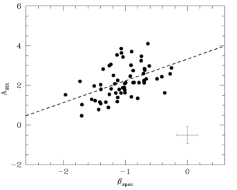
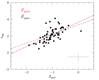
Figure 11: $A_{IRX}$ vs. $\beta$ for IR-detected galaxies in the UV sample. Top: $\beta$ is measured from the spectra. The black line is a fit to the data (Eq.6). Bottom: $\beta$ is measured from photometry. The red line is a fit to the data (Eq.7). The black line is the relation for $\beta_{spec}$.

We then derive the best-fit relation by performing a linear fit of the form $A_{IRX}=C_{0}\times\beta+C_{1}$ to the data,

$$A_{IRX}\leavevmode\nobreak\ =\leavevmode\nobreak\ (1.10\pm 0.23)\times\beta_{spec}+(3.33\pm 0.24)$$ (6)

with an r.m.s. dispersion of the residuals ${\sim}0.7$.

Our relation ($C_{0}{=}1.10$) is broadly consistent with the one by Murphy et al. (2011) for a sample of $24\mu$m-detected galaxies at $z{\sim}2$ ($C_{0}{=}0.75$). On the other hand, it is flatter than in the UV-selected samples of Overzier et al. (2011) (local) and Buat et al. (2012) ($z{\sim}1.5$) (respectively, $C_{0}{=}1.96$ and $C_{0}{=}1.70$). Also, the standard deviation in the latter cases is of the order of $\sim$0.3 dex, while our relation is more dispersed. We ascribe it mainly to the different sample selections. A low dispersion is expected when galaxies are UV-selected local starbursts or high-redshift equivalents, but deviations from a tight relation have been reported both for dusty IR-luminous galaxies and for quiescently star-forming galaxies (Buat et al. 2012; Takeuchi et al. 2012, and references therein). Our parent catalogue is mass-selected, therefore our sample is expected to include objects with a wide range of star formation histories and different levels of starburst activity that may be characterized by different attenuation laws and increase the scatter in the relation, with respect to a UV selection. In particular, we found that the objects that deviate the most from our relation (i.e. with the highest $A_{IRX}$ at fixed $\beta$) have the highest $L_{IR}$.

The continuum slope can be derived also from photometric data, either by measuring $\beta$ directly from the best-fit SED template to the overall photometric data of the galaxy (e.g. Oteo et al. 2013, 2014), or by fitting the photometric points which sample the UV continuum at the redshift of the galaxy with a power-law function (e.g. Bouwens et al. 2009; Buat et al. 2012; Nordon et al. 2013; Pannella et al. 2015). We decided to use the latter method, to avoid model dependencies. Uncertainties were computed by randomizing the observed fluxes according to their errors and repeating the fit to derive a new slope. Since even with the photometry we cannot probe wavelengths as short as ${\sim}1200\AA$ at $z{\sim}1$, for the photometric determination of the continuum slope we decided to use, at all redshifts, a shorter rest-frame wavelength range to derive $\beta_{phot}$, starting from $\lambda_{rest}{\sim}1500\AA$. This wavelength coverage is also the most popular in the literature, when the slope is derived from photometry and not from spectra (see e.g. Bouwens et al. 2009, 2012; Nordon et al. 2013; Castellano et al. 2012).

We computed $\beta_{phot}$ in the UV sample for the same galaxies for which $\beta_{spec}$ had been already derived and a similar relation was found between $\beta_{phot}$ and $A_{IRX}$,

$$A_{IRX}\leavevmode\nobreak\ =\leavevmode\nobreak\ (1.45\pm 0.25)\times\beta_{phot}+(3.63\pm 0.26),$$ (7)

with an r.m.s. dispersion of the residuals ${\sim}0.6$. This relation gives attenuation values that are consistent with those derived from spectroscopy. This result will justify us to use the photometric slope to derive a similar relation for the galaxies in the [OII] sample, where the spectra do not cover the wavelength range needed to compute $\beta$.

5.2 A little digression about regression methods

Since our aim is to provide a relation to predict the value of a variable from the measurement of another, we adopted an OLS (Y$|$X) fit in the derivation of the $A_{IRX}$ vs. $\beta$ relation. The OLS (Y$|$X) fit is the most widely used in the literature and we are assuming that ”OLS” and ”linear regression”, in the absence of further specification, means OLS (Y$|$X) in all the works whose calibrations we cite here to compare with our findings.

A fit that treats symmetrically the two variables is instead to be preferred when the goal is to estimate the underlying functional relation between the variables (Isobe et al. 1990). The slope of the $A_{IRX}$ vs. $\beta$ relation ($C_{0}$) depends on the attenuation curve. The $C_{0}$ parameter expected from a given attenuation curve should be compared to the value derived from a symmetric fit, instead of an OLS (Y$|$X). We report that an OLS bisector fit (Isobe et al. 1990) to the data analysed in Fig. 11 (top) would produce the following relation (see Eq. 6 for the corresponding OLS (Y$|$X) fit)

$$A_{IRX}\leavevmode\nobreak\ =\leavevmode\nobreak\ (1.96\pm 0.23)\times\beta_{spec}+(4.22\pm 0.19)\ \ \ \ \ [OLSBisector],$$ (8)

while in the case of $\beta_{phot}$ (Fig. 11 bottom) we would have

$$A_{IRX}\leavevmode\nobreak\ =\leavevmode\nobreak\ (2.16\pm 0.27)\times\beta_{phot}+(4.36\pm 0.27)\ \ \ \ \ \ [OLSBisector],$$ (9)

whose corresponding OLS (Y$|$X) fit is given in Eq. 7. For comparison, the $C_{0}$ value expected from the Calzetti law is $C_{0}{=}2.3$, which gives a relation fairly consistent with our findings.

5.3 Extinction from observed colour

Another popular empirical recipe to derive a dust extinction correction to be applied to UV fluxes, for galaxies at $z{\geq}1.4$, comes from the tight correlation that Daddi et al. (2004) found between the observed $(B-z)$ colour and $E(B{-}V)$ of BzK galaxies. This relation is valid only for galaxies in the redshift range $1.4{<}z{<}2.5$, where the $(B-z)$ colour is basically another way of expressing the UV continuum slope. In the Daddi et al. (2004) paper, the $E(B{-}V)$ is derived from SED fitting to UV-to-NIR (near-IR) multi-band photometry (assuming Bruzual & Charlot (2003) models, Salpeter IMF, constant star formation, and a Calzetti law).

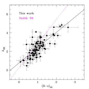
Figure 12: $A_{IRX}$ vs. the (B-z) colour. Black line is a fit to the data. The magenta line is the Daddi et al. (2004) relation, plotted as reference.

In this work we use instead the available IR data to calibrate the $(B-z)$ colour as an extinction estimator. A linear fit to the data produces the following relation:

$$A_{IRX}\leavevmode\nobreak\ =\leavevmode\nobreak\ (1.64\pm 0.13)\times(B-z)_{AB}+(0.77\pm 0.13).$$ (10)

In Fig. 12 we plot all IR-detected SFGs at $1.4{<}z{<}2.5$. The original Daddi et al. (2004) relation is shown as a reference. The two relations are in general quite consistent, but ours is flatter for galaxies with reddest (B-z).

The attenuation derived from $(B-z)$ colour is consistent with the one derived from the continuum slope in the previous section, not only for the IR-detected galaxies (that were actually used to derive both sets of calibrations), but also for galaxies without IR information.

5.4 [OII] sample: SFGs at $1{<}z{<}1.6$

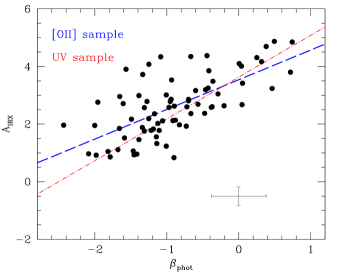
Figure 13: $A_{IRX}$ vs. $\beta_{phot}$ for IR-detected galaxies in the [OII] sample. The blue line is a fit to the data (Eq. 11). The red line is the $A_{IRX}$ vs. $\beta_{phot}$ relation for the UV sample (Eq. 7).

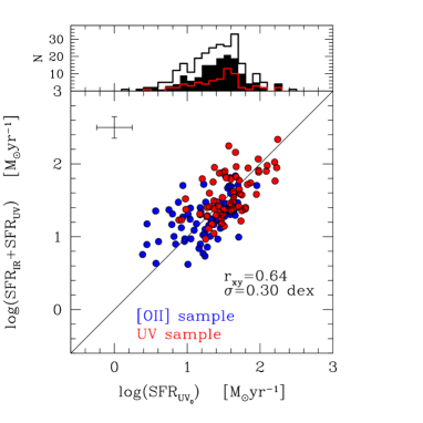
Figure 14: Main plot: comparison between $SFR_{IR+UV}$ and $SFR_{UV_{0}}$ corrected using the $A_{IRX}$ vs. $\beta$ relations derived in the paper. $\beta$ is derived from spectroscopy, when possible, otherwise from photometry (see the text for more details). Upper plot: black empty histogram is the distribution of $SFR_{UV_{0}}$ over the entire sample of SFGs; black filled histogram is the distribution of $SFR_{UV_{0}}$ over the sample of 24 $\mu m$-detected sources (both with and without PACS data); red empty histogram is the distribution of PACS-detected sources only.

In our sample, only galaxies in the UV sample have spectra with the right wavelength coverage to compute the continuum slope. However, photometry can also be used for the same task. For the galaxies in the [OII] sample we computed the slope $\beta_{phot}$ between $\sim$1500$\AA$ and $\sim$2600$\AA$, as explained in the previous section, and we found the following relation with $A_{IRX}$,

$$A_{IRX}\leavevmode\nobreak\ =\leavevmode\nobreak\ (1.03\pm 0.26)\times\beta_{phot}+(3.54\pm 0.25),$$ (11)

with an r.m.s. dispersion of the residuals is ${\sim}0.8$ (Fig. 13). Comparing Eq. 7 and Eq. 11 we find that in the [OII] sample the slope of the relation ($C_{0}$) is slightly flatter than in the UV sample. However, the difference is not highly significant, therefore we see no evolution of the $A_{IRX}$ vs. $\beta$ relation between $z{\sim}1.3$ and $z{\sim}2.3$. Moreover, dust attenuation of the galaxies in both samples broadly follows the prediction of the Calzetti law (when considering the OLS bisector relations; see Sec. 5.2), though in the low-redshift bin the Calzetti law tends to over-predict the attenuation in objects with the reddest slope, with respect to the results of our calibrations (see also Pannella et al. 2015).

The relations derived in this and the previous sections were applied to all the galaxies in our sample, choosing the appropriate one for each object to derive $A_{IRX}$ values from the UV continuum slope and compute the un-extincted SFR ($SFR_{UV_{0}}$). The final check to assess how good the calibrations are to recover the total SFR comes from the comparison between $SFR_{UV_{0}}$ and $SFR_{IR+UV}$ in Fig. 14 where we can see that the two estimates are in good agreement.

6 Dust-extinction correction: SFR from [OII]$\lambda$3727 emission line luminosity

The next SFR estimator to be considered was the forbidden line [OII]$\leavevmode\nobreak\ \lambda 3727$. The luminosities of forbidden lines are not directly coupled to the ionizing luminosity, and their calibration as SFR indicators is sensitive to density variations in dust reddening, chemical abundance, and ionization among star-forming galaxies (Kennicutt 1998; Jansen et al. 2001; Kewley et al. 2004; Moustakas et al. 2006). The excitation of [OII]$\lambda$3727 is sufficiently well behaved that it can be calibrated empirically as a quantitative SFR tracer through H$\alpha$, though the [OII]/H$\alpha$ ratio in individual galaxies can vary considerably and this is the main uncertainty related to the [OII]-derived estimate of SFR. The other two major sources of uncertainty are the effects of metallicity and dust extinction on the conversion of [OII]$\lambda$3727 luminosity into SFR.

Various approaches have been proposed in the literature to derive dust-corrected estimates of $SFR_{[OII]_{0}}$. Kewley et al. (2004), for example, derive a local $SFR_{[OII]_{0}}$ calibration based on the intrinsic (e.g. reddening corrected) [OII]$\lambda$3727 luminosity and the abundance. The local calibration by Moustakas et al. (2006) is instead parametrized in terms of the B-band luminosity to remove the systematic effects of reddening and metallicity. Both calibrations use as reference SFR the estimate from H$\alpha$ luminosity, corrected for dust-extinction using the Balmer decrement.

6.1 The [OII]$\lambda$3727 equivalent width vs. $\beta$ relation

Here we exploit the Spitzer-Herschel data and use $SFR_{IR+UV}$ as reference to calibrate a dust-corrected estimate of SFR from [OII]$\lambda$3727 luminosity for our [OII] sample of galaxies at $1.0{<}z{<}1.6$.

Integrated line fluxes of [OII]$\lambda$3727 were measured and corrected for slit-losses using the available photometry. We assume the Kennicutt (1998) calibration (scaled to a Kroupa IMF) to convert [OII]$\lambda$3727 luminosity into SFR,

$$SFR_{[OII]_{0}}(M_{\odot}yr^{-1})=0.9\times 10^{-41}L_{[OII]_{0}}(ergs^{-1}),$$ (12)

where $L_{[OII]_{0}}$ is the intrinsic [OII]$\lambda$3727 luminosity, corrected for dust extinction. We explored the possibility of calibrating a relation between attenuation, derived by our IR data, and some property of the [OII]$\lambda$3727 line, in order to obtain a self-consistent way of computing the dust corrected $SFR_{[OII]_{0}}$ from [OII]$\lambda$3727 information alone, without the aid of additional multi-wavelength photometric data. An anti-correlation ($r_{xy}{=}-0.56$) was found between the rest-frame equivalent width (EW) of the [OII]$\lambda$3727 line (i.e. the blended doublet) and the UV continuum slope (Fig. 15), both for galaxies with and without IR data.

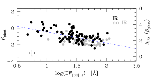
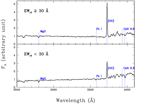
Figure 15: Top: $\beta_{phot}$ vs. log($EW_{[OII]}$) rest-frame. We use the convention of positive EW for emission lines. The right axis converts $\beta_{phot}$ to $A_{IRX}$ using Eq. 11. Black points represent IR-detected galaxies, while grey points represent galaxies with no IR detection. The blue dashed line is a linear fit to the points. Bottom: average spectra in two bins of rest-frame $EW_{[OII]}$. Lines of interest are labelled.

A linear fit gives the relation

$$\beta_{phot}\leavevmode\nobreak\ =\leavevmode\nobreak\ (-1.35\pm 0.20)\leavevmode\nobreak\ \times\leavevmode\nobreak\ log(EW_{rest})\leavevmode\nobreak\ +\leavevmode\nobreak\ (0.91\pm 0.30)$$ (13)

with an r.m.s. dispersion of the residuals ${\sim}0.6$. Since $\beta$ is related to dust attenuation (Eq. 11), the relation with EW implies a relation between EW and dust attenuation for the galaxies in our sample. Combining Eq. 11 and Eq. 13 we obtain

$$A_{IRX}\leavevmode\nobreak\ =\leavevmode\nobreak\ (-1.39\pm 0.26)\leavevmode\nobreak\ \times\leavevmode\nobreak\ log(EW_{rest})\leavevmode\nobreak\ +\leavevmode\nobreak\ (4.48\pm 0.35),$$ (14)

Despite all our efforts to clean the sample from galaxies in which older stellar populations might contribute to dust heating (i.e. $L_{IR}$) and continuum reddening, we cannot completely exclude a mild contribution that might increase the scatter in the $\beta_{phot}$ vs. $log(EW_{rest})$ relation in the low-EW_[OII] part of the sample, given the presence of Balmer absorption lines (stronger in A-type stars) and CaII $H{\&}K$ lines in the low-EW_[OII] stacked spectrum (Fig. 15). On the other hand, we measure a stronger EW of the MgII$\lambda$2800 ISM absorption line (i.e. the blended doublet) in the low-EW_[OII] stacked spectrum (Fig. 16): ISM absorption lines have been observed to be stronger in SFGs with redder $\beta$ and characterized by higher dust extinction (Shapley et al. 2003; Talia et al. 2012).

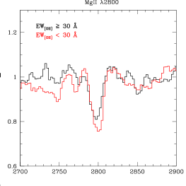
Figure 16: Composite spectra of galaxies in the [OII] sample in two bins of rest-frame $EW_{[OII]}$: zoomed-in image of the MgII$\lambda$2800 ISM absorption line.

6.2 Continuum vs. nebular attenuation

We cannot use directly $A_{IRX}$ derived in Eq. 14, i.e. the attenuation towards the continuum, to correct the [OII]$\lambda$3727 luminosity, first because of its dependency on wavelength, and second because of the extra amount of reddening suffered by nebular emission, with respect to the continuum, claimed by many authors starting from Calzetti (1997). The first point means that an extinction curve must be assumed. It is known that the effects of dust are stronger at shorter wavelengths, therefore correcting a luminosity measured at $\lambda$3727$\AA$ using an attenuation measured at $\lambda$1500$\AA$ would produce an over-correction. The extra reddening towards nebular lines is an issue still strongly debated. In fact, though many authors have confirmed the original findings by Calzetti (1997); Calzetti et al. (2000) also at high redshift (see e.g. Förster Schreiber et al. 2009; Wuyts et al. 2011), other studies claim a ratio between continuum and nebular attenuation much closer to unity (Reddy et al. 2010; Kashino et al. 2013; Pannella et al. 2015; Puglisi et al. 2015).

To summarize, the dust extinction corrected SFR is

$$SFR_{[OII]_{0}}(M_{\odot}yr^{-1})=0.9\times 10^{-41}L_{[OII]}\times 10^{0.4A_{[OII]}}(ergs^{-1}),$$ (15)

where $L_{[OII]}$ is the observed, uncorrected [OII]$\lambda$3727 luminosity. If we parametrize the extra reddening as

$$E(B-V)_{neb}=E(B-V)_{cont}/f$$ (16)

and assume a reddening curve ($\kappa_{\lambda}$), then $A_{[OII]}$ is defined as

$$A_{[OII]}=A_{IRX}\times(\kappa_{H_{\alpha}}/\kappa_{1500\AA})\times f^{-1}.$$ (17)

We use the value of the extinction curve at H$\alpha$ as prescribed by Kennicutt (1998) because of the manner in which the [OII]$\lambda$3727 luminosities were calibrated through the [OII]/H$\alpha$ ratio.

In the UV regime a Calzetti et al. (2000) law is a fair assumption for the reddening curve, for our sample. In the optical range with our data we are unable to constraint the reddening curve and we decided to assume the same Calzetti et al. (2000) law to ease the comparison with recent works on differential attenuation (e.g. Kashino et al. 2013; Wuyts et al. 2013; Price et al. 2014), though it is still unclear if this is an appropriate assumption in the context of high-redshift galaxies (Reddy et al. 2015).

We derive dust extinction corrected $SFR_{[OII]_{0}}$ assuming different values of f and compare the result to $SFR_{[UV]_{0}}$ (corrected using $\beta_{phot}$ and Eq. 11) to derive an estimate of the best f-factor. The best agreement is found with $f{=}0.50$, which is very close to the 0.59 value quantified by Calzetti (1997). In Fig. 17 where we also plot, for comparison, the fits corresponding to other two different choices of f (0.75 and 1.0). The small dispersion (${\sim}0.2$) is due to the correlation of the corrections on the two axes, since we derive $A_{[OII]}$ from $A_{IRX}$. Though we cannot draw any conclusive statement, our data appear to be more consistent with the need of an extra attenuation towards nebular lines in galaxies at high redshift, than with studies that claim an f coefficient much closer to unity.

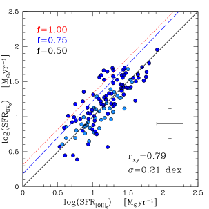
Figure 17: $SFR_{UV_{0}}$ vs. $SFR_{[OII]_{0}}$ corrected for dust extinction using, respectively, $\beta_{phot}$ and Eq. 11, and $EW_{[OII]}$ and Eq. 14 assuming a Calzetti et al. (2000) law and $f{=0.50}$. The black line is the 1-to-1 relation that also corresponds also to a linear fit to the points. Blue and red lines show the fits with other two different assumptions of $f$. Blue points are IR-detected galaxies, while light blue points are galaxies with no IR detection.

We stress that the relevant relation that we derive in this work is the one linking $\beta_{phot}$ and $EW_{[OII]}$. Then, the actual attenuation of the [OII]$\lambda$3727 line luminosity depends on the $(\kappa_{H_{\alpha}}/\kappa_{1500\AA}){\times}f^{-1}$ term in Eq. 17, i.e. on the combination of the assumptions about the reddening laws respectively for the stellar continuum and nebular emission, and the best f value that we derive by forcing agreement between $SFR_{[OII]_{0}}$ and our reference SFR. With this approach, different assumptions about the reddening law will produce different estimates of f (Puglisi et al. 2015), but the resulting $SFR_{[OII]_{0}}$ values will be always, by construction, consistent with one another.

As an exercise we derived the f value under a different assumption for the nebular attenuation law. We choose a Galactic extinction curve, consistently with the original prescription by Calzetti (1997), in particular the Cardelli et al. (1989) one, while for the stellar continuum we continued to assume the Calzetti et al. (2000) law (Reddy et al. 2015; Steidel et al. 2014). With this choice of attenuation curves the best agreement between $SFR_{[OII]_{0}}$ and $SFR_{[UV]_{0}}$ is found with $f{=}0.37$.

To conclude this section we summarize the steps to derive the dust extinction corrected $SFR_{[OII]_{0}}$:

1. Derive the attenuation towards the continuum ($A_{IRX}$) from the rest-frame $EW_{[OII]}$ and its relation with $\beta_{phot}$ (Eq. 13-14).

2. Convert $A_{IRX}$ into $A_{[OII]}$ assuming appropriate reddening curves respectively for the stellar continuum and nebular emission, and an extra-attenuation factor (Eq. 17).

   In this work we assume a Calzetti et al. (2000) law for both the stellar continuum and nebular emission and apply an $f$-factor $f{=}0.50$. If a Cardelli et al. (1989) Galactic extinction curve were instead applied to nebular emission, while keeping the Calzetti law for the stellar continuum, the $f$-factor to be used would be $f{=}0.37$.

3. Derive $SFR_{[OII]_{0}}$ by correcting the observed [OII]$\lambda$3727 line luminosity with $A_{[OII]}$ (Eq. 15); in this work we assume a Kennicutt (1998) calibration.

Finally, we are aware that our relations are taking the calibration of the [OII]$\lambda$3727 line as a SFR indicator as a closed box because with the data in our possess we cannot tackle the issue of how the [OII]/H$\alpha$ ratio varies across our sample, as a function of different gas properties. For this reason our method for deriving the $SFR_{[OII]_{0}}$ should be applied carefully to individual galaxies. However, our calibration will be useful for computing the statistical star formation and extinction properties of large high-redshift galaxy samples, when no other information about nebular extinction is available.

7 A quick look at SFR from SED fitting

We dedicate a brief section to the SFR estimate derived by fitting the galaxy UV-to-NIR broad-band photometry to the spectral energy distribution (SED) of synthetic stellar populations. For this exercise we do not consider the FIR data but use only photometry from U band to IRAC 5.8$\mu$m, to see how the results of our calibrations compare to a different dust-corrected SFR estimate derived without direct information on dust emission.

A widespread approach is to use models in which the star formation history (SFH) is described by an exponentially declining SFR, though in the last years some studies have introduced increasing star formation histories as a better way to describe high-redshift star-forming galaxies, namely at $z{\sim}2$ (Maraston et al. 2010; Reddy et al. 2012). We choose the set of models by Maraston (2005) and used the HyperZ software (Bolzonella et al. 2000) to perform the SED fitting. star formation histories were parametrized by exponentials ($e^{-t/\tau}$) with e-folding timescale $\tau$ between 100 Myr and 30 Gyr, plus the case of constant SFR. We assumed a Kroupa IMF, fixed solar metallicity, a Calzetti law for dust extinction, and a minimum age $age_{min}{=}0.09\leavevmode\nobreak\ Gyr$. We derived from simulations the errors on the quantities estimated using SED fitting techniques. We found that errors on both $SFR_{SED}$ and stellar masses are, on average, ${\sim}\leavevmode\nobreak\ 30\%$ (Bolzonella, private communication).

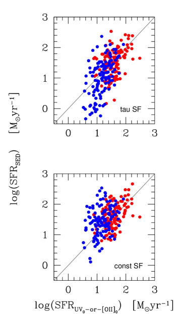
Figure 18: Comparison between $SFR_{SED}$ and SFR estimated from spectroscopic tracers: UV flux, corrected using $\beta$, for galaxies in the UV sample (red points), and [OII]$\lambda$3727 flux, corrected using EW_[OII], for galaxies in the [OII] sample (blue points).

In Fig. 18 (top) we compare the results from SED fitting, under the cited assumptions, to the ones previously obtained from our calibrations. In particular, for the UV sample we plot $SFR_{UV_{0}}$ corrected using $\beta$, while for the OII sample we plot $SFR_{[OII]_{0}}$ corrected as explained at the end of Sec. 6.2 (assuming a Calzetti law for both stellar continuum and nebular emission and applying an extra-attenuation $f{=}0.50$). There is a general fair agreement between the two estimates at high SFR, but in the low-SFR regime the SED estimate is lower than our calibrated values, i.e. lower than $SFR_{IR+UV}$ on which our calibrations are based. This tail at low $SFR_{SED}$ has been reported also by other authors (Wuyts et al. 2011; Reddy et al. 2012; Arnouts et al. 2013; Utomo et al. 2014), according to which this difference may have multiple causes. Either IR+UV is overestimating the true SFR due to a non-negligible contribution of old stars to the dust heating or some of the physical assumptions made in the SED fitting procedure do not correctly describe the analysed galaxies, causing $SFR_{SED}$ to underestimate the true SFR. In our case, we tend to exclude the former explanation because we specifically excluded galaxies showing evidence of old stellar populations in their spectra. To investigate thoroughly if and how degenerate SED fitting parameters (i.e. SFH, age, attenuation law, metallicity) should be tuned in order to recover the true SFR is beyond the scope of this work. Therefore we limited ourselves to a quick test and we changed only one of the main assumptions, namely the SFH, by forcing all galaxies to a constant SF (and leaving all the other parameters unchanged). We note that, in our sample, when $\tau$ is left as a free parameter only for $\sim 20\%$ of the galaxies the best $\chi^{2}$ is obtained with a constant star formation history. The results are shown in Fig. 18, bottom plot. Assuming a constant SFH the less star-forming galaxies are forced to values of their $SFR_{SED}$ that are in better agreement with our calibrated estimate with respect to the results obtained by leaving $\tau$ a free parameter (see also Wuyts et al. 2011), though especially in the $[OII]sample$ $SFR_{SED}$ seems to be systematically slightly higher than our IR-calibrated values.

8 An application: the SFR vs. Mass relation

An obvious application of the calibrations derived in the previous section is the study of the SFR vs. stellar mass relation.

The SFR-M_⋆ relation is expected to evolve with redshift (Daddi et al. 2007; Noeske et al. 2007; Wuyts et al. 2011; Whitaker et al. 2012; Heinis et al. 2013; Buat et al. 2014), therefore we divided our sample into three redshift bins, each spanning ${\sim}1.2$ Gyrs (Fig. 19). The SFR for each galaxy is chosen as follows: $SFR_{IR+UV}$ for IR-detected galaxies and the appropriate IR-calibrated SFR estimate ($SFR_{[OII]_{0}}$ or $SFR_{UV_{0}}$) for galaxies not detected in IR, depending on the redshift. Stellar masses were computed using Maraston (2005) models with the assumptions outlined in the previous section and constant SF.

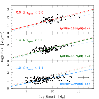
Figure 19: SFR vs. Mass in three redshift bins, each spanning ${\sim}1.2$ Gyrs. For each galaxy, the plotted SFR estimate is $SFR_{IR+UV}$ for IR-detected galaxies and $SFR_{[OII]_{0}}$ or $SFR_{UV_{0}}$ for galaxies with no IR data respectively in the [OII] sample and in the UV sample. In each panel the three lines are the fits (OLS bisector) to the data in the three redshift bins. Different colours identify each redshift bin.

We find that our galaxies lie on a close linear relation with $\sigma{\sim}0.3$ dex and $r_{xy}{\sim}0.6$ at all redshifts. There are weak trends both for the slope and the normalization, with the slope becoming steeper and the normalization higher with increasing redshift, though the completeness limits and spectroscopic requirements of our sample do not allow a robust qualification. However, we note that the dispersion that we find in the relation is consistent with that often quoted in the literature (see e.g. Daddi et al. 2007; Noeske et al. 2007; Whitaker et al. 2012; Buat et al. 2014). Also, the same trend of the normalization with redshift has been reported in previous works, while there is not a consensus yet on the evolution of the slope with redshift (Elbaz et al. 2007; Noeske et al. 2007; Whitaker et al. 2012; Heinis et al. 2013; Buat et al. 2014; Pannella et al. 2015), as an effect of different sample selections, completeness limits and chosen SFR estimators. In the redshift range $1{<}z{<}3$ literature quoted values of the slope range from $\sim$0.7 to $\sim$0.9 (see also Wuyts et al. 2011; Rodighiero et al. 2011; Kashino et al. 2013; Rodighiero et al. 2014), with which our findings are consistent.

9 Conclusions and summary

In this paper we use a sample of galaxies drawn from the GMASS survey to study different SFR estimators. Our aim is to use IR data to derive empirical calibrations to correct UV and [OII]$\lambda 3727$ luminosities for dust extinction. To do this, we concentrated on a well-controlled spectroscopic sample, rich of ancillary data.

Table 4: Summary table of all the relations derived in the paper. For each relation, observed and derived quantities are indicated, as well as slope and intercept of the linear relation, with associated uncertainties. Relations are given in the form: $Derived=Slope\times Observed+Intercept$.

Observed	Derived	Slope	Intercept	z	Notes	Sec.
$\beta_{spec}$	$A_{IRX}$	1.10 $\pm$ 0.23	3.33 $\pm$ 0.24	$1.6{<}z{<}3.0$	spectral coverage: $1200-2600\AA$	5.1, A
$\beta_{phot}$	$A_{IRX}$	1.45 $\pm$ 0.25	3.63 $\pm$ 0.26	$1.6{<}z{<}3.0$		5.1
(B-z)	$A_{IRX}$	1.64 $\pm$ 0.13	0.77 $\pm$ 0.13	$1.4{<}z{<}2.5$		5.3
$\beta_{phot}$	$A_{IRX}$	1.03 $\pm$ 0.26	3.54 $\pm$ 0.25	$1.0{<}z{<}1.6$		5.4
log($EW_{[OII]}$)	$\beta_{phot}$	-1.35 $\pm$ 0.20	0.91 $\pm$ 0.30	$1.0{<}z{<}1.6$	$[OII]\lambda 3727$ emission line	6.1
log($EW_{[OII]}$)	$A_{IRX}$	-1.39 $\pm$ 0.26	4.48 $\pm$ 0.35	$1.0{<}z{<}1.6$	$[OII]\lambda 3727$ emission line	6.1

We started by selecting a sample of SFGs with a spectroscopic redshift $1{<}z{<}3$ from a pure magnitude-limited parent sample ($\emph{m}_{4.5}{<}23.0$). In the chosen redshift range this selection is most sensitive to stellar mass. In particular, the limiting mass sensitivities are $log(M/M_{\odot})\sim$ 9.8, 10.1, and 10.5 for $z=$ 1.4, 2, and 3, respectively. Our sample can be divided into two sub-samples with homogeneous rest-frame wavelength coverage:

• galaxies at $1{<}z{<}1.6$ that cover the range $\sim 2700-4300\AA$ ([OII] sample), where the [OII]$\lambda$3727 emission line can be observed;

• and galaxies at $1.6{<}z{<}3$ that cover the range $\sim 1100-2800\AA$ (UV sample), in whose spectra strong ISM absorption lines can be detected.

We excluded from the sample all quiescent galaxies and AGNs, identified on the basis of spectroscopic features and X-ray luminosity. We also used three continuum indices (MgUV, C(29-33), D4000) to clean the resulting preliminary selection of SFGs from galaxies showing some evidence of the presence of old stellar populations that could bias the correct interpretation of the dust- and SFR-related observables. The final sample includes 286 SFGs, of which on third has IR information coming from Spitzer-MIPS and Herschel-PACS, and another one third has only a Spitzer-MIPS detection.

Though inevitably not complete, especially due to the spectroscopic requirement that introduces a bias towards brighter and bluer objects, our sample is fairly representative of a specific galaxy population whose properties may be summarized as follows:

• redshift between $z\sim 1$ and $z\sim 3$;

• intermediate stellar mass (approximately in the range $10^{9.2}{<}M/M_{\odot}{<}10^{10.2}$);

• blue rest-frame colours: $(NUV-r){<}3\ \&\ (r-K){<}1.4$ or
  $(U-V){<}1.2\ \&\ (V-J){<}1.5$;

The bolometric IR luminosity, $L_{IR}$, was derived for all IR-detected galaxies, using the most up-to-date models, i.e. SED fitting to U-to-FIR broad-band photometry with Magphys (da Cunha et al. 2008) for PACS-detected galaxies, and 24$\mu$m-to-bolometric $L_{IR}$ correction using main sequence SED models by Magdis et al. (2012) for MIPS-detected galaxies with no PACS data. $L_{IR}$ values were then converted to SFR, to which we added a second component accounting for unobscured SFR, in order to recover the total SFR ($SFR_{IR+UV}$). Assuming $SFR_{IR+UV}$ as our benchmark SFR estimate, we derived some relations to correct UV and [OII]$\lambda 3727$ luminosities for dust extinction and thus obtain a set of consistently calibrated SFR estimators covering a wide range of redshifts and SFR regimes that will be particularly useful in view of the large spectroscopic surveys that are currently on-going or will be carried out in the near future (for example, VUDS (Le Fèvre et al. 2015), VANDELS, BigBOSS (Schlegel et al. 2011), Euclid (Laureijs et al. 2011), WFIRST (Spergel et al. 2013)).

In Table 9 we summarize all the relations between attenuation and different spectral properties and colours that were derived in the paper. In this respect, the main results of our analysis can be summarized as follows:

1. The UV continuum slope was derived, on spectra for the galaxies in the UV sample and from photometry for galaxies in the [OII] sample. The relation between dust attenuation ($A_{IRX}$) and $\beta$ was studied and found to be broadly consistent with literature results at the same redshift, though with a larger dispersion with respect to UV-selected samples, which we ascribe to our parent sample being mass-selected. Our results also suggest that the Calzetti law is valid up to $z{\sim}3$, though it tends to over-predict dust attenuation for galaxies with the reddest slope.

2. Using photometric information, the Daddi et al. (2004) relation between (B-z) colour and attenuation in galaxies at $1.4{<}z{<}2.5$ was updated using $A_{IRX}$ as an independent dust attenuation tracer.

3. In the [OII] sample ($1{<}z{<}1.6$), where the [OII]$\lambda$3727 emission line can be detected, we found an anti-correlation between the rest-frame EW of the line and $\beta_{phot}$, which is the main result in the paper. Since $\beta$ is related to dust attenuation, this relation implies a relation between $EW_{[OII]}$ and dust attenuation for the galaxies in our sample.

4. We tested the issue of differential attenuation towards, respectively, stellar continuum and nebular emission. Though we cannot draw any conclusive statement, our results are in line with the traditional prescription of extra attenuation towards nebular lines.

5. Calibrated SFRs were used to discriminate between different SFHs in a quick comparison to SFR estimates from SED fitting to UV-to-NIR broad-band photometry (i.e. without including FIR information), and the best agreement was found with constant star formation, as opposed to exponentially declining.

6. Finally, we divided our sample into three redshift bins and using the calibrations in Table 9 we studied the relation between SFR and stellar mass. The galaxies in our sample lie on a quite close linear relation ($\sigma{\sim}0.3$ dex, $r_{xy}{\sim}0.6$) at all redshifts, with a slope ${\sim}0.7-0.8$, consistently with other literature results in the same redshift range. We also find weak trends both for the slope and the normalization, with the slope becoming steeper and the normalization higher with increasing redshift, though the completeness limits and spectroscopic requirements of our sample do not allow a robust qualification.

Appendix A Derivation of the UV continuum slope from spectra

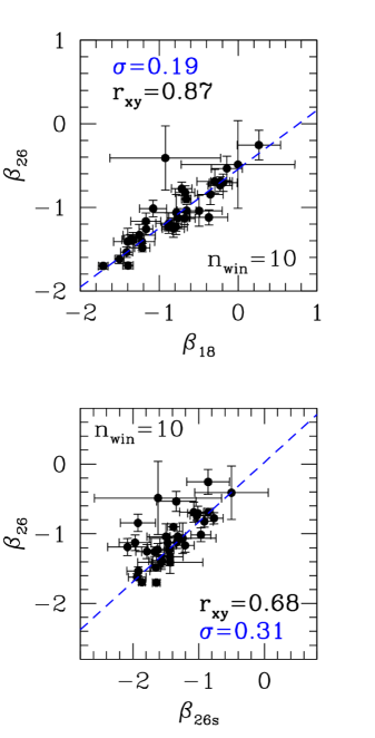
Figure 20: Comparison between $\beta_{26}$, $\beta_{18}$, and $\beta_{26s}$, for the galaxies whose spectrum covers the wavelength range $1250{-}2600{\AA}$. See the text for more details about the definitions of $\beta$. Blue dashed lines indicate the linear fits to the data.

In Section 5.1 we studied the relation between the UV continuum slope and dust attenuation. In galaxies dominated by a young stellar population, the shape of the UV continuum can be fairly accurately approximated by a power law $F_{\lambda}{\varpropto}\lambda^{\beta}$, where $F_{\lambda}$ is the observed flux ($erg\leavevmode\nobreak\ s^{-1}\leavevmode\nobreak\ cm^{-2}\leavevmode\nobreak\ \AA^{-1}$) and $\beta$ is the continuum slope (Calzetti et al. 1994). The wavelength range in which $\beta$ is defined goes from ${\sim}1250{\AA}$ to ${\sim}2600{\AA}$. In this range, Calzetti et al. (1994) defined ten windows to be used to measure the continuum, chosen to avoid the strongest spectral features. For galaxies at $z{\geq}1.6$ $\beta$ was derived through an error-weighted OLS $(Y{\mid}X)$, by fitting the average fluxes in the ten windows defined by Calzetti et al. (1994), in the $log(F_{\lambda})\leavevmode\nobreak\ -\leavevmode\nobreak\ log(\lambda)$ plane. More details about the procedure can be found also in Talia et al. (2012). We define the slope computed using all the ten windows as $\beta_{26}$. Since not all spectra cover the entire $1250{-}2600{\AA}$ range, we define also two shorter versions of $\beta$: $\beta_{18}$, ranging from ${\sim}1250{\AA}$ to ${\sim}1800{\AA}$, and $\beta_{26s}$, ranging from ${\sim}1550{\AA}$ to ${\sim}2600{\AA}$. With respect to the ten original windows, $\beta_{18}$ is measured using the 7 bluer windows (1st to 7th), while $\beta_{26s}$ is measured using the 6 redder ones (5th to 10th).

In Table 5 we indicate the number of galaxies for which each version of the slope could be computed, depending on the wavelength range covered by the spectra.

In Fig. 20 we compare the three definitions of $\beta$ for the galaxies whose spectrum covers the entire wavelength range $1250{-}2600{\AA}$. $\beta_{18}$ is always redder (more positive) than $\beta_{26}$, and the discrepancy increases for increasing value of the slopes (Calzetti 2001).

Table 5: Number of galaxies for which the different definitions of $\beta$ could be computed.

Windows	1st-10th	1st-7th	5th-10th
Tot. no. galaxies	35	33	46
only 24$\mu$m	14	11	17
24$\mu$m and PACS	8	1	11

There is a strong correlation between the two definitions of the slope. In particular, applying an error-weighted linear fit we obtain the following relation ($r_{xy}{\sim}0.9$):

$$\beta_{26}\leavevmode\nobreak\ =\leavevmode\nobreak\ (0.71\pm 0.03)\times\beta_{18}+(-0.54\pm 0.03)$$ (18)

On the other hand, $\beta_{26s}$ is systematically slightly bluer (more negative) than $\beta_{26}$, which is quite intuitive, since $\beta_{18}$ and $\beta_{26s}$ basically sample the two halves of $\beta_{26}$. In this case, a linear fit gives:

$$\beta_{26}\leavevmode\nobreak\ =\leavevmode\nobreak\ (0.86\pm 0.04)\times\beta_{26s}+(0.03\pm 0.06)$$ (19)

with a slightly larger dispersion than in the previous case and no dependence on $\beta_{26}$. The likely explanation of the discrepancy between the three definitions is the presence of a large number of closely spaced Fe absorption lines in the $2300-2800\AA$ range (Leitherer et al. 1999; Calzetti 2001). For each spectrum in the UV sample the appropriate definition of the slope was computed, depending on the wavelength coverage. Then all the $\beta_{18}$ and $\beta_{26s}$ values were scaled to $\beta_{26}$ using Eq. A.1 and Eq. A.2: these homogenised values are the ones that were plotted in Fig. 11 and used to derive the relation given in Sec. 5.1.

As explained in Sec. 5.1, $\beta$ can be derived also from photometry. In the [OII]-sample the available photometry forced us to adopt a short wavelength baseline and we defined $\beta_{phot}$ in the range $\lambda_{rest}{\sim}1500{-}2600\AA$. As we did with the spectroscopic determination of the slope, we used the galaxies in the UV-sample to test the effect of different wavelength baselines also in the computation of the slope from photometry. We found that the values of $\beta_{phot}$ derived using, respectively, the total baseline ($1250-2600\AA$) and a shorter one ($1500-2600\AA$) are broadly consistent with one another, with the short-based values being on average slightly bluer than the long-based ones, though to a lesser extent than in the case of $\beta_{spec}$. Since the short wavelength baseline is available from photometry for the entire galaxy sample, we used directly the values of $\beta_{phot}$ in the range $\lambda_{rest}{\sim}1500-2600\AA$ to obtain the relations presented in Sec. 5.1 and 5.4, without the need to scale them to the total wavelength baseline.