The Lifshitz-Matsubara sum formula for the Casimir pressure between magnetic metallic mirrors
Abstract
We examine the conditions of validity for the Lifshitz-Matsubara sum formula for the Casimir pressure between magnetic metallic plane mirrors. As in the previously studied case of non-magnetic materials (Guérout et al, Phys. Rev. E 90 042125), we recover the usual expression for the lossy model of optical response, but not for the lossless plasma model. We also show that the modes associated with the Foucault currents play a crucial role in the limit of vanishing losses, in contrast to expectations.
pacs:
11.10.Wx, 05.40.-a, 42.50.-p, 78.20.-eI Introduction
The comparison of experimental measurements of Casimir force with theoretical predictions remains a matter of debate Klimchitskaya2006 ; Brevik2006 ; Lambrecht2011 . For experiments performed with mirrors covered by thick layers of gold, optical properties of the metallic mirrors should be deduced from tabulated optical data Lambrecht2000 ; Svetovoy2008 and extrapolated to low frequencies by using the Drude model, with a finite ohmic dissipation rate . However experimental data Decca2007 ; Chang2012 appear to be in better agreement with the so-called plasma model which assumes to vanish, in clear contradiction with the well established fact of a finite static conductivity of gold. This “Casimir puzzle” remains to be solved.
In a previous paper Guerout2014 , we re-examined the conditions of validity of the Lifshitz formulas used to calculate the Casimir pressure. We studied in a very cautious way the positions of the modes of the system in the complex frequency plane, and identified a previously unsuspected problem in the use of the Lifshitz-Matsubara sum formula for the lossless plasma model. As it is usually applied, this formula neglects the contribution of the modes associated with Foucault currents, although the latter tends to a non vanishing limiting value when . While this work did not solve the aforementioned Casimir puzzle, it cured the discontinuity of the calculated Casimir pressure at . It was also interesting from a pure theoretical point of view, as it shed new light on the subtleties of the application of Cauchy’s residue theorem in the context of the calculation of the Casimir pressure.
The Casimir puzzle is not only apparent in experiments performed with gold. It has also been confirmed in recent experiments involving magnetic materials Banishev2012 ; Banishev2013 where, again, experimental measurements appear to agree with predictions based on the non physical lossless plasma model, rather than the much better motivated lossy Drude model. This situation has pushed us to extend our study to include the case of magnetic metallic mirrors. This requires that the mirror’s optical properties be also described by a frequency-dependent permeability , besides the more commonly studied frequency-dependent permittivity . This situation leads to a whole new structure of low frequency modes with a richer phenomenology than in the non-magnetic case.
II Outline
The Casimir pressure between plane mirrors can be calculated equivalently as a Lifshitz integral over real frequencies or as a Lifshitz-Matsubara sum over imaginary frequencies . The two formulations are mathematically related via the application of Cauchy’s residue theorem, and the precise conditions of validity of this equivalence are discussed in Guerout2014 . The optical properties of the mirrors are described by reflection amplitudes for the two polarizations TM and TE, written in terms of permittivity and permeability functions by using Fresnel laws.
We begin with non-magnetic materials, for which the reduced permittivity function is written as
| (1) |
where and are real for all real frequencies . As the dielectric response is causal, the function has an analytic continuation in the upper half-plane which decays fast enough, at least in , so that integration contours can be closed at infinity. It follows, for smooth enough functions, that they obey the Kramers-Kronig relations
| (2) |
for a complex number in the upper half-plane. More generally, causal response functions obey dispersion relations Nussensweig1972 which modify these Kramers-Kronig relations (examples discussed below).
As the response function is real in the time domain, obeys the Schwartz reflection principle along the imaginary axis . For lying on the imaginary axis, one gets the familiar relation
| (3) |
The knowledge of the dissipative part of the permittivity is sufficient for constructing . The latter is deduced from the optical data tabulated over some interval of frequencies from far infrared to ultraviolet in the best scenario, and extrapolated to low and high frequencies Lambrecht2000 ; Svetovoy2008 . In the following, we focus the discussion on the contribution of conduction electrons, dominant at low frequencies. Of course, the contribution of bound electrons has to be included as well in the full analysis.
For metals, the experimental data for have to be extrapolated at low frequencies by using for example the Drude model
| (4) |
is the conductivity, the plasma frequency and the dissipation rate which determines ohmic losses Rakic1998 . The Drude model is the simplest one to match the important fact that metals have a finite static conductivity
| (5) |
and thus to be compatible with Ohm’s law. We note that the function obeys the relation (3) used in many papers as a starting point of the evaluation of Casimir forces. The function appearing in the numerator in the integral (3) is the real part of the conductivity and it is regular everywhere.
The lossless plasma model is obtained by setting in the Drude model
| (6) |
This simplified model can be a fair approximation of the contribution of conduction electrons at large frequencies . However it contains no dissipative part, thus failing to reproduce optical data at low frequencies, and it also misses the fact that metals such as gold have a finite static conductivity (5). The plasma model (6) does not obey the relation (3), as is obvious from the mere fact that vanishes, so that (3) implies , in contradiction with (6).
In more mathematical terms, this defect can be attributed to the fact that has a double pole at the origin or equivalently, that has a simple pole at the origin. A proper application of Cauchy’s theorem then leads to the following expression
| (7) |
where the integral contribution is in fact zero as . In other words, Kramers-Kronig relations do not have any physical content for models which do not include dissipation. For the lossless plasma model, dispersion relations are written with subtractions Nussensweig1972 , which are just modifications of Kramers-Kronig relations.
In our minds, the agreement of measurements with predictions of the plasma model constitutes a problem to be solved, the Casimir puzzle mentioned above. The lossless plasma model, with susceptibility , does not match the optical and electrical properties of gold, and it cannot describe correctly the Casimir pressure between two metallic plates. As already stated, the plasma model can only be considered as an effective model at high frequencies . Considered in this manner, it has to be defined as the limit of the Drude model when
| (8) |
This definition takes care of the problem shown by at by a proper specification of the function there, in the spirit of causality arguments. It gives a susceptibility which differs from , with the difference identified as what is left of dissipation in the vicinity of when . A careful use of the theory of distributions Vladimirov1971 leads to an expression of this difference
| (9) |
The discussions in Guerout2014 prove that predictions based on are then obtained by continuity of those of the Drude model . In contrast, the predictions based on the lossless plasma model , as advocated for example in Mostepanenko2015 , show a discontinuity with those of the Drude model that we will interpret as reflecting the difference (9).
Let us now focus on the extension of the results in Guerout2014 to situations involving magnetic mirrors. We calculate the pressure between two metallic parallel plane mirrors. The mirrors are finite-thickness slabs but we consider the thickness to be large enough so that the mirror’s reflection coefficients are indistinguishable from Fresnel amplitudes. The dielectric properties of mirrors are described by a Drude model at low frequencies. We model the magnetic response by a frequency-dependent permeability as in Banishev2013
| (10) |
This relaxation form is appropriate for describing the spin rotational component of the magnetization. monotonically decreases from to 1 over a characteristic frequency and it has a simple pole at in the complex plane.
The characteristic frequency is by far the lowest frequency in the problem. In Banishev2013 it is argued that lies in a frequency range of the order of – Hz. We may emphasize at this point that this is a further complication for the plasma model scenario. For non magnetic mirrors, the parameter is indeed the lowest frequency in the problem. In contrast, for magnetic materials its physical value is much larger than that of and it makes even less sense to consider . In the following, we will consider different values for , but always stress that its physical value obeys .
In order to specify the other parameters, we will use particular values in the models of permittivity and permeability which match the non-magnetic and magnetic metals used in the experiments, that is to say gold (Au) and nickel (Ni). For gold, we will use eV, meV and ; For nickel, eV, meV, and neV.
The magnetic permeability enters the definition of the Fresnel amplitudes as
| (11) | ||||
In the following we focus on the TE polarization. The Fresnel amplitude when extended to complex frequencies vanishes as at the origin for non-magnetic materials. For magnetic materials, it behaves as at the origin instead. We use notations inspired from our previous work Guerout2014 and write the Casimir pressure calculated using the Lifshitz formula as
| (12) | ||||
where is the distance between the mirrors, the temperature and the polarization. We also recall the Casimir pressure calculated using the Lifshitz-Matsubara sum formula as
| (13) | ||||
where the are the Matsubara frequencies. In this context of the the different models of permittivity used to describe metallic mirrors, we have shown in Guerout2014 that the application of Cauchy’s residue theorem leads to
| (14) | ||||
so that coincide with except if the spectral density contains a Dirac at the origin. Independently of which Lifshitz formula is used, one can use the different susceptibilities introduced before. The susceptibility being a distribution leads to an undefined quantity. On the other hand, we define the Casimir pressures and as the results of the formulas (12) and (13) when using the susceptibility and . Those are well defined quantities and one can study the limit
| (15) |
In Guerout2014 , we have shown that this limit exists and that
| (16) |
Unless otherwise stated, we will work in the following with the quantity for which the two Lifshitz formulas coincide.
We now recall in more detail the main results of our previous work Guerout2014 which uses an elegant extension of the argument principle. In a system of two non-magnetic lossy mirrors the function behaves as at the origin. Therefore, it makes no contribution to the Lifshitz-Matsubara sum formula for the Matsubara frequency (the Lifshitz-Matsubara sum formula picks up a non-vanishing contribution when behaves as at a Matsubara frequency ). At the same time, the modes associated with the Foucault currents lie in an interval , , on the negative imaginary axis of the complex plane. The point is an accumulation point. Thus, there is an infinite number of poles (modes) and zeros in the interval . Nevertheless, one can evaluate the quantity
| (17) |
on a positively-oriented closed contour surrounding the interval to find . This means that possesses two more poles than there are zeros in this interval. As , the interval collapses on the simple zero at the origin leading finally to the function behaving as there. The Lifshitz-Matsubara sum formula now picks up a non-zero contribution from the TE polarization and the Casimir pressure is therefore discontinuous. But as the collapse of the Foucault modes in the interval gives rise to a Dirac contribution in the function .
As mentioned before, this contribution is omitted in the Lifshitz-Matsubara sum formula and must be taken into account explicitly. When this is done it is seen that the contribution from the at the origin exactly cancels out the Matsubara pole contribution there and the Casimir pressure is therefore continuous. We then conclude that the plasma prescription applied to the Lifshitz-Matsubara sum formula fails in taking into account the contribution from the Foucault modes which persists even in the limit of lossless metals. For non-magnetic mirrors, the transverse wavevector is a spectator throughout this process only influencing the value of on the negative imaginary axis. In particular, we have shown that the contribution from the Foucault modes to the Casimir pressure is always repulsive for all for non-magnetic mirrors.
In the following, we study the position of the low frequency modes of the system containing magnetic mirrors as . For mixed magnetic–non-magnetic situations both relaxation rates, e.g. and , go to zero at the same time. An asymptotic regime is achieved when is smaller than the smallest frequency in the problem. In particular, we consider in the following which is not in the physical region.
III The Au-Ni system
We have mentioned that for the Drude permittivity, the point is a pole and an accumulation point. Similarly, for the permeability given by eq. (10) the point is also a pole and an accumulation point. The permeability , extended to the complex plane, gives rise to magnetic modes which lie on the negative imaginary axes in an interval , . Both points and are zeros of . In the limit we have
| (18) | ||||
| (19) |
The Fresnel TE amplitude given by eq. (11) now possesses two zeros on the imaginary axes, which we denote by . The position of those zeros depend on all the parameters of our system. Notably, they depend on . Nevertheless, they satisfy some general properties: one of these zeros always lies on the positive imaginary axis , the other zero always lies on the negative imaginary axis and we have 111 and . Since for this interval must contain at least one zero.. Finally, the function behaves as at the origin so that the TE polarization at does not contribute to the Casimir pressure.

We show in fig. 1 the schematic representation of the low frequency modes of the Au-Ni system, as poles and zeros of the function , in the vicinity of the origin of the complex frequency plane. The modes associated with the Foucault currents are, strictly speaking, both the Foucault modes from the gold and nickel mirrors. As such, the value in the figure is really and . This whole combined structure has as mentioned before. A calculation of on a contour which encloses the interval gives meaning that there is one more pole than there are zeros in this interval.
From our previous work Guerout2014 we know that the interval collapses to the origin as . When dealing with magnetic materials, it turns out that one of the two zeros also collapses to the origin. This leads at the limit to a function behaving as at the origin, as it should. Which of the two zeros collapses to the origin depends on the wavevector : it is easy to show that there is a remarkable value
| (20) |
which corresponds to the condition . Depending on the value of with respect to , one of the two zeros collapses to the origin as
| (21) |
while the other zero tends to a finite value as . Let be the interval supplemented by either or :
| (22) |
The collapse of either set or to the origin is accompanied in the function by the appearance of a Dirac distribution representing the non-vanishing contribution of the Foucault currents at for this particular wavevector . Interestingly, when or respectively, collapses at the origin the function tends towards a positive or negative, respectively, Dirac at the origin. Therefore, when dealing with magnetic materials the total contribution from the Foucault currents at , integrated over all , can in principle be either repulsive or attractive. This is in contrast to what occurs with non-magnetic materials where this contribution was always repulsive Guerout2014 .
IV The Ni-Ni system
The system of two identical magnetic materials inherits many of its analytic properties from the previous Au-Ni system with some slight differences however.
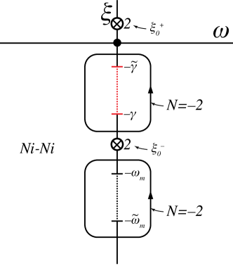
We show in fig. 2 the schematic representation of the low frequency modes of the Ni-Ni system, as poles and zeros of the function , in the vicinity of the origin of the complex frequency plane. First of all, the function now behaves as at the origin so that the TE polarization now contributes to the Lifshitz-Matsubara sum formula at . This is represented by a simple pole which sits at the origin in fig. 2. This simple pole is handled in the usual way by choosing a contour of integration which avoids it (see for instance fig. 1 for the TM polarization of our ref. Guerout2014 ). This leads to the usual contribution to the Casimir pressure at zero frequency which is weighted by a factor . The zeros of the TE Fresnel amplitude and are now double zeros. The set of purely magnetic modes which lie in the interval now correspond to the modes of the two mirrors. As such, a calculation of on a contour enclosing this interval now leads to . The combined sets and have now. When they collapse at the origin, the function still behaves as .
V Total Foucault modes contribution
We show in fig. 3 the contribution of the Foucault modes as a function of the wavevector for the three systems Au-Au, Au-Ni and Ni-Ni. Positive or negative parts, respectively, correspond to repulsive or attractive contributions.

The total contribution to the Casimir pressure is the integral over . This contribution is easily calculated by setting the parameter much smaller than all other frequencies in our problem so that the modes associated with Foucault currents, sitting at frequencies , are well separated from all other modes. Then the quantity
| (23) |
gives the contribution from those modes for a particular wavevector .
As mentioned before, in the case of purely non-magnetic materials (as exemplified by the Au-Au system) the contribution from the Foucault modes are always repulsive for all . On the contrary, in the case of purely magnetic materials the contribution from the Foucault modes is almost always attractive (except for a negligibly small repulsive contribution at low ). In the mixed Au-Ni system, the overall contribution from the Foucault modes is smaller in magnitude. In addition to that, there is now clearly a competition between repulsive and attractive contributions. In the example shown in fig. 3 the total contribution is slightly attractive.
We present in fig. 4 a calculation of the Casimir pressure for Au-Au, Au-Ni and Ni-Ni plane mirrors separated by a distance nm as a function of the relaxation parameter used in the low frequency part of the Drude permittivity .
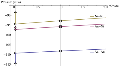
At , the triangles represent obtained using the Lifshitz-Matsubara sum formula whereas the circles represent obtained using the Lifshitz formula. The Foucault modes contribution shown in fig. 3 are directly apparent as the difference between the triangles and the circles.
In the mixed case Au-Ni, it was noted in Banishev2012 that no notable differences was seen in the experimental data and in the calculation between the Drude and the plasma prescription. This fact originates in a coincidental near-degeneracy between the two prescriptions in this case. The puzzle mentioned from the introduction is the fact that experimental data are in very good agreement with the triangles in fig. 4 even though those correspond to inconsistent calculations as we have shown.
In addition to the direct comparison with experiments which measure the Casimir pressure, a recent work Sedighi2015 has shown that whether the calculation is performed using the Drude or plasma models has an impact on the stability of actuation dynamics of microelectromechanical systems.
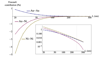
For this reason, we show in fig. 5 the contribution from the Foucault modes as a function of the distance between the plane mirrors. For the Au-Au system, this contribution stays repulsive at all distances. However, for the Au-Ni and Ni-Ni systems, the contribution from Foucault modes stays attractive at all distances. We note that for the mixed Au-Ni system, the Foucault mode contribution which was relatively small at nm (see fig. 4) becomes larger in magnitude than the Au-Au system at shorter distances (see the inset of fig. 5 which shows the contributions, in magnitude, on a log-log scale for the three systems).
VI Conclusion
In this paper, we have confirmed that for both magnetic and non-magnetic metals the contribution from the Foucault modes to the Casimir pressure between plane mirrors reduces to a non-vanishing Dirac at vanishing ohmic losses. We have shown in a previous work Guerout2014 that this contribution is not taken into account when using the so-called plasma prescription in the Lifshitz-Matsubara sum formula which has then to be corrected accordingly. However, contrary to non-magnetic materials, the inclusion of a frequency-dependent permeability can lead, in principle, to either a repulsive or an attractive contribution from those Foucault modes.
In summary, we have extended the careful analysis started in Guerout2014 to magnetic materials. We have been able to prove that there is no discontinuity between the Drude model, which describes the low frequency behavior of metals satisfactorily, and the plasma model, which does not, provided the latter is understood as the limit of the former where the dissipation is taken to zero. Unfortunately, most experiments seem to favor the non-dissipative prescription in which the dissipation is excluded altogether. This problem, called the “Casimir puzzle” in the introduction is seen in experiments involving magnetic materials as well as non magnetic ones and it still remains to be solved.
References
- (1) G.L. Klimchitskaya and V.M. Mostepanenko, Contemp. Phys. 47 131 (2006).
- (2) I. Brevik, S.Å. Ellingsen and K. Milton, New J. Phys. 8 236 (2006).
- (3) A. Lambrecht, A. Canaguier-Durand, R. Guérout and S. Reynaud, in Casimir physics, eds. D.A.R. Dalvit et al, Lecture Notes in Physics 834 (Springer-Verlag, 2011) p.97.
- (4) A. Lambrecht and S. Reynaud, Euro. Phys. J. D 8 309 (2000).
- (5) V.B. Svetovoy, P.J. van Zwol, G. Palasantzas and J.Th.M. De Hosson, Phys. Rev. B 77 035439 (2008).
- (6) R. S. Decca, D. López, E. Fischbach, G. L. Klimchitskaya, D. E. Krause and V. M. Mostepanenko Phys. Rev. D 75, 077101 (2007)
- (7) C.-C. Chang, A. A. Banishev, R. Castillo-Garza et al, Phys. Rev. B 85 165443 (2012).
- (8) R. Guérout, A. Lambrecht, K. A. Milton and S. Reynaud Phys. Rev. E 90, 042125 (2014)
- (9) H. M. Nussenzveig, Causality and Dispersion Relations, (Academic Press New York, 1972).
- (10) A. A. Banishev, C.-C. Chang, G. L. Klimchitskaya, V. M. Mostepanenko and U. Mohideen Phys. Rev. B 85, 195422 (2012)
- (11) A. A. Banishev, G. L. Klimchitskaya, V. M. Mostepanenko and U. Mohideen Phys. Rev. B 88, 155410 (2013)
- (12) A. D. Rakić, A. B. Djurisić, J. M. Elazar and M. L. Majewski Applied Optics 37, 5271 (1998)
- (13) V. S. Vladimirov, Equations of Mathematical Physics, (Decker New York, 1971).
- (14) V.M. Mostepanenko, J. Phys. Condens. Matter 27 214013 (2015).
- (15) M. Sedighi and G. Palasantzas J. App. Phys 117 144901 (2015)