Asynchronous Distributed Semi-Stochastic Gradient Optimization

Abstract

With the recent proliferation of large-scale learning problems, there have been a lot of interest on distributed machine learning algorithms, particularly those that are based on stochastic gradient descent (SGD) and its variants. However, existing algorithms either suffer from slow convergence due to the inherent variance of stochastic gradients, or have a fast linear convergence rate but at the expense of poorer solution quality. In this paper, we combine their merits by proposing a fast distributed asynchronous SGD-based algorithm with variance reduction. A constant learning rate can be used, and it is also guaranteed to converge linearly to the optimal solution. Experiments on the Google Cloud Computing Platform demonstrate that the proposed algorithm outperforms state-of-the-art distributed asynchronous algorithms in terms of both wall clock time and solution quality.

Introduction

With the recent proliferation of big data, learning the parameters in a large machine learning model is a challenging problem. A popular approach is to use stochastic gradient descent (SGD) and its variants (?; ?; ?). However, it can still be difficult to store and process a big data set on one single machine. Thus, there is now growing interest in distributed machine learning algorithms. (?; ?; ?; ?; ?). The data set is partitioned into subsets, assigned to multiple machines, and the optimization problem is solved in a distributed manner.

In general, distributed architectures can be categorized as shared-memory (?) or distributed-memory (?; ?; ?; ?). In this paper, we will focus on the latter, which is more scalable. Usually, one of the machines is the server, while the rest are workers. The workers store the data subsets, perform local computations and send their updates to the server. The server then aggregates the local information, performs the actual update on the model parameter, and sends it back to the workers. Note that workers only need to communicate with the server but not among them. Such a distributed computing model has been commonly used in many recent large-scale machine learning implementations (?; ?; ?; ?).

Often, machines in these systems have to run synchronously (?; ?). In each iteration, information from all workers need to be ready before the server can aggregate the updates. This can be expensive due to communication overhead and random network delay. It also suffers from the straggler problem (?), in which the system can move forward only at the pace of the slowest worker.

To alleviate these problems, asynchronicity is introduced (?; ?; ?; ?; ?). The server is allowed to use only staled (delayed) information from the workers, and thus only needs to wait for a much smaller number of workers in each iteration. Promising theoretical/empirical results have been reported. One prominent example of asynchronous SGD is the downpour SGD (?). Each worker independently reads the parameter from the server, computes the local gradient, and sends it back to the server. The server then immediately updates the parameter using the worker’s gradient information. Using an adaptive learning rate (?), downpour SGD achieves state-of-the-art performance.

However, in order for these algorithms to converge, the learning rate has to decrease not only with the number of iterations (as in standard single-machine SGD algorithms (?)), but also with the maximum delay $\tau$ (i.e., the duration between the time the gradient is computed by the worker and it is used by the server) (?). On the other hand, note that downpour SGD does not constrain $\tau$, but no convergence guarantee is provided.

In practice, a decreasing learning rate leads to slower convergence (?; ?). Recently, ? (?) proposed the delayed proximal gradient method in which the delayed gradient is used to update an analogously delayed model parameter (but not its current one). It is shown that even with a constant learning rate, the algorithm converges linearly to within $\epsilon$ of the optimal solution. However, to achieve a small $\epsilon$, the learning rate needs to be small, which again means slow convergence.

Recently, there has been the flourish development of variance reduction techniques for SGD. Examples include stochastic average gradient (SAG) (?), stochastic variance reduced gradient (SVRG) (?), minimization by incremental surrogate optimization (MISO) (?; ?), SAGA (?), stochastic dual coordinate descent (SDCA) (?), and Proximal SVRG (?). The idea is to use past gradients to progressively reduce the stochastic gradient’s variance, so that a constant learning rate can again be used. When the optimization objective is strongly convex and Lipschitz-smooth, all these variance-reduced SGD algorithms converge linearly to the optimal solution. However, their space requirements are different. In particular, SVRG is advantageous in that it only needs to store the averaged sample gradient, while SAGA and SAG have to store all the samples’ most recent gradients. Recently, ? (?) and ? (?) extended SVRG to the parallel asynchronous setting. Their algorithms are designed for shared-memory multi-core systems, and assume that the data samples are sparse. However, in a distributed computing environment, the samples need to be mini-batched to reduce the communication overhead between workers and server. Even when the samples are sparse, the resultant mini-batch typically is not.

In this paper, we propose a distributed asynchronous SGD-based algorithm with variance reduction, and the data samples can be sparse or dense. The algorithm is easy to implement, highly scalable, uses a constant learning rate, and converges linearly to the optimal solution. A prototype is implemented on the Google Cloud Computing Platform. Experiments on several big data sets from the Pascal Large Scale Learning Challenge and LibSVM archive demonstrate that it outperforms the state-of-the-art.

The rest of the paper is organized as follows. We first introduce related work. Next, we present the proposed distributed asynchronous algorithm. This is then followed by experimental results including comparisons with the state-of-the-art distributed asynchronous algorithms, and the last section gives concluding remarks.

Related Work

Consider the following optimization problem

$$\min_{w}F(w)\equiv\frac{1}{N}\sum_{i=1}^{N}f_{i}(w).$$ (1)

In many machine learning applications, $w\in\mathbb{R}^{d}$ is the model parameter, $N$ is the number of training samples, and each $f_{i}:\mathbb{R}^{d}\rightarrow\mathbb{R}$ is the loss (possibly regularized) due to sample $i$. The following assumptions are commonly made.

Assumption 1

Each $f_{i}$ is $L_{i}$-smooth (?), i.e., $f_{i}(x)\leq f_{i}(y)+\langle\nabla f_{i}(y),x-y\rangle+\frac{L_{i}}{2}\|x-y\|^{2}\;\forall x,y$.

Assumption 2

$F$ is $\mu$-strongly convex (?), i.e., $F(x)\geq F(y)+\langle F(y),x-y\rangle+\frac{\mu}{2}\|x-y\|^{2}\;\forall x,y$.

Delayed Proximal Gradient (DPG)

At iteration $t$ of the DPG (?), a worker uses $w^{t-\tau_{t}}$, the copy of $w$ delayed by $\tau_{t}$ iterations, to compute the stochastic gradient $g^{t-\tau_{t}}=\nabla f_{i}(w^{t-\tau_{t}})$ on a random sample $i$. The delayed gradient is used to update the correspondingly delayed parameter copy $w^{t-\tau_{t}}$ to $\hat{w}^{t-\tau_{t}}=w^{t-\tau_{t}}-\eta g^{t-\tau_{t}}$, where $\eta$ is a constant learning rate. This $\hat{w}^{t-\tau_{t}}$ is then sent to the server, which obtains the new iterate $w^{t+1}$ as a convex combination of the current $w^{t}$ and $\hat{w}^{t-\tau_{t}}$:

$$w^{t+1}=(1-\theta)w^{t}+\theta\hat{w}^{t-\tau_{t}},\;\;\theta\in(0,1].$$ (2)

It can be shown that the $\{w^{t}\}$ sequence converges linearly to the optimal solution $w^{*}$, but only within a tolerance of $\epsilon$, i.e.,

$$\mathbb{E}\left[F(w^{t})-F(w^{*})\right]\leq\rho^{t}(F(w^{0})-F(w^{*}))+\epsilon,$$

for some $\rho<1$ and $\epsilon>0$. The tolerance $\epsilon$ can be reduced by reducing $\eta$, though at the expense of increasing $\rho$ and thus slowing down convergence. Moreover, though the learning rate of DPG is typically larger than that of SGD, the gradient of DPG (i.e., $\hat{w}^{t-\tau_{t}}$) is delayed and slows convergence.

Stochastic Variance Reduced Gradient

The SGD, though simple and scalable, has a slower convergence rate than batch gradient descent (?). As noted in (?), the underlying reason is that the stepsize of SGD has to be decreasing so as to control the gradient’s variance. Recently, by observing that the training set is always finite in practice, a number of techniques have been developed to reduce this variance and thus allows the use of a constant stepsize (?; ?; ?; ?; ?).

In this paper, we focus on one of most popular techniques in this family, namely the stochastic variance reduction gradient (SVRG) (?) (Algorithm 1). It is advantageous in that no extra space is needed for the intermediate gradients or dual variables. The algorithm proceeds in stages. At the beginning of each stage, the gradient $\nabla F(\tilde{w})=\frac{1}{N}\sum_{i=1}^{N}\nabla f_{i}(\tilde{w})$ is computed on the whole data set using a past parameter estimate $\tilde{w}$ (which is updated across stages). For each subsequent iteration $t$ in this stage, the approximate gradient

$$\hat{\nabla}f_{i}(w^{t})=\nabla f_{i}(w^{t})-\nabla f_{i}(\tilde{w})+\nabla F(\tilde{w})$$

is used, where $i$ is a sample randomly selected from $\{1,2,\dots,N\}$. Even with a constant learning rate $\eta$, the (expected) variance of $\hat{\nabla}f(w^{t})$ goes to zero progressively, and the algorithm achieves linear convergence.

Algorithm 1 Stochastic variance reduced gradient (SVRG) (?).

1:  Initialize $\tilde{w}^{0}$;

2:  for $s=1,2,...$ do

3:     $\tilde{w}=\tilde{w}^{s-1}$;

4:     $\nabla F(\tilde{w})=\frac{1}{N}\sum_{i=1}^{N}\nabla f_{i}(\tilde{w})$;

5:     $w^{0}=\tilde{w}$;

6:     for $t=0,1,\dots,m-1$ do

7:        randomly pick $i\in\{1,\dots,N\}$;

8:        $w^{t+1}=w^{t}-\eta\hat{\nabla}f_{i}(w^{t})$;

9:     end for

10:     set $\tilde{w}^{s}=w^{t}$ for a randomly chosen $t\in\{0,\dots,m-1\}$;

11:  end for

In contrast to DPG, SVRG can converge to the optimal solution. However, though SVRG has been extended to the parallel asynchronous setting on shared-memory multi-core systems (?; ?), its use and convergence properties in a distributed asynchronous learning setting remain unexplored.

Proposed Algorithm

In this section, we consider the distributed asynchronous setting, and propose a hybrid of an improved DPG algorithm and SVRG that inherits the advantages of both. Similar to the two algorithms, it also uses a constant learning rate (which is typically larger than the one used by SGD), but with guaranteed linear convergence to the optimal solution.

Update using Delayed Gradient

We replace the SVRG update (line 8 in Algorithm 1) by

$$w^{t+1}=(1-\theta)v^{t}+\theta\bar{w}^{t-\tau_{t}},$$ (3)

where

$$v^{t}=w^{t}-\eta\hat{\nabla}f_{i}(w^{t-\tau_{t}})$$

and

$$\bar{w}^{t-\tau_{t}}=w^{t-\tau_{t}}-\eta\hat{\nabla}f_{i}(w^{t-\tau_{t}}).$$ (4)

Obviously, when $\tau_{t}=0$, (3) reduces to standard SVRG. Note that both the parameter and gradient in $\bar{w}^{t-\tau_{t}}$ are for the same iteration ($t-\tau_{t}$), while $v^{t}$ is noisy as the gradient is delayed (by $\tau_{t}$). This delayed gradient cannot be too old. Thus, similar to (?), we impose the bounded delay condition that $\tau_{t}\leq\tau$ for some $\tau>0$. This $\tau$ parameter determines the maximum duration between the time the gradient is computed and till it is used. A larger $\tau$ allows more asynchronicity, but also adds noise to the gradient and thus may slow convergence.

Update (3) is similar to (2) in DPG, but with two important differences. First, the gradient $\nabla f_{i}(w^{t-\tau_{t}})$ in DPG is replaced by its variance-reduced counterpart $\hat{\nabla}f_{i}(w^{t-\tau_{t}})$. As will be seen, this allows convergence to the optimal solution using a constant learning rate. The second difference is that the delayed gradient $\hat{\nabla}f_{i}(w^{t-\tau_{t}})$ is used not only on the past iterate $w^{t-\tau_{t}}$, but also on the current iterate $w^{t}$. This can potentially yield faster progress, as is most apparent when $\theta=0$. In this special case, DPG reduces to $w^{t+1}=w^{t}$, and makes no progress; while (3) reduces to the asynchronous SVRG update in (?).

Mini-Batch

In a distributed algorithm, communication overhead is incurred when a worker pulls parameters from the server or pushes update to it. In a distributed SGD-based algorithm, the communication cost is proportional to the number of gradient evaluations made by the workers. Similar to the other SGD-based distributed algorithms (?; ?; ?), this cost can be reduced by the use of a mini-batch. Instead of pulling parameters from the server after every sample, the worker pulls only after processing each mini-batch of size $B$.

Distributed Implementation

There is a scheduler, a server and $P$ workers. The server keeps a clock (denoted by an integer $t$), the most updated copy of parameter $w$, a past parameter estimate $\tilde{w}$ and the corresponding full gradient $\nabla F(\tilde{w})$ evaluated on the whole training set $\mathcal{D}$ (with $N$ samples). We divide $\mathcal{D}$ into $P$ disjoint subsets $\mathcal{D}_{1},\mathcal{D}_{2},\dots,\mathcal{D}_{P}$, where $\mathcal{D}_{p}$ is owned by worker $p$. The number of samples in $\mathcal{D}_{p}$ is denoted $n_{p}$. Each worker $p$ also keeps a local copy $\tilde{w}_{p}$ of $\tilde{w}$.

In the following, a task refers to an event timestamped by the scheduler. It can be issued by the scheduler or a worker, and received by either the server or workers. Each worker can only process one task at a time. There are two types of tasks, update task and evaluation task, and will be discussed in more detail in the sequel. A worker may pull the parameter from the server by sending a request, which carries the type and timestamp of the task being run by the worker.

Scheduler

The scheduler (Algorithm 2) runs in stages. In each stage, it first issues $m$ update tasks to the workers, where $m$ is usually a multiple of $\lceil N/B\rceil$ as in SVRG. After spawning enough tasks, the server measures the progress by issuing an evaluation task to the server and all workers. As will be seen, the server ensures that evaluation is carried out only after all update tasks for the current stage have finished. If the stopping condition is met, the scheduler informs the server and all workers by issuing a STOP command; otherwise, it moves to the next stage and sends more update tasks.

Algorithm 2 Scheduler.

1:  for $s=1,\dots,S$ do

2:     for $k=1,\dots,m$ do

3:        pick worker $p$ with probability $\frac{n_{p}}{N}$;

4:        issue an update task to the worker with timestamp $t=(s-1)m+k$;

5:     end for

6:     issue an evaluation task (with timestamp $t=sm+1$) to workers and server;

7:     wait and collect progress information from workers;

8:     if progress meets stopping condition then

9:        issue a STOP command to the workers and server;

10:     end if

11:  end for

Worker

At stage $s$, when worker $p$ receives an update task with timestamp $t$, it sends a parameter pull request to the server. This request will not be responded by the server until it finishes all tasks with timestamps before $t-\tau$.

Let $\hat{w}_{p,t}$ be the parameter value pulled. Worker $p$ selects a mini-batch $\mathcal{B}^{t}\subset\mathcal{D}_{p}$ (of size $B$) randomly from its local data set. Analogous to $\bar{w}^{t-\tau_{t}}$ in (4), it computes

$$\bar{w}_{p,t}=\hat{w}_{p,t}-\eta\Delta w_{p,t},$$ (5)

where $\Delta w_{p,t}$ is the mini-batch gradient evaluated at $\hat{w}_{p,t}$. An update task is then issued to push $\bar{w}_{p,t}$ and $\Delta w_{p,t}$ to the server.

When a worker receives an evaluation task, it again sends a parameter pull request to the server. As will be seen in the following section, the pulled $\hat{w}_{p,t}$ will always be the latest $w$ kept by the server in the current stage. Hence, the $\hat{w}_{p,t}$’s pulled by all workers are the same. Worker $p$ then updates $\tilde{w}_{p}$ as $\tilde{w}_{p}=\hat{w}_{p,t}$, computes and pushes the corresponding gradient

$$\nabla F_{p}(\tilde{w}_{p})=\frac{1}{n_{p}}\sum_{i\in\mathcal{D}_{p}}\nabla f_{i}(\tilde{w}_{p})$$

to the server. To inform the scheduler of its progress, worker $p$ also computes its contribution to the optimization objective $\sum_{i\in\mathcal{D}_{p}}f_{i}(\tilde{w}_{p})$ and pushes it to the scheduler. The whole worker procedure is shown in Algorithm 3.

Algorithm 3 Worker $p$ receiving an update/evaluation task $t$ at stage $s$.

1:  send a parameter pull request to the server;

2:  wait for response from the server;

3:  if task $t$ is an update task then

4:     pick a mini-batch subset $\mathcal{B}^{t}$ randomly from the local data set;

5:     compute mini-batch gradient $\Delta w_{p,t}$ and $\bar{w}_{p,t}$ using (5), and push them to the server as an update task;

6:  else

7:     set $\tilde{w}_{p}=\hat{w}_{p,t}$; {task $t$ is an evaluation task}

8:     push the local subset gradient $\nabla F_{p}(\tilde{w}_{p})$ to the server as an update task;

9:     push the local objective value to the scheduler;

10:  end if

Server

There are two threads running on the server. One is a daemon thread that responds to parameter pull requests from workers (Algorithm 4); and the other is a computing thread for handling update tasks from workers and evaluation tasks from the scheduler (Algorithm 5).

When the daemon thread receives a parameter pull request, it reads the type and timestamp $t$ within. If the request is from a worker running an update task, it checks whether all update tasks before $t-\tau$ have finished. If not, the request remains in the buffer; otherwise, it pushes its $w$ value to the requesting worker. Thus, this controls the allowed asynchronicity. On the other hand, if the request is from a worker executing an evaluation task, the daemon thread does not push $w$ to the workers until all update tasks before $t$ have finished. This ensures that the $w$ pulled by the worker is the most up-to-date for the current stage.

Algorithm 4 Daemon thread of the server.

1:  repeat

2:     if pull request buffer is not empty then

3:        for each request with timestamp $t$ in the buffer do

4:           if request is triggered by an update task then

5:              if all update tasks before $t-\tau$ have finished then

6:                 push $w$ to the requesting worker;

7:                 remove request from buffer;

8:              end if

9:           else

10:              if all update tasks before $t$ have finished then

11:                 push $w$ to the requesting worker;

12:                 remove request from buffer;

13:              end if

14:           end if

15:        end for

16:     else

17:        sleep for a while;

18:     end if

19:  until STOP command is received.

When the computing thread receives an update task (with timestamp $t$) from worker $p$, the $\bar{w}_{p,t}$ and $\Delta w_{p,t}$ contained inside are read. Analogous to (3), the server updates $w$ as

$$w =(1-\theta)(w-\eta\Delta w_{p,t})+\theta\bar{w}_{p,t},$$ (6)

and marks this task as finished. During the update, the computing thread locks $w$ so that the daemon thread cannot access until the update is finished.

When the server receives an evaluation task, it synchronizes all workers, and sets $\tilde{w}=w$. As all $\tilde{w}_{p}$’s are the same and equal to $\tilde{w}$, one can simply aggregate the local gradients to obtain $\nabla F(\tilde{w})=\sum_{p=1}^{P}q_{p}\nabla F_{p}(\tilde{w}_{p})$, where $q_{p}=\frac{n_{p}}{N}$. The server then broadcasts $\nabla F(\tilde{w})$ to all workers.

Algorithm 5 Computing thread of the server.

1:  repeat

2:     wait for tasks;

3:     if an update task received then

4:        update $w$ using (6), and mark this task as finished;

5:     else

6:        wait for all update tasks to finish;

7:        set $\tilde{w}=w$;

8:        collect local full gradients from workers and update $\nabla F(\tilde{w})$;

9:        broadcast $\nabla F(\tilde{w})$ to all workers;

10:     end if

11:  until STOP command is received.

Discussion

Two state-of-the-art distributed asynchronous SGD algorithms are the downpour SGD (?) and Petuum SGD (?; ?). Downpour SGD does not impose the bounded delay condition (essentially, $\tau=\infty$), while Petuum SGD does. Note that there is a subtle difference in the bounded delay condition of the proposed algorithm and that of Petuum SGD. In Petuum SGD, the amount of staleness is measured between workers, namely that the slowest and fastest workers must be less than $s$ timesteps apart (where $s$ is the staleness parameter). Consequently, the delay in the gradient is always a multiple of $P$ and is upper-bounded by $sP$. On the other hand, in the proposed algorithm, the bounded delay condition is imposed on the update tasks. It can be easily seen that $\tau$ is also the maximum delay in the gradient. Thus, $\tau$ can be any number which is not necessarily a multiple of $P$.

Convergence Analysis

For simplicity of analysis, we assume that the mini-batch size is one. Let $\tilde{w}^{S}$ be the $w$ stored in the server at the end of stage $S$ (step 7 in Algorithm 5). The following Theorem shows linear convergence of the proposed algorithm. It is the first such result for distributed asynchronous SGD-based algorithms with constant learning rate.

Theorem 3

Suppose that problem (1) satisfies Assumption 1 and 2. Let $L=\max\{L_{i}\}_{i=1}^{N}$, and $\gamma=\left(1-2\eta(\mu-\frac{\eta L^{2}}{\theta})\right)^{\frac{m}{1+\tau}}+\frac{\eta L^{2}}{\theta\mu-\eta L^{2}}$. With $\eta\in(0,\frac{\mu\theta}{2L^{2}})$ and $m$ sufficiently large such that $\gamma<1$. Assume that the scheduler has been run for $S$ stages, we obtain the following linear rate:

$$\mathbb{E}[F(\tilde{w}^{S})-F(w^{*})]\leq\;\;\gamma^{S}[F(\tilde{w}^{0})-F(w^{*})].$$

As $L>\mu$, it is easy to see that $1-2\eta(\mu-\frac{\eta L^{2}}{\theta})$ and $\frac{\eta L^{2}}{\theta\mu-\eta L^{2}}$ are both smaller than 1. Thus, $\gamma<1$ can be guaranteed for a sufficiently large $m$. Moreover, as $F$ is strongly convex, the following Corollary shows that $\tilde{w}^{S}$ also converges to $w^{*}$. In contrast, DPG only converges to within a tolerance of $\epsilon$.

Corollary 4

$\mathbb{E}\|\tilde{w}^{S}-w^{*}\|^{2}\leq 2\gamma^{S}[F(\tilde{w}^{0})-F(w^{*})]/\mu$.

When $\tau<P$, the server can serve at most $\tau$ workers simultaneously. For maximum parallelism, $\tau$ should increase with $P$. However, $\gamma$ also increases with $\tau$. Thus, a larger $m$ and/or $S$ may be needed to achieve the same solution quality.

Similar to DPG, our learning rate does not depend on the delay $\tau$ and the number of workers $P$. This learning rate can be significantly larger than the one in Pentuum SGD (?), which has to be decayed and is proportional to $\mathcal{O}(1/\sqrt{P})$. Thus, the proposed algorithm can be much faster, as will be confirmed in the experiments. While our bound may be loose due to the use of worst-case analysis, linear convergence is always guaranteed for any $\theta\in(0,1]$.

Experiments

In this section, we consider the $K$-class logistic regression problem:

$$\min_{\{w_{k}\}_{k=1}^{K}}\frac{1}{N}\sum_{i=1}^{N}\sum_{k=1}^{K}-I(y_{i}=k)\log\left(\frac{\exp(w_{k}^{T}x_{i})}{\sum_{j=1}^{K}\exp(w_{j}^{T}x_{i})}\right),$$

where $\{(x_{i},y_{i})\}_{i=1}^{N}$ are the training samples, $w_{k}$ is the parameter vector of class $k$, and $I(\cdot)$ is the indicator function which returns 1 when the argument holds, and 0 otherwise. Experiments are performed on the Mnist8m and DNA data sets (Table 1) from the LibSVM archive and Pascal Large Scale Learning Challenge.

	#samples	#features	#classes
Mnist8m	8,100,000	784	10
DNA	50,000,000	800	2

Table 1: Summary of the data sets used.

Using the Google Cloud Computing Platform, we set up a cluster with 18 computing nodes. Each node is a google cloud n1-highmem-8 instance with eight cores and 52GB memory. Each scheduler/server takes one instance, while each worker takes a core. Thus, we have a maximum of 128 workers. The system is implemented in C++, with the ZeroMQ package for communication.

Comparison with the State-of-the-Art

In this section, the following distributed asynchronous algorithms are compared:

• Downpour SGD (“downpour-sgd”) (?), with the adaptive learning rate in Adagrad (?);

• Petuum SGD (?) (“petuum-sgd”), the state-of-the-art implementation of asynchronous SGD. The learning rate is reduced by a fixed factor 0.95 at the end of each epoch. The staleness $s$ is set to $2$, and so the delay in the gradient is bounded by 2$P$.

• DPG (?) (“dpg”);

• A variant of DPG (“vr-dpg“), in which the gradient in update (2) is replaced by its variance-reduced version;

• The proposed “distributed variance-reduced stochastic gradient decent” (distr-vr-sgd) algorithm.

• A special case of distr-vr-sgd, with $\theta=0$ (denoted “distr-svrg“). This reduces to the asynchronous SVRG algorithm in (?).

We use 128 workers. To maximize parallelism, we fix $\tau$ to 128. The Petuum SGD code is downloaded from http://petuum.github.io/, while the other asynchronous algorithms are implemented in C++ by reusing most of our system’s codes. Preliminary studies show that synchronous SVRG is much slower and so is not included for comparison. For distr-vr-sgd and distr-svrg, the number of stages is $S=50$, and the number of iterations in each stage is $m=\lceil N/B\rceil$, where $B$ is about $10\%$ of each worker’s local data set size. For fair comparison, the other algorithms are run for $mS$ iterations. All other parameters are tuned by a validation set, which is $1\%$ of the data set.

Figure 1 shows convergence of the objective w.r.t. wall clock time. As can be seen, distr-vr-sgd outperforms all the other algorithms. Moreover, unlike dpg, it can converge to the optimal solution and attains a much smaller objective value. Note that distr-svrg is slow. Since $\tau=128$, the delayed gradient can be noisy, and the learning rate used by distr-svrg (as determined by the validation set) is small ($10^{-6}$ vs $10^{-3}$ in distr-vr-sgd). On the DNA data set, distr-svrg is even slower than petuum-sgd and downpour-sgd (which use adaptive/decaying learning rates). The vr-dpg, which uses variance-reduced gradient, is always faster than dpg. Moreover, distr-vr-sgd is faster than vr-sgd, showing that replacing $w^{t}$ in (2) by $v^{t}$ in (3) is useful.

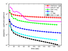
(a) Mnist8m.

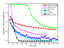
(b) DNA.

Figure 1: Objective vs time (in sec).

Varying the Number of Workers

In this experiment, we run distr-vr-sgd with varying number of workers (16, 32, 64 and 128) until a target objective value is met. Figure 2 shows convergence of the objective with time. On the Mnist8m data set, using 128 workers is about 3 times faster than using 16 workers. On the DNA data set, the speedup is about 6 times.

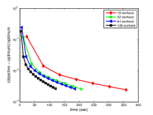
(a) Mnist8m.

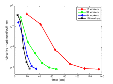
(b) DNA.

Figure 2: Objective vs time (in sec), with different numbers of workers.

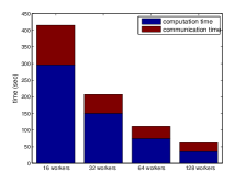
(a) Mnist8m.

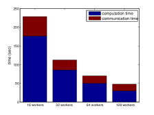
(b) DNA.

Figure 3: Breakdown into computation time and communication time, with different numbers of workers.

Note that the most expensive step in the algorithm is on gradient evaluations (the scheduler and server operations are simple). Recall that each stage has $m$ iterations, and each iteration involvs $O(B)$ gradient evaluations. At the end of each stage, an additional $O(N)$ gradients are evaluated to obtain the full gradient and monitor the progress. Hence, each worker spends $\mathcal{O}((mB+N)/P)$ time on computation. The computation time thus decreases linearly with $P$, as can be seen from the breakdown of total wall clock time into computation time and communication time in Figure 3.

Moreover, having more workers means more tasks/data can be sent among the server and workers simultaneously, reducing the communication time. On the other hand, as synchronization is required among all workers at the end of each stage, having more workers increases the communication overhead. Hence, as can be seen from Figure 3, the communication time first decreases with the number of workers, but then increases as the communication cost in the synchronization step starts to dominate.

Effect of $\tau$

In this experiment, we use 128 workers. Figure 4 shows the time for distr-vr-sgd to finish $mS$ tasks (where $S=50$ and $m=\lceil N/B\rceil$) when $\tau$ is varied from 10 to 200. As can be seen, with increasing $\tau$, higher asynchronicity is allowed, and the communication cost is reduced significantly.

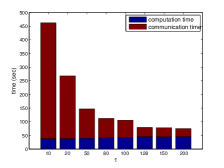
(a) Mnist8m.

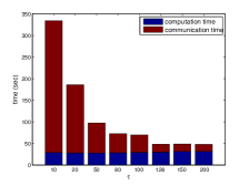
(b) DNA.

Figure 4: Breakdown of the total time into computation time and communication time, with different $\tau$’s.

Conclusion

Existing distributed asynchronous SGD algorithms often rely on a decaying learning rate, and thus suffer from a sublinear convergence rate. On the other hand, the recent delayed proximal gradient algorithm uses a constant learning rate and has linear convergence rate, but can only converge to within a neighborhood of the optimal solution. In this paper, we proposed a novel distributed asynchronous SGD algorithm by integrating the merits of the stochastic variance reduced gradient algorithm and delayed proximal gradient algorithm. Using a constant learning rate, it still guarantees convergence to the optimal solution at a fast linear rate. A prototype system is implemented and run on the Google cloud platform. Experimental results show that the proposed algorithm can reduce the communication cost significantly with the use of asynchronicity. Moreover, it converges much faster and yields more accurate solutions than the state-of-the-art distributed asynchronous SGD algorithms.

References

- [Agarwal and Duchi 2011] Agarwal, A., and Duchi, J. 2011. Distributed delayed stochastic optimization. In Advances in Neural Information Processing Systems 24.
- [Albrecht et al. 2006] Albrecht, J.; Tuttle, C.; Snoeren, A.; and Vahdat, A. 2006. Loose synchronization for large-scale networked systems. In Proceedings of the USENIX Annual Technical Conference, 301–314.
- [Bottou 2010] Bottou, L. 2010. Large-scale machine learning with stochastic gradient descent. In Proceedings of the International Conference on Computational Statistics. 177–186.
- [Boyd et al. 2011] Boyd, S.; Parikh, N.; Chu, E.; Peleato, B.; and Eckstein, J. 2011. Distributed optimization and statistical learning via the alternating direction method of multipliers. Foundations and Trends in Machine Learning 3(1):1–122.
- [Dai et al. 2013] Dai, W.; Wei, J.; Zheng, X.; Kim, J. K.; Lee, S.; Yin, J.; Ho, Q.; and Xing, E. P. 2013. Petuum: A framework for iterative-convergent distributed ML. Technical Report arXiv:1312.7651.
- [Dean et al. 2012] Dean, J.; Corrado, G.; Monga, R.; Chen, K.; Devin, M.; Mao, M.; Senior, A.; Tucker, P.; Yang, K.; Le, Q. V.; et al. 2012. Large scale distributed deep networks. In Advances in Neural Information Processing Systems, 1223–1231.
- [Defazio, Bach, and Lacoste-Julien 2014] Defazio, A.; Bach, F.; and Lacoste-Julien, S. 2014. SAGA: A fast incremental gradient method with support for non-strongly convex composite objectives. In Advances in Neural Information Processing Systems, 1646–1654.
- [Duchi, Hazan, and Singer 2011] Duchi, J.; Hazan, E.; and Singer, Y. 2011. Adaptive subgradient methods for online learning and stochastic optimization. Journal of Machine Learning Research 12:2121–2159.
- [Feyzmahdavian, Aytekin, and Johansson 2014] Feyzmahdavian, H. R.; Aytekin, A.; and Johansson, M. 2014. A delayed proximal gradient method with linear convergence rate. In Proceedings of the International Workshop on Machine Learning for Signal Processing, 1–6.
- [Gimpel, Das, and Smith 2010] Gimpel, K.; Das, D.; and Smith, N. A. 2010. Distributed asynchronous online learning for natural language processing. In Proceedings of the 14th Conference on Computational Natural Language Learning, 213–222.
- [Ho et al. 2013] Ho, Q.; Cipar, J.; Cui, H.; Lee, S.; Kim, J.; Gibbons, P.; Gibson, G.; Ganger, G.; and Xing, E. 2013. More effective distributed ML via a stale synchronous parallel parameter server. In Advances in Neural Information Processing Systems 26, 1223–1231.
- [Johnson and Zhang 2013] Johnson, R., and Zhang, T. 2013. Accelerating stochastic gradient descent using predictive variance reduction. In Advances in Neural Information Processing Systems, 315–323.
- [Li et al. 2014] Li, M.; Andersen, D. G.; Smola, A. J.; and Yu, K. 2014. Communication efficient distributed machine learning with the parameter server. In Advances in Neural Information Processing Systems, 19–27.
- [Mairal 2013] Mairal, J. 2013. Optimization with first-order surrogate functions. In Proceedings of the 30th International Conference on Machine Learning.
- [Mairal 2015] Mairal, J. 2015. Incremental majorization-minimization optimization with application to large-scale machine learning. Technical Report arXiv:1402.4419.
- [Mania et al. 2015] Mania, H.; Pan, X.; Papailiopoulos, D.; Recht, B.; Ramchandran, K.; and Jordan, M. I. 2015. Perturbed iterate analysis for asynchronous stochastic optimization. Technical Report arXiv:1507.06970.
- [Nesterov 2004] Nesterov, Y. 2004. Introductory Lectures on Convex Optimization, volume 87. Springer Science & Business Media.
- [Niu et al. 2011] Niu, F.; Recht, B.; Ré, C.; and Wright, S. 2011. Hogwild!: A lock-free approach to parallelizing stochastic gradient descent. In Advances in Neural Information Processing Systems 24.
- [Reddi et al. 2015] Reddi, S. J.; Hefny, A.; Sra, S.; Póczos, B.; and Smola, A. 2015. On variance reduction in stochastic gradient descent and its asynchronous variants. Technical Report arXiv:1506.06840.
- [Roux, Schmidt, and Bach 2012] Roux, N. L.; Schmidt, M.; and Bach, F. R. 2012. A stochastic gradient method with an exponential convergence rate for finite training sets. In Advances in Neural Information Processing Systems, 2663–2671.
- [Shalev-Shwartz and Zhang 2013] Shalev-Shwartz, S., and Zhang, T. 2013. Stochastic dual coordinate ascent methods for regularized loss. Journal of Machine Learning Research 14(1):567–599.
- [Shamir, Srebro, and Zhang 2014] Shamir, O.; Srebro, N.; and Zhang, T. 2014. Communication-efficient distributed optimization using an approximate Newton-type method. In Proceedings of the 31st International Conference on Machine Learning, 1000–1008.
- [Xiao and Zhang 2014] Xiao, L., and Zhang, T. 2014. A proximal stochastic gradient method with progressive variance reduction. SIAM Journal on Optimization 24(4):2057–2075.
- [Zhang and Kwok 2014] Zhang, R., and Kwok, J. 2014. Asynchronous distributed ADMM for consensus optimization. In Proceedings of the 31st International Conference on Machine Learning, 1701–1709.