Electron correlation effects in enhanced-ionization of molecules: A time-dependent generalized-active-space configuration-interaction study

Abstract

We numerically study models of $\mathrm{H}_{2}$ and $\mathrm{LiH}$ molecules, aligned collinearly with the linear polarization of the external field, to elucidate the possible role of correlation in the enhanced-ionization phenomena. Correlation is considered at different levels of approximation with the time-dependent generalized-active-space configuration-interaction method. The results of our studies show that enhanced ionization occurs in multielectron molecules, that correlation is important and they also demonstrate significant deviations between the results of the single-active-electron approximation and more accurate configuration-interaction methods. With the inclusion of correlation we show strong carrier-envelope-phase effects in the enhanced ionization of the asymmetric heteronuclear $\mathrm{LiH}$-like molecule. The correlated calculation shows an intriguing feature of cross-over in enhanced ionization with two carrier-envelope-phases at critical inter-nuclear separation.

I Introduction

When a diatomic molecule is exposed to ultra-short laser pulses, the ionization yield is enhanced at certain critical inter-nuclear distances. This phenomenon is known as enhanced ionization (EI) and has been observed both experimentally Constant et al. (1996); Pavičić et al. (2005); Ben-Itzhak et al. (2008); Bocharova et al. (2011); Wu et al. (2012); Lai and Guo (2014); Xu et al. (2015) and discussed theoretically  Seideman et al. (1995); Zuo and Bandrauk (1995); Chelkowski and Bandrauk (1995); Mulyukov et al. (1996); Plummer and McCann (1996); Villeneuve et al. (1996) (see Ref. Bandrauk and Légaré (2012) for a review on EI in molecules). The main interesting feature that distinguishes ionization of a diatomic molecule from ionization of an atom is the double-well structure of the potential. At the equilibrium inter-nuclear separation, the molecular potential is dominated by the Coulombic monopole and in this sense it is similar to the atomic potential. As the inter-nuclear separation ${R}$ increases, the internal barrier between the two wells broadens. In the presence of a strong electric field the diatomic potential is distorted and the potential changes drastically. Since the barrier height in one of the well reduces, the electron can directly tunnel to the continuum and this effect enhances the ionization probability at certain critical inter-nuclear distance. For one-electron systems, the localization of the wave function in the upper well of the effective potential formed by the molecular potential and the external field is a key mechanism as explained in Ref. Seideman et al. (1995). It was shown earlier that electron localization in the presence of a strong field is an often encountered phenomenon Grossmann et al. (1991); Bavli and Metiu (1992). The probability of localization in one of the wells depends on the laser intensity and frequency as well as on the phase Bavli and Metiu (1992). It is also important to emphasize that the localization of the electronic wave packet depends on the preparation of the initial state. In Ref. Zuo and Bandrauk (1995) a different mechanism for EI was proposed. In that work EI is seen as the results of the creation of a pair of charge-resonant (CR) states which strongly couples to the external field at the critical inter-nuclear distance. Along with the creation of CR states the potential experienced by the electron is also changed in the presence of the strong field. This is also known as charge-resonance-enhanced-ionization (CREI) of diatomic molecules. A one-dimensional model of $\mathrm{H}_{2}$ was studied in Ref. Yu et al. (1996) and a full three-dimensional calculation of $\mathrm{H}_{2}$ was presented recently Dehghanian et al. (2010). For a one-electron system like $\mathrm{H}_{2}^{+}$, it has been widely discussed from which well of the diatomic potential the electron will escape. In Ref. Mulyukov et al. (1996), it is argued that the ionization can occur by resonant transition to an excited state supported by the lower well. Using $\mathrm{H}_{2}$, it is also argued that the EI in diatomic molecules occurs due to level crossings between the ground state and that of the excited states which dissociate into ionic fragments Saenz (2000, 2002). The EI in more complex, e.g., asymmetric molecules was studied in Ref. Kamta and Bandrauk (2005, 2007); Dehghanian et al. (2013). Experimentally the EI was found in molecular iodine Constant et al. (1996), and in molecular ions Pavičić et al. (2005); Ben-Itzhak et al. (2008). The EI in ${\mathrm{CO}}_{2}$ was experimentally studied in Ref. Bocharova et al. (2011), and in Ref.  Wu et al. (2012) the tunneling site of the electron that takes part in the EI of molecules was experimentally probed. Recent experiments directly detected EI in $\mathrm{CO}$ and $\mathrm{N}_{2}$ Lai and Guo (2014) and demonstrated a two peak structure of EI in $\mathrm{H}_{2}^{+}$ Xu et al. (2015).

Solving the time-dependent Schrödinger equation (TDSE) directly in the presence of a strong external field is possible only for atoms and molecules with one or two electrons. Most of the previous calculations therefore use the single-active-electron (SAE) approximation. They may, therefore, neglect some important features which may arise due to electron correlation. The purpose of this work is to elucidate EI further by investigating in a systematic manner the role of electron correlation on this mechanism. Several time-dependent many-body methods have been developed to take into account electron correlation as accurately as possible. The time-dependent $R$-matrix approach  van der Hart et al. (2007); Lysaght et al. (2008, 2009); van der Hart (2014), the time-dependent configuration-interaction singles (TDCIS) approximation Krause et al. (2005); Rohringer et al. (2006); Greenman et al. (2010); Karamatskou et al. (2014), the multiconfigurational time-dependent Hartree-Fock method Kato and Kono (2004); Nest et al. (2005); Caillat et al. (2005); Hochstuhl et al. (2010); Haxton et al. (2011, 2012); Hochstuhl et al. (2014) and its generalizations Miyagi and Madsen (2013); Sato and Ishikawa (2013); Miyagi and Madsen (2014a, b); Sato and Ishikawa (2015) have been applied to processes involving laser-matter interactions. The time-dependent restricted-active-space configuration-interaction (TD-RASCI) method Hochstuhl and Bonitz (2012), and time-dependent generalized-active-space (TD-GASCI) configuration-interaction method Bauch et al. (2014); Larsson et al. (2015) systematically take into account the electron correlation through a configuration-interaction expansion within a mixed-basis set approach with localized and grid-based orbitals to allow for an accurate description of both, the bound and continuum states. This method includes the limits of full CI, the SAE and the CIS approximations. The TD-GASCI method has been used to calculate the photoelectron spectra of one-dimensional two and four electron atoms and molecules Bauch et al. (2014) and the TD-RASCI method to calculate photoionization cross sections of beryllium and neon Hochstuhl and Bonitz (2012). In the present work, we use the TD-GASCI method to study correlation phenomena in EI of model molecules. First, we consider a model of ${\mathrm{H}}_{2}$. In this homonuclear system we study the convergence of the TD-GASCI method by comparing it with fully correlated (“exact”) TDSE calculations. To study the correlation trend we use linearly polarized laser fields polarized along the inter-nuclear axis within the fixed-nuclei approximation. Further we consider a model of ${\mathrm{LiH}}$ and report on EI phenomena within four electron molecules. In this asymmetric system we study the correlation effects in EI and in addition the sensitivity to the relative orientation between the molecule and the dominant half-cycle of the short pulse as controlled by the carrier-envelope-phase (CEP).

The paper is organized as follows. In Sec. II, we briefly present the TD-GASCI method and the special basis set used. In Sec. III, we use the TD-GASCI method to calculate the ionization yield as a function of inter-nuclear distance to study the EI phenomena. We demonstrate the accuracy of the TD-GAS-CI results of the $\mathrm{H}_{2}$ model by comparison with TDSE results. Further we consider calculations for the $\mathrm{LiH}$ model with different GAS partitions corresponding to accounting for electron correlation at different levels of approximation. In Sec. IV, we summarize our work and conclude.

II Theory

Here we briefly recall the TD-GASCI methodology Bauch et al. (2014). To ease notation we consider a diatomic molecule with nuclei at $\pm{R/2}$ and charges $Z_{1}$ and $Z_{2}$, respectively. The TDSE for $N_{el}$ -electrons with fixed nuclei then reads (we use atomic units throughout this work)

$$i\frac{\partial}{\partial t}|\Psi(t)\rangle=H(t)|\Psi(t)\rangle\;.$$ (1)

The time-dependent Hamiltonian is given by

$$H(t)=\sum_{i=1}^{N_{el}}{h}_{i}(t)+\sum_{i<j}^{N_{el}}w_{ij}\;,$$ (2)

with the one-body part of electron $i$ given by

$${h}_{i}(t)=-\frac{1}{2}\nabla_{i}^{2}-\frac{Z_{1}}{|\bm{r}_{i}-\frac{\bm{R}}{2}|}-\frac{Z_{2}}{|\bm{r}_{i}+\frac{\bm{R}}{2}|}+\bm{r}_{i}\cdot\bm{F}(t)\;,$$ (3)

with $\bm{F}(t)$ is the laser field. In Eq. (2) the two-body interaction is given by

$$w_{ij}=\frac{1}{|\bm{r}_{i}-\bm{r}_{j}|}\;.$$ (4)

The many-body wave function is expanded into a basis of Slater determinants $|\Phi_{I}\rangle$,

$$|\Psi(t)\rangle=\sum_{I\in{\cal V}_{\text{Exc}}}C_{I}(t)|\Phi_{I}\rangle\;,$$ (5)

with time-dependent expansion coefficients $C_{I}(t)=\langle\Phi_{I}|\Psi(t)\rangle$ and $I$ is a multi-index specifying the configurations drawn from the Hilbert space ${\cal V}_{\text{Exc}}$. The Slater determinants themselves are constructed from $N_{b}$ time-independent single-particle orbitals $\varphi_{i}$ ($2N_{b}$ spin orbitals), within a mixed-basis set approach. Thereby, the space variable $\bm{r}$ is partitioned into a central region $|\bm{r}|\leq|\bm{r}_{c}|$, where localized Hartree-Fock (HF) and pseudo-orbitals are used to describe the bound electrons, and an outer region $|\bm{r}_{c}|<|\bm{r}|\leq|\bm{r}_{e}|$ with a finite-element discrete-variable-representation (FE-DVR) basis description for the outgoing electron wave, see Fig. 1 for a schematic of the 1D situation ($x$ corresponds to one component of $\bm{r}$). Details of the basis and its implementation are given in Ref. Bauch et al. (2014).

Figure 1: Schematic of the partition-in-space concept. The molecule with binding length $R$ is centered on the grid, the binding potential of a LiH-like model is indicated by $v(x)$ (dashed line). The basis set is partitioned into a central part $|x|<x_{c}$ and an outer part. For the former, localized Hartree-Fock and pseudo-orbitals for the description of the bound electrons are constructed. Details are given in Ref. Bauch et al. (2014).

The corresponding matrix form of the TDSE then reads as

$$i\frac{\partial}{\partial t}C_{I}(t)=\sum_{J\in{\cal V}_{\text{Exc}}}H_{IJ}(t)C_{J}(t)\;,$$ (6)

with the Hamiltonian matrix $H_{IJ}(t)=\langle\Phi_{I}|H(t)|\Phi_{J}\rangle$. This matrix can be constructed by evaluating and partially transforming the associated one- and two-electron integrals. If the sums in Eqs. (5) and (6) run over all possible excitations ${\cal V}_{\text{Exc}}$, the full CI (FCI) method Szabo and Ostlund (1996) is obtained and an exact solution of the TDSE within the limits of the finite single-particle basis set is retrieved. Typically, an FCI expansion of the TDSE is numerically intractable for processes involving one or more continua as in photoionization, and for systems consisting of more than two active electrons due to an exponential scaling in the number of configurations with the number of basis functions. The generalized-active-space (GAS) concept aims to overcome this exponential barrier by choosing the most relevant Slater determinants for the dynamics under consideration and thus forming a subset of the FCI many-particle basis set, ${\cal V}_{\text{Exc}}={\cal V}_{\text{GAS}}$ in Eq. (5). By systematically including more Slater determinants, convergence of the method towards the fully correlated result is obtained.

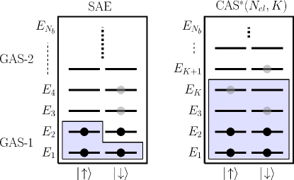
Figure 2: (color online). Generalized active spaces used in this work. The energies of the single-particle levels (up to $N_{b}$ spatial orbitals) are denoted by $E_{i}$. The two spin configurations, $|\uparrow\rangle$ and $|\downarrow\rangle$, are degenerate in the spin restricted HF ansatz. The left panel shows the SAE approximation, where only one electron ($\downarrow$ in level $E_{2}$ in this case) is allowed to be excited. The right panel shows the complete-active space (CAS^∗) situation, where correlation can be systematically built in with the incorporation of more and more active orbitals. $N_{el}$-electrons are allowed to occupy $K$ spatial orbitals and one electron excitations for any spin configuration are allowed above level $E_{K}$.

The relevant GAS partitions for this work are summarized in Fig. 2. The simplest approximation is the SAE approximation, in which only one selected electron may occupy excited Slater determinants, likewise the CIS approximation can be obtained from the GAS. By construction, no additional potentials are needed to be evaluated to obtain this widely used truncation. The other partition refers to the complete-active-space (CAS) concept Olsen et al. (1988); Helgaker et al. (2014), which corresponds to a FCI description (with possibly a frozen core) up to a spatial orbital index $K$. In the present TD-GASCI approach, the CAS is accompanied by additional single excitations out of the CAS, indicated in our notation by CAS${}^{*}(N_{el},K)$, where $N_{el}$ denotes the active electrons and $K$ the number of spatial orbitals within the CAS. In this context we wish to emphasize that we consider only one electron in the continuum throughout and double ionization is neglected, per construction of the GAS Bauch et al. (2014).

III Correlation effects in enhanced ionization

To study EI in molecules, we consider colinear models of $\mathrm{H}_{2}$ and $\mathrm{LiH}$. We use the regularized Coulomb potential between the electrons and the nuclei,

$$v(x,R)=-\frac{Z_{1}}{\sqrt{(x-\frac{R}{2})^{2}+s^{2}}}-\frac{Z_{2}}{\sqrt{(x+\frac{R}{2})^{2}+s^{2}}}\;.$$ (7)

Here $x$ is the electron coordinate, $R$ is the inter-nuclear distance, and $Z_{i}$ $(i=1,2)$ the nuclear charges. For all calculations we use the softening parameter, $s=1$. A two-electron model of $\mathrm{H}_{2}$ is defined by $Z_{1}=Z_{2}=1$ and a four electron model of $\mathrm{LiH}$ by $Z_{1}=1$, and $Z_{2}=3$. The electron-electron interaction in this model reads

$$w(x_{i},x_{j})=\frac{1}{\sqrt{(x_{i}-x_{j})^{2}+s^{2}}}\;.$$ (8)

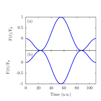
Figure 3: (color online). Normalized electric field with (a) $\varphi_{\textup{CEP}}=0$ and (b) $\varphi_{\textup{CEP}}=\pi$.

Such kind of models for diatomic molecules are well established in strong-field physics involving near-infrared fields Kulander et al. (1996). In the calculations we use the length gauge to describe the interaction with the laser field. We use the vector potential with a sine-square envelope Han and Madsen (2010),

$$A(t)=\frac{F_{0}}{\omega}\sin^{2}\Big{(}\frac{\pi t}{T}\Big{)}\sin{(\omega t+\varphi_{\textup{CEP}})}\qquad(0\leq t\leq T)\;,$$ (9)

where $T=n\frac{2\pi}{\omega}$ is the pulse duration with $n=1$, the number of cycles. The corresponding electric field is $F(t)=-\frac{\partial A(t)}{\partial t}$. $F_{0}$ is the maximum amplitude of the laser field to be specified below in the calculations, $\omega$ is the angular frequency and $\varphi_{\textup{CEP}}$ is the carrier-envelope-phase (CEP). The form of the laser pulse is shown in Fig. 3. For the present work we use 800 nm ($\omega=0.057$) and single-cycle pulses of duration $2.65$ fs ($110$ a.u.). The vector potential in Eq. (9) ensures that the time-integral over the electric field is vanishing, as it should be Madsen (2002). We note that the pulse duration considered here is so short that a molecule will not have time to dissociate to the range of critical inter-nuclear distances for EI during the presence of the pulse. Experimentally a pump-probe scheme is therefore required to investigate the EI phenomena for such short pulses.

To extract the total ionization probability, we add a complex absorbing potential (CAP) to the Hamiltonian,

$$H^{\textup{CAP}}(t)=H(t)-iV_{\textup{CAP}}\;,$$ (10)

where the CAP has the form Zanghellini et al. (2006)

$$V_{\textup{CAP}}(x)=1-\cos\left(\frac{\pi(|x|-x_{\textup{CAP}})}{2(x_{s}-x_{\textup{CAP}})}\right)\;,$$ (11)

for $|x|>x_{\textup{CAP}}$ and zero otherwise. For sufficiently long propagation time, $t_{f}$, after the end of pulse, the continuum part of the wave function has passed into the region of space beyond $x_{\textup{CAP}}$ and has been absorbed. The total ionization yield is then given by

$$\mathcal{P}(t_{f})=1-\mathcal{N}(t_{f})\;,$$ (12)

with $\mathcal{N}(t_{f})=\langle\Psi(t_{f})|\Psi(t_{f})\rangle$ Kulander (1987). To extract the ionization yield after the end of the pulse, we propagate the equations of motion to a final time, $t_{f}$ = 241 fs. We found that this time is sufficient to obtain converged results, also for correlated situations.

We partition the full simulation box into an inner (central) and an outer region. In the present simulation the main focus is on a wide range of inter-nuclear separations. Therefore, we need a relatively large box for the central region, $|x|<x_{c}$, as the correlated bound part of the wave function is described by localized HF and pseudo-orbitals. We use $x_{c}=16$ in the present calculation, cf. Fig. 1, and checked carefully for convergence of our results. We use 16 elements which have 8 DVR functions each for the central region which results in total 111 FE-DVR functions in the central region for all calculations. Further increasing the number of DVR functions leads to almost no change in the HF energy. The TD-GASCI calculation is done on the full simulation box to take into account the continuum. In the present calculation we set the box size to $x_{e}=200$, and the outer region is described by the FE-DVR functions. By using the same FE-DVR parameters as for the inner region, we therefore include 699 FE-DVR functions for the whole simulation box. We checked the convergence with respect to different box parameters and the above parameters gave converged results.

III.1 Two-electron $\mathrm{H}_{2}$-like molecule

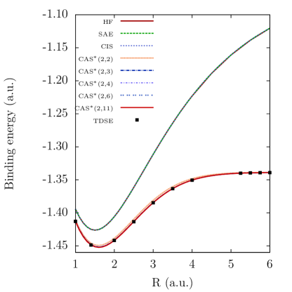
Figure 4: (color online). Total ground-state energy of the 2-electron $\mathrm{H}_{2}$-like molecule. In the upper curve the SAE and the CIS approximation overlap with the HF result. CAS${}^{*}(2,2)$ represents the TD-GASCI calculation with two active orbitals in the GAS. Similarly CAS${}^{*}(2,11)$ represents the TD-GASCI calculation with eleven active orbitals in the GAS.

The two electron system is the preferred choice of system to use to validate the approach because we can directly compare the results of the TD-GASCI simulations with TDSE simulations, which are performed in the same FE-DVR basis set. We begin with the ground state energy calculation with imaginary time propagation to demonstrate the features of the TD-GASCI method. In Fig. 4 we show the total ground state energy of 1D $\mathrm{H}_{2}$ with HF, SAE, CIS approximations and different GAS methods along with the TDSE calculations. Let us first discuss the approximations including singly excited determinants only. In the SAE approximation, the wave function reads

$$|\Psi_{\rm SAE}(t)\rangle=C_{0}(t)|\Phi_{0}\rangle+\sum_{a}C_{i}^{a}(t)|\Phi_{i}^{a}\rangle\;.$$ (13)

Here, $|\Phi_{0}\rangle$ is the HF reference determinant, and $|\Phi_{i}^{a}\rangle$ is a singly-excited determinant with the time-dependent CI-coefficients. In this approximation the sum runs over all virtual orbitals, $a$, with a fixed core orbital, $i$. Therefore, it represents the effective interaction felt by the electrons from the ionic core. In the CIS approximation the wave function reads

$$|\Psi_{\rm CIS}(t)\rangle=C_{0}(t)|\Phi_{0}\rangle+\sum_{i,a}C_{i}^{a}(t)|\Phi_{i}^{a}\rangle\;.$$ (14)

This approximation incorporates all possible single excitations from the core orbitals to the virtual orbitals. The time-dependent CIS approximation has been widely used for understanding the processes involving strong-field ionization Rohringer et al. (2006); Greenman et al. (2010); Karamatskou et al. (2014). Although these two approximations take into account a certain contribution to the correlation by accounting for the singly-excited determinants, the SAE and CIS approximations do not improve the ground state energy. This is according to Brillouin’s theorem Szabo and Ostlund (1996), which states that the matrix elements of the Hamiltonian between the reference state and singly-excited states vanish within a HF basis. From Fig. 4 we can see that the ground state energy curve obtained from the SAE and CIS approximations overlap with the HF ground state. Further, these approximations are unable to reproduce the correct dissociation limit due to the restricted HF ansatz used in this work, which prohibits dissociation into two open shell systems. For the GAS methods, the wave function is written as

$$|\Psi_{\rm GAS}(t)\rangle = C_{0}(t)|\Phi_{0}\rangle+\sum_{ia}C_{i}^{a}(t)|\Phi_{i}^{a}\rangle$$ (15)

$$+\frac{1}{4}\sum_{ijab}C_{ij}^{ab}(t)|\Phi_{ij}^{ab}\rangle+\cdots\;.$$

Let us consider the CAS${}^{*}(2,2)$ model with two active orbitals in the lowest GAS partition. It means, the summation over the core orbitals in Eq. (15) runs from one to two. Similarly, in the CAS${}^{*}(2,3)$ model we have three active orbitals and so on. With the CAS${}^{*}(2,2)$ model Fig. 4 shows that the ground state energy curve improves significantly over the SAE and CIS approximations and it tends to converge towards the exact TDSE ground state. We observe that the CAS${}^{*}(2,4)$ model with four active orbitals in the lowest GAS partition produces a converged result. In order to check the convergence, we further increased the number of active orbitals to six and then to eleven and found that the CAS${}^{*}(2,4)$ model is already converged. This is due to the multi-reference character of the CAS wave functions, which allows for the break up into two H atoms with singly-occupied orbitals. This is in contrast to the underlying restricted HF method, where orbitals are always doubly occupied.

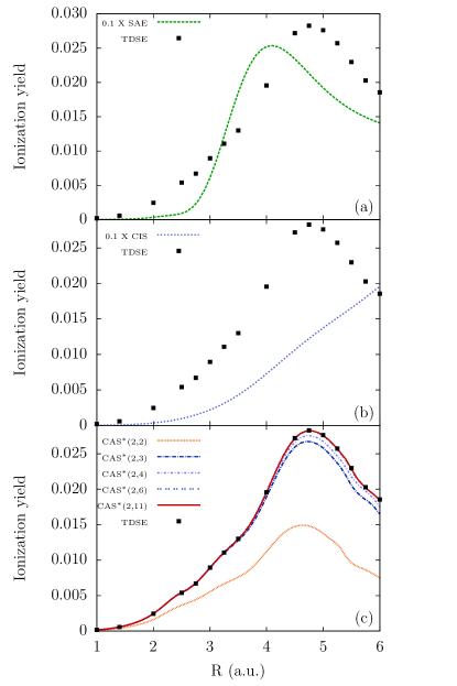
Figure 5: Ionization yield vs inter-nuclear distance $R$ for our model $\mathrm{H}_{2}$ with ${F}_{0}=0.05$ for (a) SAE approximation, (b) CIS approximation, and (c) GAS approximations. The CAS${}^{*}(2,2)$ model represents two active orbitals in the lowest GAS partition and similarly, e.g, the CAS${}^{*}(2,11)$ model incorporates eleven active orbitals in the lowest GAS partition. The squares are fully correlated TDSE reference data.

After the preparation of the $\mathrm{H}_{2}$-like molecule in its ground state by imaginary time propagation, we use the 800 nm laser pulse of Fig. 3 with $\varphi_{\textup{CEP}}=0$ and two different field strengths, (i) ${F}_{0}$ = 0.05 (8.75$\times 10^{14}$ W/cm²) and (ii) ${F}_{0}$ = 0.15 (7.87$\times 10^{15}$ W/cm²), to ionize the molecule. Since the $\mathrm{H}_{2}$ model is homonuclear, the $\varphi_{\textup{CEP}}=\pi$ field of Fig. 3(b) gives the same results for the ionization yield as $\varphi_{\textup{CEP}}=0$. In Fig. 5 we show the ionization yield as a function of the inter-nuclear separation. In Fig. 5(a) we compare the results between the SAE approximation and TDSE calculations. We have scaled down the SAE results by an order of magnitude. With the increase of the inter-nuclear distance, the ionization yield enhances in both models and then it gradually decreases. In the SAE approximation the EI peak is at $R=4.1$ which is well below the exact TDSE result of $R=4.7$. An earlier calculation on a similar 1D model observed the EI peak around the same inter-nuclear distance  Yu et al. (1996). The SAE approximation captures the overall behavior of EI but it overestimates largely the magnitude and peaks at the wrong position and, therefore, demonstrates the failure of the model to describe the EI phenomena quantitatively. The comparison between the CIS approximation and the TDSE calculation is shown Fig. 5(b). Similarly to SAE, the CIS yield is multiplied by $0.1$. The CIS approximation is unable to capture the feature of EI with the laser parameters used in the present calculation. It can describe the features qualitatively at the equilibrium separation, but the EI phenomena which occurs at large inter-nuclear separation can not be described.

In order to understand the electron correlation effects we turn to the discussion of Fig. 5(c). The lower curve corresponds to the CAS${}^{*}(2,2)$ model, i.e., two active orbitals in the lowest GAS partition, and one can see that this model predicts the correct EI behavior but the magnitude is much less than the corresponding TDSE value. Unlike the SAE and CIS approximations, the CAS${}^{*}(2,2)$ model nevertheless captures the correct position of the EI peak. By successively increasing the number of orbitals [CAS${}^{*}(2,3)$ to CAS${}^{*}(2,11)$ in Fig. 5], we achieve convergence of the ionization yield and observe perfect agreement with the TDSE calculations (squares). We find that at least six active orbitals in the GAS partition are needed to describe the EI phenomena quantitatively.

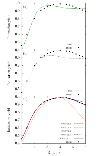
Figure 6: The same as Fig. 5, but for ${F}_{0}=0.15$.

In the next step, we increase the laser intensity to ${F}_{0}$ = 0.15 and observe that the CAS${}^{*}(2,6)$ model with six active orbitals is again the smallest GAS partition where the results converge to the TDSE results, see Fig. 6. The idea of introducing the GAS concept is to mitigate the computational constraint arising due to exponential scaling. By comparing with the exact TDSE results, we found, as expected, an enormous gain in terms of computational costs. To give an example, the converged CAS${}^{*}(2,6)$ calculations took 35 CPU hours on a 2.8 GHz Intel Ivy bridge CPU while the TDSE needed about 1400 CPU hours on an AMD Opteron CPU. Albeit the drastic reduction in CPU time, the TD-GASCI method with a limited number of active orbitals is still able to describe quantitatively the EI phenomena, including correlation.

III.2 Four-electron $\mathrm{LiH}$-like molecule

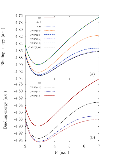
Figure 7: (color online). Binding energy of the $\mathrm{LiH}$ model. (a): HF, SAE and CIS approximations together with GAS calculations [CAS${}^{*}(2,\bullet)$] with two active electrons, (b): the same but with four active electrons in the CAS [CAS${}^{*}(4,\bullet)$].

We now turn our attention to the four-electron heteronuclear $\mathrm{LiH}$ molecule for which TDSE simulations of EI are infeasible. $\mathrm{LiH}$ lacks the reflection symmetry of $\mathrm{H}_{2}$ at the origin and thus strong CEP for few-cycle pulses can be expected.

We choose the geometric center as the origin of the coordinate system and choose $Z_{1}=1$ and $Z_{2}=3$ in Eq. (3), i.e., the $\mathrm{Li}$ atom is at $-R/2$ and the $\mathrm{H}$ atom is placed at $+R/2$. We prepare the $\mathrm{LiH}$-like molecule in its ground state by imaginary time propagation. All numerical parameters are the same as for $\mathrm{H}_{2}$, see Sec. III.1.

III.2.1 Ground-state energies

The ground state energy curve for $\mathrm{LiH}$ is shown in Fig. 7. In Panel (a) the HF, SAE and CIS approximations with CAS${}^{*}(2,\bullet)$ approximations involving two active electrons are shown. Similar to $\mathrm{H}_{2}$, the multi-reference description is essential and SAE and CIS fail to reproduce the correct dissociation limit. We find that a CAS${}^{*}(2,5)$ is sufficient for two active electrons, as seen by comparison with the CAS${}^{*}(2,10)$ calculation. To test the frozen-core approximation, we use four active electrons and obtain the converged result for the ground state energy, as shown in panel (b). As expected, the energy is lowered but the equilibrium distance is around the same internuclear distance. Similar to Ref. Bauch et al. (2014), the CAS${}^{*}(4,5)$ with five active orbitals produces the converged ground state energy curve.

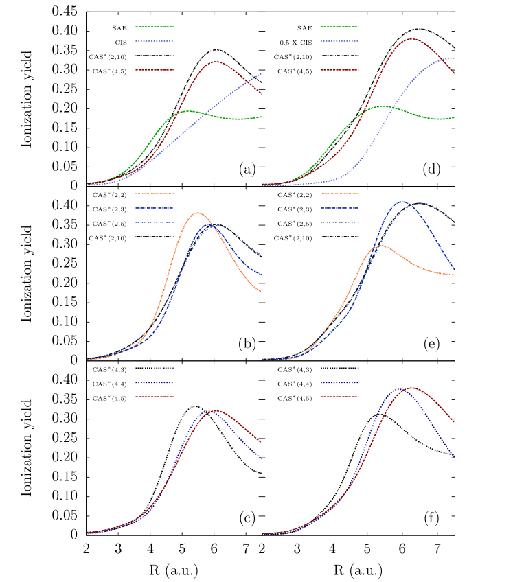
Figure 8: Ionization yield vs inter-nuclear distance $R$ for $\mathrm{LiH}$ with ${F}_{0}=0.025$. In panels (a-c), $\varphi_{\textup{CEP}}=0$, for (d-f) $\varphi_{\textup{CEP}}=\pi$ (see Fig. 3). (a) and (d) Comparison between SAE, CIS approximations and fully converged GAS methods with two and four active electrons. (b) and (e) Comparison between different GAS methods with two active electrons. (c) and (f) Comparison between different GAS methods with four active electrons.

III.2.2 Enhanced ionization

In order to understand the correlation effects in EI phenomena, we expose the $\mathrm{LiH}$ molecule to a laser pulse with field strength ${F}_{0}=0.025$ (2.18$\times 10^{13}$ W/cm²) for $\varphi_{\textup{CEP}}=0$ and $\varphi_{\textup{CEP}}=\pi$ [Fig. 3]. This choice is equivalent to the two possible orientations in 1D of the molecule w.r.t. the dominant half-cycle. In Figs. 8(a-c), we show the EI calculation with $\varphi_{\textup{CEP}}=0$. We compare the results of the SAE, CIS approximations and two GAS methods with two and four active electrons in Fig. 8(a). The SAE approximation shows the EI peak at $R=5.2$. Like in the case of $\mathrm{H_{2}}$, the SAE approximation predicts the EI phenomena for $\mathrm{LiH}$, but again the CIS approximation fails to describe the EI phenomena. In Fig. 8(b), we show different GAS calculations with two active outer electrons. The CAS${}^{*}(2,2)$ model does not predict the correct EI peak position and it overestimates the magnitude of the ionization yield. Further increasing the number of active orbitals to three we found that the EI peak is shifted towards larger inter-nuclear separation. We systematically increased the number of active orbitals and found that we need at least five active orbitals to obtain converged results for EI. The converged EI peak is at $R=6.1$ with the CAS${}^{*}(2,5)$ model. To check this convergence we increase the number of active orbitals to ten and the observed yield shows a trend of convergence. In Fig. 8(c) we show the results with four active electrons in the GAS partition and the CAS${}^{*}(4,5)$ model with five active orbitals in the GAS partition leads to a converged result. The CAS${}^{*}(4,5)$ model predicts the same qualitative behavior like the CAS${}^{*}(2,5)$ model. The EI peak in the CAS${}^{*}(2,5)$ and the CAS${}^{*}(4,5)$ models have the same position but the magnitude is different. In terms of computational cost the CAS${}^{*}(4,5)$ model is much more expensive than CAS${}^{*}(2,5)$. To give an example the CAS${}^{*}(4,5)$ model took 530 CPU hours compared to 24 hours of the CAS${}^{*}(2,5)$ model on a 2.8 GHz Intel Ivy bridge CPU. Thus using only two active electrons in the GAS partition gives us more than a 20 times reduction in the computational cost, a tremendous gain.

In Figs. 8(d-f), we show the EI calculation with $\varphi_{\textup{CEP}}=\pi$, and the conclusions w.r.t. convergence are the same as for Figs. 8 (a-c). As we incorporate more correlation the yield is converged with five active orbitals. In Ref. Bauch et al. (2014) it was shown that the ionization yield at equilibrium is larger for $\varphi_{\textup{CEP}}=0$ compared to $\varphi_{\textup{CEP}}=\pi$ . We observe that the ionization yield with $\varphi_{\textup{CEP}}=\pi$ is consistently greater than with $\varphi_{\textup{CEP}}=0$ at the critical inter-nuclear separation in the different GAS calculations. It certainly illustrates the importance of correlation contributions in the direction of electron emission from a polar molecule like $\mathrm{LiH}$.

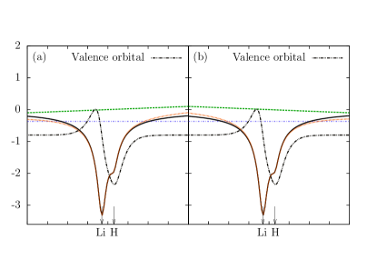
Figure 9: (color online). Sketch of the strong-field ionization scenarios of the $\mathrm{LiH}$ model. Shown are the binding potential (black solid lines) and the modified potential (red dotted lines) by the electrical field (green dashed lines) at the peak of the single-cycle pusle F(t) along with the valence orbital (black dashed dotted). The orbital energy is indicated by the blue horizontal line. Panel (a) is for $\varphi_{\textup{CEP}}$ = 0, (b) for $\varphi_{\textup{CEP}}=\pi$ (see Fig. 3).

III.3 CEP effects in EI of $\mathrm{LiH}$

In this section, we discuss the CEP effects in EI. The importance of the CEP of the few-cycle pulse in EI of polar molecules was demonstrated on a one-electron system, $\mathrm{HeH}{}^{2+}$ in Ref. Kamta and Bandrauk (2005, 2007) and on a two-electron system, $\mathrm{HeH}{}^{+}$ in Ref. Dehghanian et al. (2013). In this work we illustrate the importance of CEP effects in EI in the four-electron $\mathrm{LiH}$ model. As alluded in the beginning of Sec. III, to observe such CEP effects experimentally would require a pump-probe scheme. The $\mathrm{LiH}$-like molecule can have two orientations w.r.t the linearly polarized laser field.

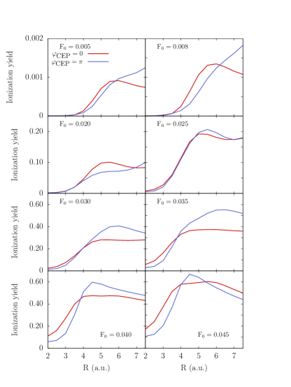
Figure 10: (color online). Ionization yield vs inter-nuclear distance $R$ for the $\mathrm{LiH}$ model in the SAE approximation. See Fig. 3. for the definition of $\varphi_{\textup{CEP}}$. The panel with ${F}_{0}=0.005$ is multiplied by a factor of ten to scale.

Figure 11: (color online). Ionization yield vs inter-nuclear distance $R$ for the $\mathrm{LiH}$ model in the CAS${}^{*}(2,5)$ model. See Fig. 3. for the definition of $\varphi_{\textup{CEP}}$. The panel with ${F}_{0}=0.005$ is multiplied by a factor of ten to scale.

In Fig. 9, we show a schematic diagram of $\mathrm{LiH}$ interacting with a laser field. The interaction with ${F(t)}$ at the peak of the pulse with $\varphi_{\textup{CEP}}=0$ [Fig. 3(a)] is illustrated in Fig. 9(a) and with $\varphi_{\textup{CEP}}=\pi$ [Fig. 3(b)] in Fig. 9(b), together with the field-free valence HF orbital. To study the CEP effects, the intensities are chosen to illustrate the correlation effects in the EI phenomena in the tunneling as well as in the over-barrier-ionization regime. First we use ${F}_{0}=0.005$, $0.008$ which are below the over-barrier-field strength and represents the tunneling regime and the others with ${F}_{0}=0.020$, up to $0.045$, which are above the over-barrier-field strengths.

The CEP effects in the EI are shown in Figs. 10 (SAE) and 11 [correlated CAS${}^{*}(2,5)$]. In the tunneling regime, the EI with $\varphi_{\textup{CEP}}=0$ shows a completely different trend than with the $\varphi_{\textup{CEP}}=\pi$. The EI peak is well captured with $\varphi_{\textup{CEP}}=0$, but with $\varphi_{\textup{CEP}}=\pi$ it is absent at the expected inter-nuclear separation. The same feature is observed with the CAS${}^{*}(2,5)$ model in Fig. 11. The correlated model predicts a larger ionization yield at the critical inter-nuclear separation than the SAE approximation. It is important to emphasize that the EI peak is shifted towards larger inter-nuclear separation with $\varphi_{\textup{CEP}}=\pi$. This is a CEP effect because both, the SAE and the CAS${}^{*}(2,5)$ approximations, predicts the same trend. As we increase the field strength to $F_{0}=0.025$, the SAE approximation predicts the EI peak for both $\varphi_{\textup{CEP}}$ at similar inter-nuclear separation. However, in the SAE approximation there is a cross-over between the EI peak with two different $\varphi_{\textup{CEP}}$. As we increase the intensity, the SAE approximation predicts more ionization yield with $\varphi_{\textup{CEP}}=\pi$ than with $\varphi_{\textup{CEP}}=0$ at the critical inter-nuclear separation. The correlated model gives a completely different picture. In this model, the ionization yield is larger for $\varphi_{\textup{CEP}}=0$ than for $\varphi_{\textup{CEP}}=\pi$ for $F_{0}>0.035$, which is certainly due to correlation effects. The previous calculations with one- and two-electron molecules predict larger ionization yield with the $\varphi_{\textup{CEP}}=0$ than with $\varphi_{\textup{CEP}}=\pi$ at the critical inter-nuclear separation Kamta and Bandrauk (2005, 2007); Dehghanian et al. (2013). However, our studies show that there exists a cross-over between the $\varphi_{\textup{CEP}}=0$ and $\varphi_{\textup{CEP}}=\pi$ cases in the over-barrier regime as well as the $\varphi_{\textup{CEP}}=\pi$ predicts more ionization yield than with $\varphi_{\textup{CEP}}=0$ in the tunneling regime. Therefore the CEP of a few-cycle pulse plays an important role in describing the direction of electron ejection in both tunneling and over-barrier-ionization, and most importantly the electron correlation can completely reverse the trend of the SAE approximation as seen from, e.g, the $F_{0}=0.035$ case.

IV Summary and Conclusion

In this work, we investigated the importance of electron correlation effects in enhanced ionization of model diatomic molecules by using the TD-GASCI method. The strength of the TD-GASCI method is to incorporate the electron correlation systematically. We used 1D models of $\mathrm{H}_{2}$ and $\mathrm{LiH}$ to study the electron correlation effects. We used the imaginary time propagation to calculate the ground state of the molecules. We then gave a detailed analysis of EI with different laser intensities and illustrated the features that arise because of electron correlation by using the TD-GASCI method. We found that correlation is very important to describe the EI behavior in the $\mathrm{H}_{2}$ model. The SAE approximation failed to describe EI in $\mathrm{H}_{2}$ model and we would expect the same trends in real 3D systems. Another important conclusion from our study is the failure of the CIS approximation to correctly describe the EI phenomena. On the other hand the different GAS approximations predicted the correct behavior of EI and as we incorporated more and more correlation in the H₂ model the result converged towards the TDSE calculations. For the LiH model we found that EI persists and that the correlation shifts the peak of the EI towards larger inter-nuclear separation. We also estimated the computational cost to solve the TD-GASCI equations with different GAS partitioning and found that it is computationally feasible and inexpensive compared to TDSE calculations. We emphasized the advantage of two active electrons over four active electrons in the GAS partition for the particular problem of strong-field ionization where the valence electrons play a dominant role. Compared to the exact four electrons in the GAS partition, the two active electron model predicts the yield correctly and with much less computational cost. The CEP of a few-cycle pulse plays an important role in describing the EI in the asymmetric $\mathrm{LiH}$ model. The intriguing feature is the cross-over between the $\varphi_{\textup{CEP}}=0$ and $\varphi_{\textup{CEP}}=\pi$ in the tunneling as well as in over-barrier-ionization regime. In conclusion the electron correlation plays a crucial role in the EI phenomena.