\authorinfo

Further author information: E-mail: kkatop@lab.tamagawa.ac.jp

Quasi-Bell entangled coherent states and its quantum discrimination problem in the presence of thermal noise

Kentaro Kato \skiplinehalfQuantum Communication Research Center   
Quantum ICT Research Institute
   Tamagawa University   
Tamagawa-gakuen 6-1-1
   Machida    Tokyo 194-8610 JAPAN
Abstract

The so-called quasi-Bell entangled coherent states in a thermal environment are studied. In the analysis, we assume thermal noise affects only one of the two modes of each state. First the matrix representation of the density operators of the quasi-Bell entangled coherent states in a thermal environment is derived. Secondly we investigate the entanglement property of one of the quasi-Bell entangled coherent states with thermal noise. At that time a lower bound of the entanglement of formation for the state is computed. Thirdly the minimax discrimination problem for two cases of the binary set of the quasi-Bell entangled coherent states with thermal noise is considered, and the error probabilities of the minimax discrimination for the two cases are computed with the help of Helstrom’s algorithm for finding the Bayes optimal error probability of binary states.

keywords:
Entangled Coherent State, Decoherence, Thermal Noise, Quantum Detection Theory

1 Introduction

The choice or design of quantum states for information-processing resource is one of important issues to build a useful quantum information system that breaks the performance limit of classical schemes in information-communication technologies or that possesses quite new functions. Entanglement may be one of potential phenomena and indeed various types of entangled states have been widely discussed from the point of view of both theory and experiment and from fundamental properties to its applications. Toward developing macroscopic quantum information-communication technologies, we are interested in entangled coherent states [1, 2]. Above all, our interest is focused on the so-called quasi-Bell entangled coherent states in this paper. The quasi-Bell entangled coherent states are defined as a set of the following four superpositions of two-mode coherent states: |α,±α12+|α,α12subscriptket𝛼plus-or-minus𝛼12subscriptket𝛼minus-or-plus𝛼12|{\alpha,\pm\alpha}\rangle_{12}+|{-\alpha,\mp\alpha}\rangle_{12} and |α,±α12|α,α12subscriptket𝛼plus-or-minus𝛼12subscriptket𝛼minus-or-plus𝛼12|{\alpha,\pm\alpha}\rangle_{12}-|{-\alpha,\mp\alpha}\rangle_{12} [3].

In an ideal situation, it has been clarified that the quasi-Bell entangled coherent states are applicable to several applications. For example, teleportation and computation by the quasi-Bell entangled coherent states were already proposed [4, 5, 6, 7]. The error-free quantum reading scheme was proposed by Hirota [8], where phase-shift keying (PSK) format was used for its signal modulation. In order to realise such information-communication systems, more precise analysis of the states in various realistic situations is needed. In other words, our central concern is whether or not the quasi-Bell entangled coherent states are still applicable to information-communication technologies even in practical situations. For this question, the effect of channel loss to the quasi-Bell entangled coherent states was reported by present author in the context of the quantum reading in SPIE Optics+Photonics 2013 [9]. In line with this thought, we aim to clarify the effect of thermal noise for the quasi-Bell entangled coherent states.

This paper is organized as follows. Section 2 reviews the basics of the quasi-Bell entangled coherent states when there is no noise. In Section 3, we derive the matrix representation of the density operators of the quasi-Bell entangled coherent states in a thermal environment by using the thermalizing operator. The degree of entanglement of one of the quasi-Bell entangled coherent states with thermal noise is discussed in Section 4, and an optimal quantum discrimination problem for two cases of the binary set of the quasi-Bell entangled coherent states with thermal noise is considered in Section 5. In these sections, we execute computer simulations by using the matrix representation mentioned in Section 3. Section 6 summarizes our results obtained in this paper.

2 Quasi-Bell Entangled Coherent States without thermal noise

Consider two modes of electromagnetic field with corresponding annihilation operators a^1subscript^𝑎1\hat{a}_{1} and a^2subscript^𝑎2\hat{a}_{2}. Two-mode coherent states are defined by |α1,α212=D^1(α1)D^2(α2)|0,012,subscriptketsubscript𝛼1subscript𝛼212subscript^𝐷1subscript𝛼1subscript^𝐷2subscript𝛼2subscriptket0012|{\alpha_{1},\alpha_{2}}\rangle_{12}=\hat{D}_{1}(\alpha_{1})\hat{D}_{2}(\alpha_{2})|{0,0}\rangle_{12}, where |0,012subscriptket0012|{0,0}\rangle_{12} is the two-mode vacuum state and D^i(αi)=exp[αia^iαa^i]subscript^𝐷𝑖subscript𝛼𝑖subscript𝛼𝑖superscriptsubscript^𝑎𝑖superscript𝛼subscript^𝑎𝑖\hat{D}_{i}(\alpha_{i})=\exp[\alpha_{i}\hat{a}_{i}^{\dagger}-\alpha^{\ast}\hat{a}_{i}] is the displacement operator of the mode i𝑖i (i=1,2𝑖12i=1,2). The state |α1,α212subscriptketsubscript𝛼1subscript𝛼212|{\alpha_{1},\alpha_{2}}\rangle_{12} can be expressed into the form

|α1,α212=exp[|α1|22|α2|22]n1=0n2=0α1n1α2n2n1!n2!|n1,n212,subscriptketsubscript𝛼1subscript𝛼212superscriptsubscript𝛼122superscriptsubscript𝛼222superscriptsubscriptsubscript𝑛10superscriptsubscriptsubscript𝑛20superscriptsubscript𝛼1subscript𝑛1superscriptsubscript𝛼2subscript𝑛2subscript𝑛1subscript𝑛2subscriptketsubscript𝑛1subscript𝑛212|{\alpha_{1},\alpha_{2}}\rangle_{12}=\exp[-\frac{|\alpha_{1}|^{2}}{2}-\frac{|\alpha_{2}|^{2}}{2}]\sum_{n_{1}=0}^{\infty}\sum_{n_{2}=0}^{\infty}\frac{\alpha_{1}^{n_{1}}\alpha_{2}^{n_{2}}}{\sqrt{n_{1}!n_{2}!}}|{n_{1},n_{2}}\rangle_{12}, (1)

where |n1,n212subscriptketsubscript𝑛1subscript𝑛212|{n_{1},n_{2}}\rangle_{12} are two-mode Fock states. The quasi-Bell entangled coherent states are defined by the following superpositions of two-mode coherent states [3].

|𝚽112subscriptketsubscript𝚽112\displaystyle|{\boldsymbol{\Phi}_{1}}\rangle_{\rm 12} =\displaystyle= 𝒩+(|β,β12+|β,β12),subscript𝒩subscriptket𝛽𝛽12subscriptket𝛽𝛽12\displaystyle\mathcal{N}_{+}\left(|{\beta,\beta}\rangle_{\rm 12}+|{-\beta,-\beta}\rangle_{\rm 12}\right), (2)
|𝚽212subscriptketsubscript𝚽212\displaystyle|{\boldsymbol{\Phi}_{2}}\rangle_{\rm 12} =\displaystyle= 𝒩(|β,β12|β,β12),subscript𝒩subscriptket𝛽𝛽12subscriptket𝛽𝛽12\displaystyle\mathcal{N}_{-}\left(|{\beta,\beta}\rangle_{\rm 12}-|{-\beta,-\beta}\rangle_{\rm 12}\right), (3)
|𝚽312subscriptketsubscript𝚽312\displaystyle|{\boldsymbol{\Phi}_{3}}\rangle_{\rm 12} =\displaystyle= 𝒩+(|β,β12+|β,β12),subscript𝒩subscriptket𝛽𝛽12subscriptket𝛽𝛽12\displaystyle\mathcal{N}_{+}\left(|{\beta,-\beta}\rangle_{\rm 12}+|{-\beta,\beta}\rangle_{\rm 12}\right), (4)
|𝚽412subscriptketsubscript𝚽412\displaystyle|{\boldsymbol{\Phi}_{4}}\rangle_{\rm 12} =\displaystyle= 𝒩(|β,β12|β,β12),subscript𝒩subscriptket𝛽𝛽12subscriptket𝛽𝛽12\displaystyle\mathcal{N}_{-}\left(|{\beta,-\beta}\rangle_{\rm 12}-|{-\beta,\beta}\rangle_{\rm 12}\right), (5)

where 𝒩±=1/2(1±exp[4|β|2])subscript𝒩plus-or-minus12plus-or-minus14superscript𝛽2\mathcal{N}_{\pm}={1}/{\sqrt{2(1\pm\exp[-4|\beta|^{2}])}} is the normalizing factors. From these expressions of the states, one can find the relations

|𝚽312=(1^1R^2(π))|𝚽112,|𝚽412=(1^1R^2(π))|𝚽212,formulae-sequencesubscriptketsubscript𝚽312tensor-productsubscript^11subscript^𝑅2𝜋subscriptketsubscript𝚽112subscriptketsubscript𝚽412tensor-productsubscript^11subscript^𝑅2𝜋subscriptketsubscript𝚽212|{\boldsymbol{\Phi}_{3}}\rangle_{\rm 12}=(\hat{1}_{1}\otimes\hat{R}_{2}(\pi))|{\boldsymbol{\Phi}_{1}}\rangle_{\rm 12},\qquad|{\boldsymbol{\Phi}_{4}}\rangle_{\rm 12}=(\hat{1}_{1}\otimes\hat{R}_{2}(\pi))|{\boldsymbol{\Phi}_{2}}\rangle_{\rm 12}, (6)

where R^2(π)=exp[iπa^2a^2]subscript^𝑅2𝜋i𝜋superscriptsubscript^𝑎2subscript^𝑎2\hat{R}_{2}(\pi)=\exp[-{\rm i}\pi\hat{a}_{2}^{\dagger}\hat{a}_{2}] is the π𝜋\pi-rotation operator. In the context of optical communications, this property is understood as the PSK format of laser light.

The average numbers of photons for the states 𝚽1subscript𝚽1\boldsymbol{\Phi}_{1} and 𝚽3subscript𝚽3\boldsymbol{\Phi}_{3} are given by

n(𝚽1)=n(𝚽3)delimited-⟨⟩𝑛subscript𝚽1delimited-⟨⟩𝑛subscript𝚽3\displaystyle\langle n(\boldsymbol{\Phi}_{1})\rangle=\langle n(\boldsymbol{\Phi}_{3})\rangle =\displaystyle= 2|β|2tanh[2|β|2].2superscript𝛽22superscript𝛽2\displaystyle 2|\beta|^{2}\tanh[2|\beta|^{2}]. (7)

It is easy to see that n(𝚽1)=n(𝚽3)0delimited-⟨⟩𝑛subscript𝚽1delimited-⟨⟩𝑛subscript𝚽30\langle n(\boldsymbol{\Phi}_{1})\rangle=\langle n(\boldsymbol{\Phi}_{3})\rangle\to 0 when β0𝛽0\beta\to 0. Similarly, the average numbers of photons for the states 𝚽2subscript𝚽2\boldsymbol{\Phi}_{2} and 𝚽4subscript𝚽4\boldsymbol{\Phi}_{4} are given by

n(𝚽2)=n(𝚽4)delimited-⟨⟩𝑛subscript𝚽2delimited-⟨⟩𝑛subscript𝚽4\displaystyle\langle n(\boldsymbol{\Phi}_{2})\rangle=\langle n(\boldsymbol{\Phi}_{4})\rangle =\displaystyle= 2|β|2coth[2|β|2],2superscript𝛽2hyperbolic-cotangent2superscript𝛽2\displaystyle 2|\beta|^{2}\coth[2|\beta|^{2}], (8)

and n(𝚽2)=n(𝚽4)1delimited-⟨⟩𝑛subscript𝚽2delimited-⟨⟩𝑛subscript𝚽41\langle n(\boldsymbol{\Phi}_{2})\rangle=\langle n(\boldsymbol{\Phi}_{4})\rangle\to 1 when β0𝛽0\beta\to 0. Symbol n(𝚽i)delimited-⟨⟩𝑛subscript𝚽𝑖\langle n(\boldsymbol{\Phi}_{i})\rangle is abbreviated to ndelimited-⟨⟩𝑛\langle n\rangle if it is clear from the context.

The set of the inner products of the quasi-Bell entangled coherent states forms the following Gram matrix.

𝖦=[𝚽1|𝚽11212𝚽1|𝚽21212𝚽1|𝚽31212𝚽1|𝚽41212𝚽2|𝚽11212𝚽2|𝚽21212𝚽2|𝚽31212𝚽2|𝚽41212𝚽3|𝚽11212𝚽3|𝚽21212𝚽3|𝚽31212𝚽3|𝚽41212𝚽4|𝚽11212𝚽4|𝚽21212𝚽4|𝚽31212𝚽4|𝚽41212]=[10K1300100K130100001],{\sf G}=\left[\begin{array}[]{cccc}{}_{\rm 12}\langle{\boldsymbol{\Phi}_{1}}|{\boldsymbol{\Phi}_{1}}\rangle_{\rm 12}&{}_{\rm 12}\langle{\boldsymbol{\Phi}_{1}}|{\boldsymbol{\Phi}_{2}}\rangle_{\rm 12}&{}_{\rm 12}\langle{\boldsymbol{\Phi}_{1}}|{\boldsymbol{\Phi}_{3}}\rangle_{\rm 12}&{}_{\rm 12}\langle{\boldsymbol{\Phi}_{1}}|{\boldsymbol{\Phi}_{4}}\rangle_{\rm 12}\\ {}_{\rm 12}\langle{\boldsymbol{\Phi}_{2}}|{\boldsymbol{\Phi}_{1}}\rangle_{\rm 12}&{}_{\rm 12}\langle{\boldsymbol{\Phi}_{2}}|{\boldsymbol{\Phi}_{2}}\rangle_{\rm 12}&{}_{\rm 12}\langle{\boldsymbol{\Phi}_{2}}|{\boldsymbol{\Phi}_{3}}\rangle_{\rm 12}&{}_{\rm 12}\langle{\boldsymbol{\Phi}_{2}}|{\boldsymbol{\Phi}_{4}}\rangle_{\rm 12}\\ {}_{\rm 12}\langle{\boldsymbol{\Phi}_{3}}|{\boldsymbol{\Phi}_{1}}\rangle_{\rm 12}&{}_{\rm 12}\langle{\boldsymbol{\Phi}_{3}}|{\boldsymbol{\Phi}_{2}}\rangle_{\rm 12}&{}_{\rm 12}\langle{\boldsymbol{\Phi}_{3}}|{\boldsymbol{\Phi}_{3}}\rangle_{\rm 12}&{}_{\rm 12}\langle{\boldsymbol{\Phi}_{3}}|{\boldsymbol{\Phi}_{4}}\rangle_{\rm 12}\\ {}_{\rm 12}\langle{\boldsymbol{\Phi}_{4}}|{\boldsymbol{\Phi}_{1}}\rangle_{\rm 12}&{}_{\rm 12}\langle{\boldsymbol{\Phi}_{4}}|{\boldsymbol{\Phi}_{2}}\rangle_{\rm 12}&{}_{\rm 12}\langle{\boldsymbol{\Phi}_{4}}|{\boldsymbol{\Phi}_{3}}\rangle_{\rm 12}&{}_{\rm 12}\langle{\boldsymbol{\Phi}_{4}}|{\boldsymbol{\Phi}_{4}}\rangle_{\rm 12}\end{array}\right]=\left[\begin{array}[]{cccc}1&0&K_{13}&0\\ 0&1&0&0\\ K_{13}&0&1&0\\ 0&0&0&1\end{array}\right], (9)

where the entry K13=sech[2|β|2]subscript𝐾13sechdelimited-[]2superscript𝛽2K_{13}={\rm sech}[2|\beta|^{2}]. From this matrix, it is noticed that the states 𝚽1subscript𝚽1\boldsymbol{\Phi}_{1} and 𝚽3subscript𝚽3\boldsymbol{\Phi}_{3} are non-orthogonal, while any other pair is orthogonal. The orthogonality of the states 𝚽2subscript𝚽2\boldsymbol{\Phi}_{2} and 𝚽4subscript𝚽4\boldsymbol{\Phi}_{4} is utilized to propose an error-free binary PSK quantum reading [8]. Indeed, the minimum probability of error (in terms of the minimax discrimination problem [10, 11, 12]) for the states 𝚽2subscript𝚽2\boldsymbol{\Phi}_{2} and 𝚽4subscript𝚽4\boldsymbol{\Phi}_{4} is

P¯e(𝚽2,𝚽4)superscriptsubscript¯𝑃esubscript𝚽2subscript𝚽4\displaystyle\bar{P}_{\rm e}^{\circ}(\boldsymbol{\Phi}_{2},\boldsymbol{\Phi}_{4}) =\displaystyle= max{p2+p4=1;p20;p40}[12(114p2p4|𝚽2|𝚽41212|2)]=0,\displaystyle\max_{\{p_{2}+p_{4}=1;p_{2}\geq 0;p_{4}\geq 0\}}\left[\frac{1}{2}\left(1-\sqrt{1-4p_{2}p_{4}\bigl{|}{}_{\rm 12}\langle{\boldsymbol{\Phi}_{2}}|{\boldsymbol{\Phi}_{4}}\rangle_{\rm 12}\bigr{|}^{2}}\right)\right]=0, (10)

while the minimum probability of error for the states 𝚽1subscript𝚽1\boldsymbol{\Phi}_{1} and 𝚽3subscript𝚽3\boldsymbol{\Phi}_{3} is

P¯e(𝚽1,𝚽3)superscriptsubscript¯𝑃esubscript𝚽1subscript𝚽3\displaystyle\bar{P}_{\rm e}^{\circ}(\boldsymbol{\Phi}_{1},\boldsymbol{\Phi}_{3}) =\displaystyle= max{p1+p3=1;p10;p30}[12(114p1p3|𝚽1|𝚽31212|2)]=exp[4|β|2]1+exp[4|β|2].\displaystyle\max_{\{p_{1}+p_{3}=1;p_{1}\geq 0;p_{3}\geq 0\}}\left[\frac{1}{2}\left(1-\sqrt{1-4p_{1}p_{3}\bigl{|}{}_{\rm 12}\langle{\boldsymbol{\Phi}_{1}}|{\boldsymbol{\Phi}_{3}}\rangle_{\rm 12}\bigr{|}^{2}}\right)\right]=\frac{\exp[-4|\beta|^{2}]}{1+\exp[-4|\beta|^{2}]}. (11)

It is well known that the states 𝚽2subscript𝚽2\boldsymbol{\Phi}_{2} and 𝚽4subscript𝚽4\boldsymbol{\Phi}_{4} are maximally entangled states [3]. The degrees of entanglement of the quasi-Bell entangled coherent states are given by

E(|𝚽112)=E(|𝚽312)𝐸subscriptketsubscript𝚽112𝐸subscriptketsubscript𝚽312\displaystyle{E}(|{\boldsymbol{\Phi}_{1}}\rangle_{\rm 12})={E}(|{\boldsymbol{\Phi}_{3}}\rangle_{\rm 12}) =\displaystyle= (1+K132)log2[1+K132](1K132)log2[1K132],1subscript𝐾132subscript21subscript𝐾1321subscript𝐾132subscript21subscript𝐾132\displaystyle-\left(\frac{1+K_{13}}{2}\right)\log_{2}\left[\frac{1+K_{13}}{2}\right]-\left(\frac{1-K_{13}}{2}\right)\log_{2}\left[\frac{1-K_{13}}{2}\right], (12)
E(|𝚽212)=E(|𝚽412)𝐸subscriptketsubscript𝚽212𝐸subscriptketsubscript𝚽412\displaystyle{E}(|{\boldsymbol{\Phi}_{2}}\rangle_{\rm 12})={E}(|{\boldsymbol{\Phi}_{4}}\rangle_{\rm 12}) =\displaystyle= 1,1\displaystyle 1, (13)

where we have used the entropy of entanglement [13, 14] defined by

E(|𝚽12)=Tr1(ρ^1log2ρ^1)=Tr2(ρ^2log2ρ^2)𝐸subscriptket𝚽12subscriptTr1subscript^𝜌1subscript2subscript^𝜌1subscriptTr2subscript^𝜌2subscript2subscript^𝜌2E(|{\boldsymbol{\Phi}}\rangle_{\rm 12})=-{\rm Tr}_{\rm 1}\left(\hat{{\rho}}_{\rm 1}\log_{2}\hat{{\rho}}_{\rm 1}\right)=-{\rm Tr}_{\rm 2}\left(\hat{{\rho}}_{\rm 2}\log_{2}\hat{{\rho}}_{\rm 2}\right) (14)

with the reduced density operators ρ^1=Tr2|𝚽12𝚽|subscript^𝜌1subscriptTr2subscriptket𝚽12bra𝚽\hat{{\rho}}_{\rm 1}={\rm Tr}_{\rm 2}|{\boldsymbol{\Phi}}\rangle_{\rm 12}\langle{\boldsymbol{\Phi}}| and ρ^2=Tr1|𝚽12𝚽|subscript^𝜌2subscriptTr1subscriptket𝚽12bra𝚽\hat{{\rho}}_{\rm 2}={\rm Tr}_{\rm 1}|{\boldsymbol{\Phi}}\rangle_{\rm 12}\langle{\boldsymbol{\Phi}}|. Eq.(13) shows that 𝚽2subscript𝚽2\boldsymbol{\Phi}_{2} and 𝚽4subscript𝚽4\boldsymbol{\Phi}_{4} are maximally entangled when there is no noise.

3 Quasi-Bell entangled coherent states in a thermal environment

In this section, we give the matrix representation of the density operators of the quasi-Bell entangled coherent states in a thermal environment. For this aim, we use the thermalizing operator [15, 16] 𝐓^(θ)^𝐓𝜃\hat{\bf T}(\theta) defined by

𝐓^(θ)=exp[θ(a^a~a^a~)].^𝐓𝜃𝜃^𝑎~𝑎superscript^𝑎superscript~𝑎\hat{\bf T}(\theta)=\exp[-\theta(\hat{a}\tilde{a}-\hat{a}^{\dagger}\tilde{a}^{\dagger})]. (15)

In this definition, a^^𝑎\hat{a} is the annihilation operator of the real mode to be primary investigated, and a~~𝑎\tilde{a} is the annihilation operator of the fictitious mode that satisfy [a^,a~]=0=[a^,a~]^𝑎~𝑎0^𝑎superscript~𝑎[\hat{a},\tilde{a}]=0=[\hat{a},\tilde{a}^{\dagger}] and [a~,a~]=1^~𝑎superscript~𝑎^1[\tilde{a},\tilde{a}^{\dagger}]=\hat{1}. Further, coshθ=1/1eω/kBT,𝜃11superscripte𝜔subscript𝑘B𝑇\cosh\theta={1}/{\sqrt{1-{\rm e}^{-\omega/k_{\rm B}T}}}, and sinhθ=1/eω/kBT1𝜃1superscripte𝜔subscript𝑘B𝑇1\sinh\theta={1}/{\sqrt{{\rm e}^{\omega/k_{\rm B}T}-1}} with frequency ω𝜔\omega, Boltzmann constant kBsubscript𝑘Bk_{\rm B}, and temperature T𝑇T. By using the thermalizing operator, various types of thermal states can be considered: (i) thermal vacuum state [15, 16], |θ;0,0~=𝐓^(θ)|0,0~ket𝜃0~0^𝐓𝜃ket0~0|{\theta;0,\tilde{0}}\rangle=\hat{\bf T}(\theta)|{0,\tilde{0}}\rangle, where |0,0~ket0~0|{0,\tilde{0}}\rangle is the zero-temperature vacuum, (ii) thermal coherent state [16, 17, 18, 19], |θ;α1,α2=𝐓^(θ)|α1,α2=𝐓^(θ)D^(α1)D~(α2)|0,0~ket𝜃subscript𝛼1subscript𝛼2^𝐓𝜃ketsubscript𝛼1subscript𝛼2^𝐓𝜃^𝐷subscript𝛼1~𝐷subscript𝛼2ket0~0|{\theta;\alpha_{1},\alpha_{2}}\rangle=\hat{\bf T}(\theta)|{\alpha_{1},\alpha_{2}}\rangle=\hat{\bf T}(\theta)\hat{D}(\alpha_{1})\tilde{D}(\alpha_{2})|{0,\tilde{0}}\rangle (iii) coherent thermal state [17], |α1,α2;θ=D^(α1)D~(α2)𝐓^(θ)|0,0~ketsuperscriptsubscript𝛼1superscriptsubscript𝛼2𝜃^𝐷superscriptsubscript𝛼1~𝐷superscriptsubscript𝛼2^𝐓𝜃ket0~0|{\alpha_{1}^{\prime},\alpha_{2}^{\prime};\theta}\rangle=\hat{D}(\alpha_{1}^{\prime})\tilde{D}(\alpha_{2}^{\prime})\hat{\bf T}(\theta)|{0,\tilde{0}}\rangle (iv) thermal squeezed state — thermalizing a squeezed state — [17, 20, 18, 21, 19], (v) squeezed thermal state — squeezing a thermal state — [17, 21], and so on [22, 23]. Thus the thermalizing operator provides a useful tool in the analysis of optical quantum states in a thermal environment.

Here let us describe the model to be investigated in this study. We assume thermal noise affects only mode 2. Then the quasi-Bell entangled coherent states in a thermal environment is formally written as follows.

𝝆^12(𝚽1)subscript^𝝆12subscript𝚽1\displaystyle\hat{\boldsymbol{\rho}}_{12}(\boldsymbol{\Phi}_{1}) =\displaystyle= Tr3[{(1^1𝐓^23(θ))|𝚽112|0~3}{𝚽1|0~|(1^1𝐓^23(θ))}3]12,\displaystyle{\rm Tr}_{3}\Bigl{[}\Bigl{\{}\Bigl{(}\hat{1}_{1}\otimes\hat{\bf T}_{23}(\theta)\Bigr{)}|{\boldsymbol{\Phi}_{1}}\rangle_{12}|{\tilde{0}}\rangle_{3}\Bigr{\}}\Bigl{\{}{}_{12}\langle{\boldsymbol{\Phi}_{1}}|{}_{3}\langle{\tilde{0}}|\Bigl{(}\hat{1}_{1}\otimes\hat{\bf T}_{23}^{\dagger}(\theta)\Bigr{)}\Bigr{\}}\Bigr{]}, (16)
𝝆^12(𝚽2)subscript^𝝆12subscript𝚽2\displaystyle\hat{\boldsymbol{\rho}}_{12}(\boldsymbol{\Phi}_{2}) =\displaystyle= Tr3[{(1^1𝐓^23(θ))|𝚽212|0~3}{𝚽2|0~|(1^1𝐓^23(θ))}3]12,\displaystyle{\rm Tr}_{3}\Bigl{[}\Bigl{\{}\Bigl{(}\hat{1}_{1}\otimes\hat{\bf T}_{23}(\theta)\Bigr{)}|{\boldsymbol{\Phi}_{2}}\rangle_{12}|{\tilde{0}}\rangle_{3}\Bigr{\}}\Bigl{\{}{}_{12}\langle{\boldsymbol{\Phi}_{2}}|{}_{3}\langle{\tilde{0}}|\Bigl{(}\hat{1}_{1}\otimes\hat{\bf T}_{23}^{\dagger}(\theta)\Bigr{)}\Bigr{\}}\Bigr{]}, (17)
𝝆^12(𝚽3)subscript^𝝆12subscript𝚽3\displaystyle\hat{\boldsymbol{\rho}}_{12}(\boldsymbol{\Phi}_{3}) =\displaystyle= Tr3[{(1^1𝐓^23(θ))|𝚽312|0~3}{𝚽3|0~|(1^1𝐓^23(θ))}3]12,\displaystyle{\rm Tr}_{3}\Bigl{[}\Bigl{\{}\Bigl{(}\hat{1}_{1}\otimes\hat{\bf T}_{23}(\theta)\Bigr{)}|{\boldsymbol{\Phi}_{3}}\rangle_{12}|{\tilde{0}}\rangle_{3}\Bigr{\}}\Bigl{\{}{}_{12}\langle{\boldsymbol{\Phi}_{3}}|{}_{3}\langle{\tilde{0}}|\Bigl{(}\hat{1}_{1}\otimes\hat{\bf T}_{23}^{\dagger}(\theta)\Bigr{)}\Bigr{\}}\Bigr{]}, (18)
𝝆^12(𝚽4)subscript^𝝆12subscript𝚽4\displaystyle\hat{\boldsymbol{\rho}}_{12}(\boldsymbol{\Phi}_{4}) =\displaystyle= Tr3[{(1^1𝐓^23(θ))|𝚽412|0~3}{𝚽4|0~|(1^1𝐓^23(θ))}3]12,\displaystyle{\rm Tr}_{3}\Bigl{[}\Bigl{\{}\Bigl{(}\hat{1}_{1}\otimes\hat{\bf T}_{23}(\theta)\Bigr{)}|{\boldsymbol{\Phi}_{4}}\rangle_{12}|{\tilde{0}}\rangle_{3}\Bigr{\}}\Bigl{\{}{}_{12}\langle{\boldsymbol{\Phi}_{4}}|{}_{3}\langle{\tilde{0}}|\Bigl{(}\hat{1}_{1}\otimes\hat{\bf T}_{23}^{\dagger}(\theta)\Bigr{)}\Bigr{\}}\Bigr{]}, (19)

where mode 3 is the fictitious mode for calculating the effect of thermal noise that affects only on mode 2, so that we have set 𝐓^23(θ)=exp[θ(a^2a~3a^2a~3)]subscript^𝐓23𝜃𝜃subscript^𝑎2subscript~𝑎3superscriptsubscript^𝑎2superscriptsubscript~𝑎3\hat{\bf T}_{23}(\theta)=\exp[-\theta(\hat{a}_{2}\tilde{a}_{3}-\hat{a}_{2}^{\dagger}\tilde{a}_{3}^{\dagger})]. By using the overcompleteness of two-mode coherent states (1/π2)d2γ1d2γ2|γ1,γ2γ1,γ2|=𝟏^121superscript𝜋2superscriptd2subscript𝛾1superscriptd2subscript𝛾2ketsubscript𝛾1subscript𝛾2brasubscript𝛾1subscript𝛾2subscript^112({1}/{\pi^{2}})\int{\rm d}^{2}\gamma_{1}{\rm d}^{2}\gamma_{2}|{\gamma_{1},\gamma_{2}}\rangle\langle{\gamma_{1},\gamma_{2}}|=\hat{\bf 1}_{12}, the four states mentioned above are rewritten as follows.

𝝆^12(𝚽1)subscript^𝝆12subscript𝚽1\displaystyle\hat{\boldsymbol{\rho}}_{12}(\boldsymbol{\Phi}_{1}) =\displaystyle= 𝒩+2π4d2γ1d2γ1d2γ2d2γ2[F1(β,β)F2(β,β)+F1(β,β)F2(β,β)\displaystyle\frac{\mathcal{N}_{+}^{2}}{\pi^{4}}\int\!\!\!\int\!\!\!\int\!\!\!\int{\rm d}^{2}\gamma_{1}{\rm d}^{2}\gamma_{1}^{\prime}{\rm d}^{2}\gamma_{2}{\rm d}^{2}\gamma_{2}^{\prime}[F_{1}(\beta,\beta)F_{2}(\beta,\beta)+F_{1}(\beta,-\beta)F_{2}(\beta,-\beta) (20)
+F1(β,β)F2(β,β)+F1(β,β)F2(β,β)]|γ1,γ212γ1,γ2|,\displaystyle\qquad\qquad\qquad\qquad+F_{1}(-\beta,\beta)F_{2}(-\beta,\beta)+F_{1}(-\beta,-\beta)F_{2}(-\beta,-\beta)]|{\gamma_{1},\gamma_{2}}\rangle_{12}\langle{\gamma_{1}^{\prime},\gamma_{2}^{\prime}}|,
𝝆^12(𝚽2)subscript^𝝆12subscript𝚽2\displaystyle\hat{\boldsymbol{\rho}}_{12}(\boldsymbol{\Phi}_{2}) =\displaystyle= 𝒩2π4d2γ1d2γ1d2γ2d2γ2[F1(β,β)F2(β,β)F1(β,β)F2(β,β)\displaystyle\frac{\mathcal{N}_{-}^{2}}{\pi^{4}}\int\!\!\!\int\!\!\!\int\!\!\!\int{\rm d}^{2}\gamma_{1}{\rm d}^{2}\gamma_{1}^{\prime}{\rm d}^{2}\gamma_{2}{\rm d}^{2}\gamma_{2}^{\prime}\Bigl{[}F_{1}(\beta,\beta)F_{2}(\beta,\beta)-F_{1}(\beta,-\beta)F_{2}(\beta,-\beta) (21)
F1(β,β)F2(β,β)+F1(β,β)F2(β,β)]|γ1,γ212γ1,γ2|,\displaystyle\qquad\qquad\qquad\qquad-F_{1}(-\beta,\beta)F_{2}(-\beta,\beta)+F_{1}(-\beta,-\beta)F_{2}(-\beta,-\beta)\Bigr{]}|{\gamma_{1},\gamma_{2}}\rangle_{12}\langle{\gamma_{1}^{\prime},\gamma_{2}^{\prime}}|,
𝝆^12(𝚽3)subscript^𝝆12subscript𝚽3\displaystyle\hat{\boldsymbol{\rho}}_{12}(\boldsymbol{\Phi}_{3}) =\displaystyle= 𝒩+2π4d2γ1d2γ1d2γ2d2γ2[F1(β,β)F2(β,β)+F1(β,β)F2(β,β)\displaystyle\frac{\mathcal{N}_{+}^{2}}{\pi^{4}}\int\!\!\!\int\!\!\!\int\!\!\!\int{\rm d}^{2}\gamma_{1}{\rm d}^{2}\gamma_{1}^{\prime}{\rm d}^{2}\gamma_{2}{\rm d}^{2}\gamma_{2}^{\prime}\Bigl{[}F_{1}(\beta,\beta)F_{2}(-\beta,-\beta)+F_{1}(\beta,-\beta)F_{2}(-\beta,\beta) (22)
+F1(β,β)F2(β,β)+F1(β,β)F2(β,β)]|γ1,γ212γ1,γ2|,\displaystyle\qquad\qquad\qquad\qquad+F_{1}(-\beta,\beta)F_{2}(\beta,-\beta)+F_{1}(-\beta,-\beta)F_{2}(\beta,\beta)\Bigr{]}|{\gamma_{1},\gamma_{2}}\rangle_{12}\langle{\gamma_{1}^{\prime},\gamma_{2}^{\prime}}|,
𝝆^12(𝚽4)subscript^𝝆12subscript𝚽4\displaystyle\hat{\boldsymbol{\rho}}_{12}(\boldsymbol{\Phi}_{4}) =\displaystyle= 𝒩2π4d2γ1d2γ1d2γ2d2γ2[F1(β,β)F2(β,β)F1(β,β)F2(β,β)\displaystyle\frac{\mathcal{N}_{-}^{2}}{\pi^{4}}\int\!\!\!\int\!\!\!\int\!\!\!\int{\rm d}^{2}\gamma_{1}{\rm d}^{2}\gamma_{1}^{\prime}{\rm d}^{2}\gamma_{2}{\rm d}^{2}\gamma_{2}^{\prime}\Bigl{[}F_{1}(\beta,\beta)F_{2}(-\beta,-\beta)-F_{1}(\beta,-\beta)F_{2}(-\beta,\beta) (23)
F1(β,β)F2(β,β)+F1(β,β)F2(β,β)]|γ1,γ212γ1,γ2|,\displaystyle\qquad\qquad\qquad\qquad-F_{1}(-\beta,\beta)F_{2}(\beta,-\beta)+F_{1}(-\beta,-\beta)F_{2}(\beta,\beta)\Bigr{]}|{\gamma_{1},\gamma_{2}}\rangle_{12}\langle{\gamma_{1}^{\prime},\gamma_{2}^{\prime}}|,

where

F1(βL,βR)subscript𝐹1subscript𝛽𝐿subscript𝛽𝑅\displaystyle F_{1}(\beta_{L},\beta_{R}) =\displaystyle= exp[|β|212|γ1|2+βLγ112|γ1|2+βRγ1],superscript𝛽212superscriptsubscript𝛾12subscript𝛽𝐿superscriptsubscript𝛾112superscriptsuperscriptsubscript𝛾12subscriptsuperscript𝛽𝑅superscriptsubscript𝛾1\displaystyle\exp\left[-|\beta|^{2}-\frac{1}{2}|\gamma_{1}|^{2}+\beta_{L}\gamma_{1}^{\ast}-\frac{1}{2}|\gamma_{1}^{\prime}|^{2}+\beta^{\ast}_{R}\gamma_{1}^{\prime}\right], (24)
F2(βL,βR)subscript𝐹2subscript𝛽𝐿subscript𝛽𝑅\displaystyle F_{2}(\beta_{L},\beta_{R}) =\displaystyle= 1cosh2θexp[|β|212|γ2|2+βLcoshθγ212|γ2|2+βRcoshθγ2+γ2γ2tanh2θ],1superscript2𝜃superscript𝛽212superscriptsubscript𝛾22subscript𝛽𝐿𝜃superscriptsubscript𝛾212superscriptsuperscriptsubscript𝛾22superscriptsubscript𝛽𝑅𝜃superscriptsubscript𝛾2superscriptsubscript𝛾2superscriptsubscript𝛾2superscript2𝜃\displaystyle\frac{1}{\cosh^{2}\theta}\exp\left[-|\beta|^{2}-\frac{1}{2}|\gamma_{2}|^{2}+\frac{\beta_{L}}{\cosh\theta}\gamma_{2}^{\ast}-\frac{1}{2}|\gamma_{2}^{\prime}|^{2}+\frac{\beta_{R}^{\ast}}{\cosh\theta}\gamma_{2}^{\prime}+\gamma_{2}^{\ast}\gamma_{2}^{\prime}\tanh^{2}\theta\right], (25)

for βL,βR{β,β}subscript𝛽𝐿subscript𝛽𝑅𝛽𝛽\beta_{L},\beta_{R}\in\{-\beta,\beta\}. From the expressions of Eqs.(20)-(23), one can find symmetric relations of the states. For 𝝆^12(𝚽1)subscript^𝝆12subscript𝚽1\hat{\boldsymbol{\rho}}_{12}(\boldsymbol{\Phi}_{1}) and 𝝆^12(𝚽3)subscript^𝝆12subscript𝚽3\hat{\boldsymbol{\rho}}_{12}(\boldsymbol{\Phi}_{3}), we have 𝝆^12(𝚽1)=(1^1R^2(π))𝝆^12(𝚽3)(1^1R^2(π))subscript^𝝆12subscript𝚽1tensor-productsubscript^11subscript^𝑅2𝜋subscript^𝝆12subscript𝚽3superscripttensor-productsubscript^11subscript^𝑅2𝜋\hat{\boldsymbol{\rho}}_{12}(\boldsymbol{\Phi}_{1})=(\hat{1}_{1}\otimes\hat{R}_{2}(\pi))\hat{\boldsymbol{\rho}}_{12}(\boldsymbol{\Phi}_{3})(\hat{1}_{1}\otimes\hat{R}_{2}(\pi))^{\dagger}. Similarly, 𝝆^12(𝚽2)=(1^1R^2(π))𝝆^12(𝚽4)(1^1R^2(π))subscript^𝝆12subscript𝚽2tensor-productsubscript^11subscript^𝑅2𝜋subscript^𝝆12subscript𝚽4superscripttensor-productsubscript^11subscript^𝑅2𝜋\hat{\boldsymbol{\rho}}_{12}(\boldsymbol{\Phi}_{2})=(\hat{1}_{1}\otimes\hat{R}_{2}(\pi))\hat{\boldsymbol{\rho}}_{12}(\boldsymbol{\Phi}_{4})(\hat{1}_{1}\otimes\hat{R}_{2}(\pi))^{\dagger} for 𝝆^12(𝚽2)subscript^𝝆12subscript𝚽2\hat{\boldsymbol{\rho}}_{12}(\boldsymbol{\Phi}_{2}) and 𝝆^12(𝚽4)subscript^𝝆12subscript𝚽4\hat{\boldsymbol{\rho}}_{12}(\boldsymbol{\Phi}_{4}). As we will see later, this type of symmetry of the states reduces an optimization step in the minimax discrimination problem.

To execute computer simulations, we rewrite the density operators of Eqs.(20)-(23) into the corresponding matrix representation by Fock states {|n1,n212}subscriptketsubscript𝑛1subscript𝑛212\{|{n_{1},n_{2}}\rangle_{12}\}. The matrix representation of 𝝆^12(𝚽i)subscript^𝝆12subscript𝚽𝑖\hat{\boldsymbol{\rho}}_{12}(\boldsymbol{\Phi}_{i}) in the basis {|n1,n212}subscriptketsubscript𝑛1subscript𝑛212\{|{n_{1},n_{2}}\rangle_{12}\} is given as follows.

𝝆^12(𝚽1)subscript^𝝆12subscript𝚽1\displaystyle\hat{\boldsymbol{\rho}}_{12}(\boldsymbol{\Phi}_{1}) =\displaystyle= 𝒩+2m1=0m2=0n1=0n2=0k=0[g1(β,m1)g1(β,n1)g23(β,m2,k)g23(β,n2,k)\displaystyle\mathcal{N}_{+}^{2}\sum_{m_{1}=0}^{\infty}\sum_{m_{2}=0}^{\infty}\sum_{n_{1}=0}^{\infty}\sum_{n_{2}=0}^{\infty}\sum_{k=0}^{\infty}\Bigl{[}g_{1}(\beta,m_{1})g_{1}^{\ast}(\beta,n_{1})g_{23}(\beta,m_{2},k)g_{23}^{\ast}(\beta,n_{2},k) (26)
+g1(β,m1)g1(β,n1)g23(β,m2,k)g23(β,n2,k)subscript𝑔1𝛽subscript𝑚1superscriptsubscript𝑔1𝛽subscript𝑛1subscript𝑔23𝛽subscript𝑚2𝑘superscriptsubscript𝑔23𝛽subscript𝑛2𝑘\displaystyle\qquad\qquad\qquad\qquad\qquad\qquad+g_{1}(\beta,m_{1})g_{1}^{\ast}(-\beta,n_{1})g_{23}(\beta,m_{2},k)g_{23}^{\ast}(-\beta,n_{2},k)
+g1(β,m1)g1(β,n1)g23(β,m2,k)g23(β,n2,k)subscript𝑔1𝛽subscript𝑚1superscriptsubscript𝑔1𝛽subscript𝑛1subscript𝑔23𝛽subscript𝑚2𝑘superscriptsubscript𝑔23𝛽subscript𝑛2𝑘\displaystyle\qquad\qquad\qquad\qquad\qquad\qquad+g_{1}(-\beta,m_{1})g_{1}^{\ast}(\beta,n_{1})g_{23}(-\beta,m_{2},k)g_{23}^{\ast}(\beta,n_{2},k)
+g1(β,m1)g1(β,n1)g23(β,m2,k)g23(β,n2,k)]\displaystyle\qquad\qquad\qquad\qquad\qquad\qquad+g_{1}(-\beta,m_{1})g_{1}^{\ast}(-\beta,n_{1})g_{23}(-\beta,m_{2},k)g_{23}^{\ast}(-\beta,n_{2},k)\Bigr{]}
×|m1,m212n1,n2|,absentsubscriptketsubscript𝑚1subscript𝑚212brasubscript𝑛1subscript𝑛2\displaystyle\qquad\qquad\qquad\qquad\qquad\qquad\times|{m_{1},m_{2}}\rangle_{12}\langle{n_{1},n_{2}}|,
𝝆^12(𝚽2)subscript^𝝆12subscript𝚽2\displaystyle\hat{\boldsymbol{\rho}}_{12}(\boldsymbol{\Phi}_{2}) =\displaystyle= 𝒩2m1=0m2=0n1=0n2=0k=0[g1(β,m1)g1(β,n1)g23(β,m2,k)g23(β,n2,k)\displaystyle\mathcal{N}_{-}^{2}\sum_{m_{1}=0}^{\infty}\sum_{m_{2}=0}^{\infty}\sum_{n_{1}=0}^{\infty}\sum_{n_{2}=0}^{\infty}\sum_{k=0}^{\infty}\Bigl{[}g_{1}(\beta,m_{1})g_{1}^{\ast}(\beta,n_{1})g_{23}(\beta,m_{2},k)g_{23}^{\ast}(\beta,n_{2},k) (27)
g1(β,m1)g1(β,n1)g23(β,m2,k)g23(β,n2,k)subscript𝑔1𝛽subscript𝑚1superscriptsubscript𝑔1𝛽subscript𝑛1subscript𝑔23𝛽subscript𝑚2𝑘superscriptsubscript𝑔23𝛽subscript𝑛2𝑘\displaystyle\qquad\qquad\qquad\qquad\qquad\qquad-g_{1}(\beta,m_{1})g_{1}^{\ast}(-\beta,n_{1})g_{23}(\beta,m_{2},k)g_{23}^{\ast}(-\beta,n_{2},k)
g1(β,m1)g1(β,n1)g23(β,m2,k)g23(β,n2,k)subscript𝑔1𝛽subscript𝑚1superscriptsubscript𝑔1𝛽subscript𝑛1subscript𝑔23𝛽subscript𝑚2𝑘superscriptsubscript𝑔23𝛽subscript𝑛2𝑘\displaystyle\qquad\qquad\qquad\qquad\qquad\qquad-g_{1}(-\beta,m_{1})g_{1}^{\ast}(\beta,n_{1})g_{23}(-\beta,m_{2},k)g_{23}^{\ast}(\beta,n_{2},k)
+g1(β,m1)g1(β,n1)g23(β,m2,k)g23(β,n2,k)]\displaystyle\qquad\qquad\qquad\qquad\qquad\qquad+g_{1}(-\beta,m_{1})g_{1}^{\ast}(-\beta,n_{1})g_{23}(-\beta,m_{2},k)g_{23}^{\ast}(-\beta,n_{2},k)\Bigr{]}
×|m1,m212n1,n2|,absentsubscriptketsubscript𝑚1subscript𝑚212brasubscript𝑛1subscript𝑛2\displaystyle\qquad\qquad\qquad\qquad\qquad\qquad\times|{m_{1},m_{2}}\rangle_{12}\langle{n_{1},n_{2}}|,
𝝆^12(𝚽3)subscript^𝝆12subscript𝚽3\displaystyle\hat{\boldsymbol{\rho}}_{12}(\boldsymbol{\Phi}_{3}) =\displaystyle= 𝒩+2m1=0m2=0n1=0n2=0k=0[g1(β,m1)g1(β,n1)g23(β,m2,k)g23(β,n2,k)\displaystyle\mathcal{N}_{+}^{2}\sum_{m_{1}=0}^{\infty}\sum_{m_{2}=0}^{\infty}\sum_{n_{1}=0}^{\infty}\sum_{n_{2}=0}^{\infty}\sum_{k=0}^{\infty}\Bigl{[}g_{1}(\beta,m_{1})g_{1}^{\ast}(\beta,n_{1})g_{23}(-\beta,m_{2},k)g_{23}^{\ast}(-\beta,n_{2},k) (28)
+g1(β,m1)g1(β,n1)g23(β,m2,k)g23(β,n2,k)subscript𝑔1𝛽subscript𝑚1superscriptsubscript𝑔1𝛽subscript𝑛1subscript𝑔23𝛽subscript𝑚2𝑘superscriptsubscript𝑔23𝛽subscript𝑛2𝑘\displaystyle\qquad\qquad\qquad\qquad\qquad\qquad+g_{1}(\beta,m_{1})g_{1}^{\ast}(-\beta,n_{1})g_{23}(-\beta,m_{2},k)g_{23}^{\ast}(\beta,n_{2},k)
+g1(β,m1)g1(β,n1)g23(β,m2,k)g23(β,n2,k)subscript𝑔1𝛽subscript𝑚1superscriptsubscript𝑔1𝛽subscript𝑛1subscript𝑔23𝛽subscript𝑚2𝑘superscriptsubscript𝑔23𝛽subscript𝑛2𝑘\displaystyle\qquad\qquad\qquad\qquad\qquad\qquad+g_{1}(-\beta,m_{1})g_{1}^{\ast}(\beta,n_{1})g_{23}(\beta,m_{2},k)g_{23}^{\ast}(-\beta,n_{2},k)
+g1(β,m1)g1(β,n1)g23(β,m2,k)g23(β,n2,k)]\displaystyle\qquad\qquad\qquad\qquad\qquad\qquad+g_{1}(-\beta,m_{1})g_{1}^{\ast}(-\beta,n_{1})g_{23}(\beta,m_{2},k)g_{23}^{\ast}(\beta,n_{2},k)\Bigr{]}
×|m1,m212n1,n2|,absentsubscriptketsubscript𝑚1subscript𝑚212brasubscript𝑛1subscript𝑛2\displaystyle\qquad\qquad\qquad\qquad\qquad\qquad\times|{m_{1},m_{2}}\rangle_{12}\langle{n_{1},n_{2}}|,
𝝆^12(𝚽4)subscript^𝝆12subscript𝚽4\displaystyle\hat{\boldsymbol{\rho}}_{12}(\boldsymbol{\Phi}_{4}) =\displaystyle= 𝒩2m1=0m2=0n1=0n2=0k=0[g1(β,m1)g1(β,n1)g23(β,m2,k)g23(β,n2,k)\displaystyle\mathcal{N}_{-}^{2}\sum_{m_{1}=0}^{\infty}\sum_{m_{2}=0}^{\infty}\sum_{n_{1}=0}^{\infty}\sum_{n_{2}=0}^{\infty}\sum_{k=0}^{\infty}\Bigl{[}g_{1}(\beta,m_{1})g_{1}^{\ast}(\beta,n_{1})g_{23}(-\beta,m_{2},k)g_{23}^{\ast}(-\beta,n_{2},k) (29)
g1(β,m1)g1(β,n1)g23(β,m2,k)g23(β,n2,k)subscript𝑔1𝛽subscript𝑚1superscriptsubscript𝑔1𝛽subscript𝑛1subscript𝑔23𝛽subscript𝑚2𝑘superscriptsubscript𝑔23𝛽subscript𝑛2𝑘\displaystyle\qquad\qquad\qquad\qquad\qquad\qquad-g_{1}(\beta,m_{1})g_{1}^{\ast}(-\beta,n_{1})g_{23}(-\beta,m_{2},k)g_{23}^{\ast}(\beta,n_{2},k)
g1(β,m1)g1(β,n1)g23(β,m2,k)g23(β,n2,k)subscript𝑔1𝛽subscript𝑚1superscriptsubscript𝑔1𝛽subscript𝑛1subscript𝑔23𝛽subscript𝑚2𝑘superscriptsubscript𝑔23𝛽subscript𝑛2𝑘\displaystyle\qquad\qquad\qquad\qquad\qquad\qquad-g_{1}(-\beta,m_{1})g_{1}^{\ast}(\beta,n_{1})g_{23}(\beta,m_{2},k)g_{23}^{\ast}(-\beta,n_{2},k)
+g1(β,m1)g1(β,n1)g23(β,m2,k)g23(β,n2,k)]\displaystyle\qquad\qquad\qquad\qquad\qquad\qquad+g_{1}(-\beta,m_{1})g_{1}^{\ast}(-\beta,n_{1})g_{23}(\beta,m_{2},k)g_{23}^{\ast}(\beta,n_{2},k)\Bigr{]}
×|m1,m212n1,n2|,absentsubscriptketsubscript𝑚1subscript𝑚212brasubscript𝑛1subscript𝑛2\displaystyle\qquad\qquad\qquad\qquad\qquad\qquad\times|{m_{1},m_{2}}\rangle_{12}\langle{n_{1},n_{2}}|,


Refer to caption

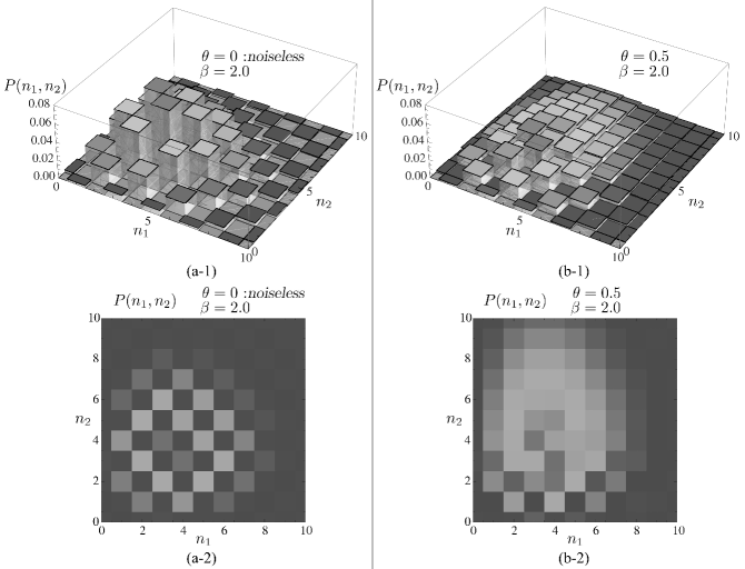
Figure 1: Photon-number distribution P(n1,n2)𝑃subscript𝑛1subscript𝑛2P(n_{1},n_{2}) of the state 𝚽2subscript𝚽2\boldsymbol{\Phi}_{2}. (a-1) P(n1,n2)𝑃subscript𝑛1subscript𝑛2P(n_{1},n_{2}) for θ=0𝜃0\theta=0 and β=2.0𝛽2.0\beta=2.0. (a-2) Contour plot of (a-1). (b-1) P(n1,n2)𝑃subscript𝑛1subscript𝑛2P(n_{1},n_{2}) for θ=0.5𝜃0.5\theta=0.5 and β=2.0𝛽2.0\beta=2.0. (b-2) Contour plot of (b-1).

where

g1(β,k1)subscript𝑔1superscript𝛽subscript𝑘1\displaystyle g_{1}(\beta^{\prime},k_{1}) =\displaystyle= k1|β11=exp[|β|22]βk1k1!,\displaystyle{}_{1}\langle{k_{1}}|{\beta^{\prime}}\rangle_{1}=\exp[-\frac{|\beta^{\prime}|^{2}}{2}]\frac{\beta^{\prime k_{1}}}{\sqrt{{k_{1}}!}}, (30)
g23(β,k2,k3)subscript𝑔23superscript𝛽subscript𝑘2subscript𝑘3\displaystyle g_{23}(\beta^{\prime},k_{2},k_{3}) =\displaystyle= k2,k3|𝐓^23(θ)|β,0~2323\displaystyle{}_{23}\langle{k_{2},k_{3}}|\hat{\bf T}_{23}(\theta)|{\beta^{\prime},\tilde{0}}\rangle_{23} (34)
=\displaystyle= {1coshθexp[12|β|2]k3!k2!(k2k3)βk2k3(sinhθ)k3(coshθ)k2,if k2k30,if k2<k3cases1𝜃12superscriptsuperscript𝛽2subscript𝑘3subscript𝑘2binomialsubscript𝑘2subscript𝑘3superscript𝛽subscript𝑘2subscript𝑘3superscript𝜃subscript𝑘3superscript𝜃subscript𝑘2if subscript𝑘2subscript𝑘3missing-subexpressionmissing-subexpression0if subscript𝑘2subscript𝑘3\displaystyle\left\{\begin{array}[]{rl}\displaystyle\frac{1}{\cosh\theta}\exp[-\frac{1}{2}|\beta^{\prime}|^{2}]\sqrt{\frac{k_{3}!}{k_{2}!}}{k_{2}\choose k_{3}}\beta^{\prime k_{2}-k_{3}}\frac{(\sinh\theta)^{k_{3}}}{(\cosh\theta)^{k_{2}}},&\mbox{if }k_{2}\geq k_{3}\\ &\\ 0,&\mbox{if }k_{2}<k_{3}\end{array}\right.

and we have applied the calculation result of Ref. 24 to obtain Eq.(34). From Eqs.(26)-(29), the photon-number distributions P(n1,n2)=n1,n2|𝝆^12(𝚽i)|n1,n2𝑃subscript𝑛1subscript𝑛2quantum-operator-productsubscript𝑛1subscript𝑛2subscript^𝝆12subscript𝚽𝑖subscript𝑛1subscript𝑛2P(n_{1},n_{2})=\langle{n_{1},n_{2}}|\hat{\boldsymbol{\rho}}_{12}(\boldsymbol{\Phi}_{i})|{n_{1},n_{2}}\rangle can be derived. Figure 1 shows examples of photon-number distribution P(n1,n2)𝑃subscript𝑛1subscript𝑛2P(n_{1},n_{2}) of the state 𝚽2subscript𝚽2\boldsymbol{\Phi}_{2} for β=2.0𝛽2.0\beta=2.0. The graphs (a-1) and (a-2) show the case of θ=0𝜃0\theta=0, that is, noiseless case, and the graphs (b-1) and (b-2) show the case of θ=0.5𝜃0.5\theta=0.5. When there is no thermal noise (θ=0𝜃0\theta=0), the distribution P(n1,n2)𝑃subscript𝑛1subscript𝑛2P(n_{1},n_{2}) is not equal to zero only if n1+n2subscript𝑛1subscript𝑛2n_{1}+n_{2} is odd. From this fact, |𝚽212subscriptketsubscript𝚽212|{\boldsymbol{\Phi}_{2}}\rangle_{12} is understood as the odd two-mode coherent state [25]. On the other hand, we see that this property is destroyed due to the effect of thermal noise from the case of θ=0.5𝜃0.5\theta=0.5, in which the dispersion of the photon-number distribution is appeared in the direction of the n2subscript𝑛2n_{2}-axis.

4 Evaluation of the degree of entanglement of 𝚽2subscript𝚽2\boldsymbol{\Phi}_{2}

As mentioned in Section 2, the states 𝚽2subscript𝚽2\boldsymbol{\Phi}_{2} and 𝚽4subscript𝚽4\boldsymbol{\Phi}_{4} are maximally entangled when there is no noise (Eq.(13)). Further, these two states are associated with each other by a unitary operator (Eq.(6)). In this section, we consider the entanglement property of the state 𝚽2subscript𝚽2\boldsymbol{\Phi}_{2} with thermal noise. The analysis method of the entanglement property of 𝝆^12(𝚽2)subscript^𝝆12subscript𝚽2\hat{\boldsymbol{\rho}}_{12}(\boldsymbol{\Phi}_{2}) is based on Ref. 26.

The fully entangled fraction for the state 𝝈^12subscript^𝝈12\hat{\boldsymbol{\sigma}}_{12} is defined as

f(𝝈^12)=max𝐞|𝝈^12|𝐞1212,f(\hat{\boldsymbol{\sigma}}_{12})=\max{}_{12}\langle{\bf e}|\hat{\boldsymbol{\sigma}}_{12}|{\bf e}\rangle_{12}, (35)

where the maximum is taken over all maximally entangled states |𝐞12subscriptket𝐞12|{\bf e}\rangle_{12}. Here we let

f(𝝆^12(𝚽2))=maxα[𝚽2(α)|𝝆^12(𝚽2)|𝚽2(α)1212],f(\hat{\boldsymbol{\rho}}_{12}(\boldsymbol{\Phi}_{2}))=\max_{\alpha}\Bigl{[}{}_{12}\langle{\boldsymbol{\Phi}_{2}(\alpha)}|\hat{\boldsymbol{\rho}}_{12}(\boldsymbol{\Phi}_{2})|{\boldsymbol{\Phi}_{2}(\alpha)}\rangle_{12}\Bigr{]}, (36)

in order to analyse the state 𝝆^12(𝚽2)subscript^𝝆12subscript𝚽2\hat{\boldsymbol{\rho}}_{12}(\boldsymbol{\Phi}_{2}). Note that we chose the state |𝚽2(α)12=𝒩(α)[|α,α12|α,α12]subscriptketsubscript𝚽2𝛼12subscript𝒩𝛼delimited-[]subscriptket𝛼𝛼12subscriptket𝛼𝛼12{|{\boldsymbol{\Phi}_{2}(\alpha)}\rangle_{12}}={\mathcal{N}_{-}(\alpha)\left[|{\alpha,\alpha}\rangle_{12}-|{-\alpha,-\alpha}\rangle_{12}\right]} as a maximally entangled state, where 𝒩(α)=1/2(1exp[4|α|2])subscript𝒩𝛼1214superscript𝛼2\mathcal{N}_{-}(\alpha)=1/\sqrt{2(1-\exp[-4|\alpha|^{2}])}. The complete form of Eq.(36) is shown in Appendix A. By using the resulting value of f(𝝆^12(𝚽2))𝑓subscript^𝝆12subscript𝚽2f(\hat{\boldsymbol{\rho}}_{12}(\boldsymbol{\Phi}_{2})), a lower bound of the entanglement of formation is given by

E(𝝆^12(𝚽2))𝖧(f(𝝆^12(𝚽2))),𝐸subscript^𝝆12subscript𝚽2𝖧𝑓subscript^𝝆12subscript𝚽2E(\hat{\boldsymbol{\rho}}_{12}(\boldsymbol{\Phi}_{2}))\geq{\sf H}(f(\hat{\boldsymbol{\rho}}_{12}(\boldsymbol{\Phi}_{2}))), (37)

where

𝖧(f)={h2(12+f(1f)),f0.50,f<0.5𝖧𝑓casessubscript212𝑓1𝑓𝑓0.50𝑓0.5{\sf H}(f)=\left\{\begin{array}[]{rl}h_{2}(\frac{1}{2}+\sqrt{f(1-f)}),&f\geq 0.5\\ 0,&f<0.5\end{array}\right. (38)

with the binary entropy function h2(x)=xlog2x(1x)log2(1x)subscript2𝑥𝑥subscript2𝑥1𝑥subscript21𝑥h_{2}(x)=-x\log_{2}x-(1-x)\log_{2}(1-x).

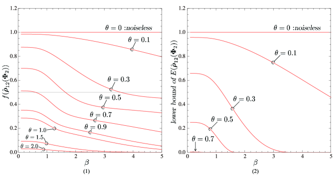
Figure 2 shows the numerical behavior of f(𝝆^12(𝚽2))𝑓subscript^𝝆12subscript𝚽2f(\hat{\boldsymbol{\rho}}_{12}(\boldsymbol{\Phi}_{2})) and the lower bound of E(𝝆^12(𝚽2))𝐸subscript^𝝆12subscript𝚽2E(\hat{\boldsymbol{\rho}}_{12}(\boldsymbol{\Phi}_{2})) obtained from the value of f(𝝆^12(𝚽2))𝑓subscript^𝝆12subscript𝚽2f(\hat{\boldsymbol{\rho}}_{12}(\boldsymbol{\Phi}_{2})). Although it might not be tight, the degradation of the degree of entanglement due to thermal noise is obviously observed through the graph (2) of Figure 2. Thus the degree of entanglement is degraded by increasing the amplitude parameter β𝛽\beta and by increasing the thermal noise parameter θ𝜃\theta. The threshold level of f𝑓f in the function 𝖧(f)𝖧𝑓{\sf H}(f) is 0.50.50.5. Hence, from the graph (1) of Figure 2, we roughly estimate that the limit of the thermal noise parameter θ𝜃\theta to keep entanglement is 0.7similar-toabsent0.7\sim 0.7.

Refer to caption

Figure 2: Entanglement property. (1) behavior of f(𝝆^12(𝚽2))𝑓subscript^𝝆12subscript𝚽2f(\hat{\boldsymbol{\rho}}_{12}(\boldsymbol{\Phi}_{2})). (2) lower bound of E(𝝆^12(𝚽2))𝐸subscript^𝝆12subscript𝚽2E(\hat{\boldsymbol{\rho}}_{12}(\boldsymbol{\Phi}_{2})) obtained from f(𝝆^12(𝚽2))𝑓subscript^𝝆12subscript𝚽2f(\hat{\boldsymbol{\rho}}_{12}(\boldsymbol{\Phi}_{2})).


5 Error performance in the minimax discrimination problem

Suppose there are two quantum states σ^𝟢subscript^𝜎0\hat{\sigma}_{\sf 0} and σ^𝟣subscript^𝜎1\hat{\sigma}_{\sf 1}, where σ^i0subscript^𝜎𝑖0\hat{\sigma}_{i}\geq 0 and Trσ^i=1Trsubscript^𝜎𝑖1{\rm Tr}\hat{\sigma}_{i}=1. If the probability distribution 𝐩=(p𝟢,p𝟣)𝐩subscript𝑝0subscript𝑝1{\bf p}=(p_{\sf 0},p_{\sf 1}) of the states is given in advance, one can employ the quantum Bayes strategy [27, 28]. At that time, the average probability of error of the Bayes optimal discrimination for given 𝐩𝐩{\bf p} is formally written as

P¯emin(𝐩)=minΠ[p𝟢TrΠ^𝟣σ^𝟢+p𝟣TrΠ^𝟢σ^𝟣],superscriptsubscript¯𝑃emin𝐩subscriptΠsubscript𝑝0Trsubscript^Π1subscript^𝜎0subscript𝑝1Trsubscript^Π0subscript^𝜎1\bar{P}_{\rm e}^{\rm min}({\bf p})=\min_{\mit\Pi}\left[p_{\sf 0}{\rm Tr}\hat{\mit\Pi}_{\sf 1}\hat{\sigma}_{\sf 0}+p_{\sf 1}{\rm Tr}\hat{\mit\Pi}_{\sf 0}\hat{\sigma}_{\sf 1}\right], (39)

where Π={Π^𝟢,Π^𝟣:Π^𝟢+Π^𝟣=1^andΠ^i0}Πconditional-setsubscript^Π0subscript^Π1subscript^Π0subscript^Π1^1andsubscript^Π𝑖0{\mit\Pi}=\{\hat{\mit\Pi}_{\sf 0},\hat{\mit\Pi}_{\sf 1}:\hat{\mit\Pi}_{\sf 0}+\hat{\mit\Pi}_{\sf 1}=\hat{1}\ {\rm and}\ \hat{\mit\Pi}_{i}\geq 0\} is a positive operator-valued measure (POVM) which describes a detection profile for the states.

Clearly P¯emin(𝐩)superscriptsubscript¯𝑃emin𝐩\bar{P}_{\rm e}^{\rm min}({\bf p}) depends on the choice of 𝐩𝐩\bf p. To remove the dependency of choice of the probability distribution 𝐩𝐩\bf p, we employ the quantum minimax strategy [10, 11, 12]. When the quantum minimax strategy is employed, the average probability of error in the minimax optimal discrimination is given by

P¯e=minΠmax𝐩[p𝟢TrΠ^𝟣σ^𝟢+p𝟣TrΠ^𝟢σ^𝟣]=max𝐩minΠ[p𝟢TrΠ^𝟣σ^𝟢+p𝟣TrΠ^𝟢σ^𝟣]=max𝐩[P¯emin(𝐩)].superscriptsubscript¯𝑃esubscriptΠsubscript𝐩subscript𝑝0Trsubscript^Π1subscript^𝜎0subscript𝑝1Trsubscript^Π0subscript^𝜎1subscript𝐩subscriptΠsubscript𝑝0Trsubscript^Π1subscript^𝜎0subscript𝑝1Trsubscript^Π0subscript^𝜎1subscript𝐩superscriptsubscript¯𝑃emin𝐩\bar{P}_{\rm e}^{\circ}=\min_{\mit\Pi}\max_{\bf p}\left[p_{\sf 0}{\rm Tr}\hat{\mit\Pi}_{\sf 1}\hat{\sigma}_{\sf 0}+p_{\sf 1}{\rm Tr}\hat{\mit\Pi}_{\sf 0}\hat{\sigma}_{\sf 1}\right]=\max_{\bf p}\min_{\mit\Pi}\left[p_{\sf 0}{\rm Tr}\hat{\mit\Pi}_{\sf 1}\hat{\sigma}_{\sf 0}+p_{\sf 1}{\rm Tr}\hat{\mit\Pi}_{\sf 0}\hat{\sigma}_{\sf 1}\right]=\max_{\bf p}\left[\bar{P}_{\rm e}^{\rm min}({\bf p})\right]. (40)

It is not easy to find the optimal probability distribution 𝐩superscript𝐩{\bf p}^{\circ} in general. However, if the states σ^𝟢subscript^𝜎0\hat{\sigma}_{\sf 0} and σ^𝟣subscript^𝜎1\hat{\sigma}_{\sf 1} are symmetric, the optimal distribution becomes the uniform distribution 𝐮=(1/2,1/2)𝐮1212{\bf u}=(1/2,1/2). At that time, we have P¯e=P¯emin(1/2,1/2)superscriptsubscript¯𝑃esuperscriptsubscript¯𝑃emin1212\bar{P}_{\rm e}^{\circ}=\bar{P}_{\rm e}^{\rm min}(1/2,1/2). Recalling the Helstrom’s algorithm for calculating the minimum error probability for binary states [27], it becomes

P¯e=1212λi0λisuperscriptsubscript¯𝑃e1212subscriptsubscript𝜆𝑖0subscript𝜆𝑖\bar{P}_{\rm e}^{\circ}=\frac{1}{2}-\frac{1}{2}\sum_{\lambda_{i}\geq 0}\lambda_{i} (41)

where λisubscript𝜆𝑖\lambda_{i} are the eigenvalues of σ^𝟢σ^𝟣subscript^𝜎0subscript^𝜎1\hat{{\sigma}}_{\sf 0}-\hat{{\sigma}}_{\sf 1}.

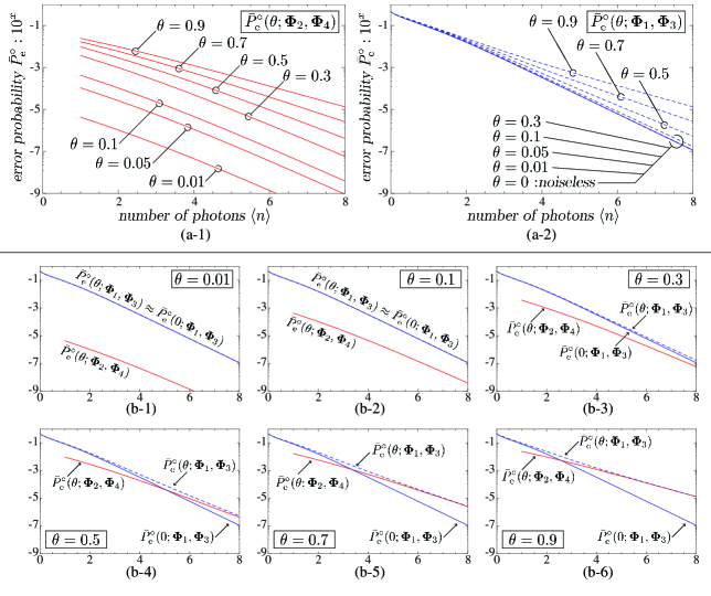
Applying the result of Eq.(41), we can compute the error probabilities for the set of the states 𝚽2subscript𝚽2\boldsymbol{\Phi}_{2} and 𝚽4subscript𝚽4\boldsymbol{\Phi}_{4}, and for the set of 𝚽1subscript𝚽1\boldsymbol{\Phi}_{1} and 𝚽3subscript𝚽3\boldsymbol{\Phi}_{3} in terms of the minimax discrimination problem. Results of the numerical calculation are shown in Figure 3. The graphs (a-1) and (a-2) illustrate P¯e(θ;𝚽2,𝚽4)superscriptsubscript¯𝑃e𝜃subscript𝚽2subscript𝚽4\bar{P}_{\rm e}^{\circ}(\theta;\boldsymbol{\Phi}_{2},\boldsymbol{\Phi}_{4}) and P¯e(θ;𝚽1,𝚽3)superscriptsubscript¯𝑃e𝜃subscript𝚽1subscript𝚽3\bar{P}_{\rm e}^{\circ}(\theta;\boldsymbol{\Phi}_{1},\boldsymbol{\Phi}_{3}), respectively, for θ=0.01,0.05,0.1,0.3,0.5,0.7𝜃0.010.050.10.30.50.7\theta=0.01,0.05,0.1,0.3,0.5,0.7, and 0.90.90.9. Comparing these two graphs, it is noticed that the behavior of P¯e(θ;𝚽2,𝚽4)superscriptsubscript¯𝑃e𝜃subscript𝚽2subscript𝚽4\bar{P}_{\rm e}^{\circ}(\theta;\boldsymbol{\Phi}_{2},\boldsymbol{\Phi}_{4}) is different from that of P¯e(θ;𝚽1,𝚽3)superscriptsubscript¯𝑃e𝜃subscript𝚽1subscript𝚽3\bar{P}_{\rm e}^{\circ}(\theta;\boldsymbol{\Phi}_{1},\boldsymbol{\Phi}_{3}). Recall that P¯e(θ;𝚽2,𝚽4)=0superscriptsubscript¯𝑃e𝜃subscript𝚽2subscript𝚽40\bar{P}_{\rm e}^{\circ}(\theta;\boldsymbol{\Phi}_{2},\boldsymbol{\Phi}_{4})=0 if θ=0𝜃0\theta=0. As a value of the thermal noise parameter θ𝜃\theta increases, the error probability P¯e(θ;𝚽2,𝚽4)superscriptsubscript¯𝑃e𝜃subscript𝚽2subscript𝚽4\bar{P}_{\rm e}^{\circ}(\theta;\boldsymbol{\Phi}_{2},\boldsymbol{\Phi}_{4}) rapidly moves upward, while the error probability P¯e(θ;𝚽1,𝚽3)superscriptsubscript¯𝑃e𝜃subscript𝚽1subscript𝚽3\bar{P}_{\rm e}^{\circ}(\theta;\boldsymbol{\Phi}_{1},\boldsymbol{\Phi}_{3}) changes moderately as if to be the case of binary single-mode coherent states {|β1,|β1}subscriptket𝛽1subscriptket𝛽1\{|{\beta}\rangle_{1},|{-\beta}\rangle_{1}\}. The graphs (b-1) to (b-6) involve numerical comparison between P¯e(θ;𝚽2,𝚽4)superscriptsubscript¯𝑃e𝜃subscript𝚽2subscript𝚽4\bar{P}_{\rm e}^{\circ}(\theta;\boldsymbol{\Phi}_{2},\boldsymbol{\Phi}_{4}) and P¯e(θ;𝚽1,𝚽3)superscriptsubscript¯𝑃e𝜃subscript𝚽1subscript𝚽3\bar{P}_{\rm e}^{\circ}(\theta;\boldsymbol{\Phi}_{1},\boldsymbol{\Phi}_{3}) for each θ𝜃\theta. In all cases from (b-1) to (b-6), P¯e(θ;𝚽2,𝚽4)superscriptsubscript¯𝑃e𝜃subscript𝚽2subscript𝚽4\bar{P}_{\rm e}^{\circ}(\theta;\boldsymbol{\Phi}_{2},\boldsymbol{\Phi}_{4}) is always smaller than P¯e(θ;𝚽1,𝚽3)superscriptsubscript¯𝑃e𝜃subscript𝚽1subscript𝚽3\bar{P}_{\rm e}^{\circ}(\theta;\boldsymbol{\Phi}_{1},\boldsymbol{\Phi}_{3}). But, the gap between P¯e(θ;𝚽2,𝚽4)superscriptsubscript¯𝑃e𝜃subscript𝚽2subscript𝚽4\bar{P}_{\rm e}^{\circ}(\theta;\boldsymbol{\Phi}_{2},\boldsymbol{\Phi}_{4}) and P¯e(θ;𝚽1,𝚽3)superscriptsubscript¯𝑃e𝜃subscript𝚽1subscript𝚽3\bar{P}_{\rm e}^{\circ}(\theta;\boldsymbol{\Phi}_{1},\boldsymbol{\Phi}_{3}) is getting smaller when the thermal noise parameter θ𝜃\theta increases. When θ𝜃\theta is small enough (θ0.1similar-to𝜃0.1\theta\sim 0.1 or less), one can easily find a clear gap between P¯e(θ;𝚽2,𝚽4)superscriptsubscript¯𝑃e𝜃subscript𝚽2subscript𝚽4\bar{P}_{\rm e}^{\circ}(\theta;\boldsymbol{\Phi}_{2},\boldsymbol{\Phi}_{4}) and P¯e(θ;𝚽1,𝚽3)superscriptsubscript¯𝑃e𝜃subscript𝚽1subscript𝚽3\bar{P}_{\rm e}^{\circ}(\theta;\boldsymbol{\Phi}_{1},\boldsymbol{\Phi}_{3}) in the region 0n8similar-to0delimited-⟨⟩𝑛similar-to80\sim\langle n\rangle\sim 8. When θ𝜃\theta increases, P¯e(θ;𝚽2,𝚽4)superscriptsubscript¯𝑃e𝜃subscript𝚽2subscript𝚽4\bar{P}_{\rm e}^{\circ}(\theta;\boldsymbol{\Phi}_{2},\boldsymbol{\Phi}_{4}) approaches to P¯e(θ;𝚽1,𝚽3)superscriptsubscript¯𝑃e𝜃subscript𝚽1subscript𝚽3\bar{P}_{\rm e}^{\circ}(\theta;\boldsymbol{\Phi}_{1},\boldsymbol{\Phi}_{3}), and finally P¯e(θ;𝚽2,𝚽4)superscriptsubscript¯𝑃e𝜃subscript𝚽2subscript𝚽4\bar{P}_{\rm e}^{\circ}(\theta;\boldsymbol{\Phi}_{2},\boldsymbol{\Phi}_{4}) almost touches to P¯e(θ;𝚽1,𝚽3)superscriptsubscript¯𝑃e𝜃subscript𝚽1subscript𝚽3\bar{P}_{\rm e}^{\circ}(\theta;\boldsymbol{\Phi}_{1},\boldsymbol{\Phi}_{3}).

Refer to caption

Figure 3: Error performance. (a-1) P¯e(θ;𝚽2,𝚽4)superscriptsubscript¯𝑃e𝜃subscript𝚽2subscript𝚽4\bar{P}_{\rm e}^{\circ}(\theta;\boldsymbol{\Phi}_{2},\boldsymbol{\Phi}_{4}) for θ=0.01,0.05,0.1,0.3,0.5,0.7𝜃0.010.050.10.30.50.7\theta=0.01,0.05,0.1,0.3,0.5,0.7, and 0.90.90.9. (a-2) P¯e(θ;𝚽1,𝚽3)superscriptsubscript¯𝑃e𝜃subscript𝚽1subscript𝚽3\bar{P}_{\rm e}^{\circ}(\theta;\boldsymbol{\Phi}_{1},\boldsymbol{\Phi}_{3}) for θ=0,0.01,0.05,0.1,0.3,0.5,0.7𝜃00.010.050.10.30.50.7\theta=0,0.01,0.05,0.1,0.3,0.5,0.7, and 0.90.90.9. (b-1) P¯e(θ;𝚽2,𝚽4)superscriptsubscript¯𝑃e𝜃subscript𝚽2subscript𝚽4\bar{P}_{\rm e}^{\circ}(\theta;\boldsymbol{\Phi}_{2},\boldsymbol{\Phi}_{4}) vs P¯e(θ;𝚽1,𝚽3)superscriptsubscript¯𝑃e𝜃subscript𝚽1subscript𝚽3\bar{P}_{\rm e}^{\circ}(\theta;\boldsymbol{\Phi}_{1},\boldsymbol{\Phi}_{3}) at θ=0.01𝜃0.01\theta=0.01. (b-2) P¯e(θ;𝚽2,𝚽4)superscriptsubscript¯𝑃e𝜃subscript𝚽2subscript𝚽4\bar{P}_{\rm e}^{\circ}(\theta;\boldsymbol{\Phi}_{2},\boldsymbol{\Phi}_{4}) vs P¯e(θ;𝚽1,𝚽3)superscriptsubscript¯𝑃e𝜃subscript𝚽1subscript𝚽3\bar{P}_{\rm e}^{\circ}(\theta;\boldsymbol{\Phi}_{1},\boldsymbol{\Phi}_{3}) at θ=0.1𝜃0.1\theta=0.1. (b-3) P¯e(θ;𝚽2,𝚽4)superscriptsubscript¯𝑃e𝜃subscript𝚽2subscript𝚽4\bar{P}_{\rm e}^{\circ}(\theta;\boldsymbol{\Phi}_{2},\boldsymbol{\Phi}_{4}) vs P¯e(θ;𝚽1,𝚽3)superscriptsubscript¯𝑃e𝜃subscript𝚽1subscript𝚽3\bar{P}_{\rm e}^{\circ}(\theta;\boldsymbol{\Phi}_{1},\boldsymbol{\Phi}_{3}) at θ=0.3𝜃0.3\theta=0.3. (b-4) P¯e(θ;𝚽2,𝚽4)superscriptsubscript¯𝑃e𝜃subscript𝚽2subscript𝚽4\bar{P}_{\rm e}^{\circ}(\theta;\boldsymbol{\Phi}_{2},\boldsymbol{\Phi}_{4}) vs P¯e(θ;𝚽1,𝚽3)superscriptsubscript¯𝑃e𝜃subscript𝚽1subscript𝚽3\bar{P}_{\rm e}^{\circ}(\theta;\boldsymbol{\Phi}_{1},\boldsymbol{\Phi}_{3}) at θ=0.5𝜃0.5\theta=0.5. (b-5) P¯e(θ;𝚽2,𝚽4)superscriptsubscript¯𝑃e𝜃subscript𝚽2subscript𝚽4\bar{P}_{\rm e}^{\circ}(\theta;\boldsymbol{\Phi}_{2},\boldsymbol{\Phi}_{4}) vs P¯e(θ;𝚽1,𝚽3)superscriptsubscript¯𝑃e𝜃subscript𝚽1subscript𝚽3\bar{P}_{\rm e}^{\circ}(\theta;\boldsymbol{\Phi}_{1},\boldsymbol{\Phi}_{3}) at θ=0.7𝜃0.7\theta=0.7. (b-6) P¯e(θ;𝚽2,𝚽4)superscriptsubscript¯𝑃e𝜃subscript𝚽2subscript𝚽4\bar{P}_{\rm e}^{\circ}(\theta;\boldsymbol{\Phi}_{2},\boldsymbol{\Phi}_{4}) vs P¯e(θ;𝚽1,𝚽3)superscriptsubscript¯𝑃e𝜃subscript𝚽1subscript𝚽3\bar{P}_{\rm e}^{\circ}(\theta;\boldsymbol{\Phi}_{1},\boldsymbol{\Phi}_{3}) at θ=0.9𝜃0.9\theta=0.9.


5.1 Conclusions

The so-called quasi-Bell entangled coherent states, 𝚽1subscript𝚽1\boldsymbol{\Phi}_{1}, 𝚽2subscript𝚽2\boldsymbol{\Phi}_{2}, 𝚽3subscript𝚽3\boldsymbol{\Phi}_{3} and 𝚽4subscript𝚽4\boldsymbol{\Phi}_{4}, were studied in the presence of thermal noise. In the analysis, we assumed thermal noise affects only one of the two modes of each state. By using the thermalizing operator with thermal noise parameter θ𝜃\theta, the matrix representation of the density operators of the quasi-Bell entangled coherent states with thermal noise was derived. To seek the entanglement property of the states in the presence of thermal noise, a lower bound of the entanglement of formation for the state 𝚽2subscript𝚽2\boldsymbol{\Phi}_{2} was numerically computed. From this, we observed that the range of θ𝜃\theta to keep entanglement of 𝚽2subscript𝚽2\boldsymbol{\Phi}_{2} is limited to a small region. We also considered the optimal quantum discrimination problem for the states 𝚽2subscript𝚽2\boldsymbol{\Phi}_{2} and 𝚽4subscript𝚽4\boldsymbol{\Phi}_{4} and for 𝚽1subscript𝚽1\boldsymbol{\Phi}_{1} and 𝚽3subscript𝚽3\boldsymbol{\Phi}_{3}. From numerical comparison, it is noticed that the behavior of the error probability P¯e(θ;𝚽2,𝚽4)superscriptsubscript¯𝑃e𝜃subscript𝚽2subscript𝚽4\bar{P}_{\rm e}^{\circ}(\theta;\boldsymbol{\Phi}_{2},\boldsymbol{\Phi}_{4}) is different from that of P¯e(θ;𝚽1,𝚽3)superscriptsubscript¯𝑃e𝜃subscript𝚽1subscript𝚽3\bar{P}_{\rm e}^{\circ}(\theta;\boldsymbol{\Phi}_{1},\boldsymbol{\Phi}_{3}), and the gap between P¯e(θ;𝚽2,𝚽4)superscriptsubscript¯𝑃e𝜃subscript𝚽2subscript𝚽4\bar{P}_{\rm e}^{\circ}(\theta;\boldsymbol{\Phi}_{2},\boldsymbol{\Phi}_{4}) and P¯e(θ;𝚽1,𝚽3)superscriptsubscript¯𝑃e𝜃subscript𝚽1subscript𝚽3\bar{P}_{\rm e}^{\circ}(\theta;\boldsymbol{\Phi}_{1},\boldsymbol{\Phi}_{3}) is getting smaller when θ𝜃\theta increases. The advantage of the use of the states of 𝚽2subscript𝚽2\boldsymbol{\Phi}_{2} and 𝚽4subscript𝚽4\boldsymbol{\Phi}_{4} against the states of 𝚽1subscript𝚽1\boldsymbol{\Phi}_{1} and 𝚽3subscript𝚽3\boldsymbol{\Phi}_{3} vanishes when θ𝜃\theta is large. In summary, the effective range for the use of the states of 𝚽2subscript𝚽2\boldsymbol{\Phi}_{2} and 𝚽4subscript𝚽4\boldsymbol{\Phi}_{4} in information-communication applications would be limited rather than other two, so that careful design for such applications is needed.

acknowledgment

The author is grateful to Professor Osamu Hirota of Tamagawa University for his helpful discussions. This work was supported in part by JSPS KAKENHI Grant Number 15K06082.

References

  • [1] Sanders, B.C., “Review of entangled coherent states,” J. Phys. A: Math. Theor. 45(24), 244002 (2012).
  • [2] Sanders, B.C, “Forty-five years of entangled coherent states,” Proceedings of the first international workshop on entangled coherent states and its application to quantum information science (Edited by Usuda, T.S. and Kato, K.), 111-113 (2013).
  • [3] Hirota, O. and Sasaki, M., “Entangled state based on nonorthogonal state,” Proc. QCM&C-Y2K (Edited by Tombeshi, P. and Hirota, O.), 359-366 (2001).
  • [4] van Enk, S.J. and Hirota, O., “Entangled coherent states: Teleportation and decoherence,” Phys. Rev. A 64(2), 022313 (2001).
  • [5] Wang, X., “Quantum teleportation of entangled coherent states,” Phys. Rev. A 64(2), 022302 (2001).
  • [6] Jeong, H., Kim, M.S. and Lee, J., “Quantum-information processing for a coherent superposition state via a mixed entangled coherent channel,” Phys. Rev. A 64(5), 052308 (2001).
  • [7] Jeong, H. and Kim, M.S., “Efficient quantum computation using coherent states,” Phys. Rev. A 65(4), 042305 (2002).
  • [8] Hirota, O., “Error free quantum reading by quasi Bell state of entangled coherent states,” e-print arXiv:quant-ph/1108.4163v2 (2011).
  • [9] Kato, K. and Hirota,O., “Effect of decoherence in quantum reading with phase shift keying signal of entangled coherent states,” Proc. SPIE 8875, 88750P(2013).
  • [10] Hirota, O. and Ikehara, S., “Minimax strategy in the quantum detection theory and its application to optical communications,” Trans. IECE of Japan E65, 627-633 (1982).
  • [11] Kato, K., “Necessary and sufficient conditions for minimax strategy in quantum signal detection,” 2012 IEEE Int. Sympo. Inform. Theory (ISIT) Proc., 1082-1086 (2012).
  • [12] Nakahira, K., Kato, K. and Usuda, T.S., “Generalized quantum state discrimination problems,” Phys. Rev. A 91(5), 052304 (2015).
  • [13] Barnett, S.M. and Phoenix, S.J., “Entropy as a measure of quantum optical correlation,” Phys. Rev. A 40, 2404-2409 (1989).
  • [14] Bennett, C.H., Bernstein, H.J., Popescu, S. and Schumacher, B., “Concentrating partial entanglement by local operations,” Phys. Rev. A 53, 2046-2052 (1996).
  • [15] Takahashi, Y. and Umezawa, H., “Thermo field dynamics,” Collect. Phenom. 2, 55-80 (1975).
  • [16] Barnett, S.M. and Knight, P.L., “Thermofield analysis of squeezing and statistical mixtures in quantum optics,” J. Opt. Soc. Am. B, 2(3), 467-479 (1985).
  • [17] Fearn, H. and Collett M.J., “Representation of squeezed states with thermal noise,” J. Mod. Opt. 35(3), 553-564 (1988).
  • [18] Mann, A. and Revzen, M., “Thermal coherent states,” Phys. Lett. A 134(5), 273-275 (1989).
  • [19] Oz-Vogt, J., Mann, A. and Revzen, M., “Thermal coherent states and thermal squeezed states,” J. Mod. Opt. 38(12), 2339-2347 (1991).
  • [20] Kireev, A., Mann, A., Revzen, M. and Umezawa, H., “Thermal squeezed states in thermo field dynamics and quantum and thermal fluctuations,” Phys. Lett. A 142(4/5), 215-221 (1989).
  • [21] Lee, C.T., “Two-mode squeezed states with thermal noise,” Phys. Rev. A 42(7), 4193-4198 (1990).
  • [22] Lu, W.F., “Thermalized displaced and squeezed number states in the coordinate representation,” J. Phys. A: Math. Gen. 32(27), 5037 (1999).
  • [23] Lu, W.F., “Thermalized displaced squeezed thermal states,” J. Phys. A: Math. Gen. 33(3), 479 (2000).
  • [24] Selvadoray, M., Kumar, M.S. and Simon, R., “Photon distribution in two-mode squeezed coherent states with complex displacement and squeeze parameters,” Phys. Rev. A, 49(6), 4957-4967 (1994).
  • [25] Chai, C.L., “Two-mode nonclassical state via superpositions of two-mode coherent states,” Phys. Rev. A 46(11), 7187-7191 (1992).
  • [26] Hirota, O., van Enk, S.J., Nakamura, K., Sohma, M. and Kato, K., “Entangled nonorthogonal states and their decoherence properties,” e-print arXiv:quant-ph/0101096v1 (2001).
  • [27] Helstrom, C. W., Quantum Detection and Estimation Theory, Academic Press, New York, (1976).
  • [28] Holevo, A.S., Statistical Structure of Quantum Theory, Springer, Berlin, (2001).

Appendix A

Eq.(36) is given by

f(𝝆^12(𝚽2))=maxα[[\displaystyle f(\hat{\boldsymbol{\rho}}_{12}(\boldsymbol{\Phi}_{2}))=\max_{\alpha}\Bigl{[}\Bigl{[} 2𝒩2(α)𝒩2(β)cosh2θ×{\displaystyle 2\frac{\mathcal{N}_{-}^{2}(\alpha)\mathcal{N}_{-}^{2}(\beta)}{\cosh^{2}\theta}\times\Bigl{\{}
+exp[|αcoshθβ|2]exp[|αβ|2]superscript𝛼𝜃𝛽2superscript𝛼𝛽2\displaystyle+\exp[-\left|\frac{\alpha}{\cosh\theta}-\beta\right|^{2}]\exp[-|\alpha-\beta|^{2}]
exp[|α|2(1+tanh2θ)+αβcoshθαβcoshθ|β|2]exp[|α|2+αβαβ|β|2]superscript𝛼21superscript2𝜃superscript𝛼𝛽𝜃𝛼superscript𝛽𝜃superscript𝛽2superscript𝛼2superscript𝛼𝛽𝛼superscript𝛽superscript𝛽2\displaystyle-\exp[-|\alpha|^{2}(1+\tanh^{2}\theta)+\frac{\alpha^{\ast}\beta}{\cosh\theta}-\frac{\alpha\beta^{\ast}}{\cosh\theta}-|\beta|^{2}]\exp[-|\alpha|^{2}+\alpha^{\ast}\beta-\alpha\beta^{\ast}-|\beta|^{2}]
exp[|α|2(1+tanh2θ)αβcoshθ+αβcoshθ|β|2]exp[|α|2αβ+αβ|β|2]superscript𝛼21superscript2𝜃superscript𝛼𝛽𝜃𝛼superscript𝛽𝜃superscript𝛽2superscript𝛼2superscript𝛼𝛽𝛼superscript𝛽superscript𝛽2\displaystyle-\exp[-|\alpha|^{2}(1+\tanh^{2}\theta)-\frac{\alpha^{\ast}\beta}{\cosh\theta}+\frac{\alpha\beta^{\ast}}{\cosh\theta}-|\beta|^{2}]\exp[-|\alpha|^{2}-\alpha^{\ast}\beta+\alpha\beta^{\ast}-|\beta|^{2}]
+exp[|αcoshθ+β|2]exp[|α+β|2]superscript𝛼𝜃𝛽2superscript𝛼𝛽2\displaystyle+\exp[-\left|\frac{\alpha}{\cosh\theta}+\beta\right|^{2}]\exp[-|\alpha+\beta|^{2}]
exp[|α|21cosh2θ+αβcoshθαβcoshθ|β|2]exp[|α|2+αβαβ|β|2]superscript𝛼21superscript2𝜃superscript𝛼𝛽𝜃𝛼superscript𝛽𝜃superscript𝛽2superscript𝛼2superscript𝛼𝛽𝛼superscript𝛽superscript𝛽2\displaystyle-\exp[-|\alpha|^{2}\frac{1}{\cosh^{2}\theta}+\frac{\alpha^{\ast}\beta}{\cosh\theta}-\frac{\alpha\beta^{\ast}}{\cosh\theta}-|\beta|^{2}]\exp[-|\alpha|^{2}+\alpha^{\ast}\beta-\alpha\beta^{\ast}-|\beta|^{2}]
+exp[|α|2(1+tanh2θ)+αβcoshθ+αβcoshθ|β|2]exp[|αβ|2]superscript𝛼21superscript2𝜃superscript𝛼𝛽𝜃𝛼superscript𝛽𝜃superscript𝛽2superscript𝛼𝛽2\displaystyle+\exp[-|\alpha|^{2}(1+\tanh^{2}\theta)+\frac{\alpha^{\ast}\beta}{\cosh\theta}+\frac{\alpha\beta^{\ast}}{\cosh\theta}-|\beta|^{2}]\exp[-|\alpha-\beta|^{2}]
+exp[|α|2(1+tanh2θ)αβcoshθαβcoshθ|β|2]exp[|α+β|2]superscript𝛼21superscript2𝜃superscript𝛼𝛽𝜃𝛼superscript𝛽𝜃superscript𝛽2superscript𝛼𝛽2\displaystyle+\exp[-|\alpha|^{2}(1+\tanh^{2}\theta)-\frac{\alpha^{\ast}\beta}{\cosh\theta}-\frac{\alpha\beta^{\ast}}{\cosh\theta}-|\beta|^{2}]\exp[-|\alpha+\beta|^{2}]
exp[|α|21cosh2θαβcoshθ+αβcoshθ|β|2]exp[|α|2αβ+αβ|β|2]}]].\displaystyle-\exp[-|\alpha|^{2}\frac{1}{\cosh^{2}\theta}-\frac{\alpha^{\ast}\beta}{\cosh\theta}+\frac{\alpha\beta^{\ast}}{\cosh\theta}-|\beta|^{2}]\exp[-|\alpha|^{2}-\alpha^{\ast}\beta+\alpha\beta^{\ast}-|\beta|^{2}]\Bigr{\}}\quad\Bigr{]}\Bigr{]}.

This maximization problem with respect to α𝛼\alpha was numerically solved to draw the graph (1) of Figure 2 under the restriction that all parameter is real.