On the global convergence of the inexact semi-smooth Newton method for absolute value equation

Abstract

In this paper, we investigate global convergence properties of the inexact nonsmooth Newton method for solving the system of absolute value equations (AVE). Global $Q$-linear convergence is established under suitable assumptions. Moreover, we present some numerical experiments designed to investigate the practical viability of the proposed scheme.

Keywords: Absolute value equation, inexact semi-smooth Newton method, global convergence, numerical experiments.

Mathematical Subject Classification (2010): Primary 90C33; Secondary 15A48.

1 Introduction

Recently, the problem of finding a solution of the system of absolute value equations (AVE)

$$Ax-|x|=b,$$ (1)

where $A\in\mathbb{R}^{n\times n}$ and $b\in\mathbb{R}^{n}\equiv\mathbb{R}^{n\times 1}$, has been received much attention from optimization community. It is currently an active research topic, due to its broad application to many subjects. For instance, linear complementarity problem, linear programming or convex quadratic programming can be equivalently reformulated in the form of (1) and thus solved as absolute value equations; see [12, 17, 8, 19]. As far as we know, since Mangasarian and Meyer [14] established existence results for this class of absolute value equations (1), the interest for this subject has increased substantially; see [13, 11, 20] and reference therein.

Several algorithms have been designed to solve the systems of AVEs involving smooth, semi-smooth and Picard techniques; see [1, 7, 21, 10, 22]. In [9], Mangasarian applied the nonsmooth Newton method for solving AVE obtaining global $Q$-linear convergence and showing its numerical effectiveness. However, each semi-smooth Newton iteration requires the exact solution of a linear system, which has an undesired effect on the computational performance of this method. The exact solution of the linear system, at each iteration of the method, can be computational expensive and may not be justified. A well known alternative is to solve the linear systems involved approximately. A bound for the relative error tolerance to solve subproblem guaranteeing global $Q$-linear convergence will arise very clearly in the present work. Besides, the inexact analysis support the efficient computational implementations of the exact schemes, for this reason they are important and necessaries. Following the ideas of [4] and [9], we use the inexact nonsmooth Newton method for solving absolute value equations and present some computational experiments designed to investigate its practical viability.

The paper is organized as follows. The next subsection presents some notations and preliminaries that will be used throughout the paper. Section 2 devotes the definition of the inexact Newton method and its global $Q$-linear convergence. Section 3 provides an exhaustive discussion of the computational results of the inexact Newton method when it is compared with the exact one. We complete the paper with some conclusion for further study.

1.1 Preliminaries

In this section we present the notations and some auxiliary results used throughout the paper. Let $\mathbb{R}^{n}$ be denote the $n$-dimensional Euclidean space and $\|\cdot\|$ a norm. The $i$-th component of a vector $x\in\mathbb{R}^{n}$ is denoted by $x_{i}$ for every $i=1,\ldots,n$. For $x\in\mathbb{R}^{n}$, $\operatorname{sgn}(x)$ denotes a vector with components equal to $-1$, $0$ or $1$ depending on whether the corresponding component of the vector $x$ is negative, zero or positive. Denote $|x|$ the vectors with $i$-th component equal to $|x^{i}|$. The set of all $n\times n$ matrices with real entries is denoted by $\mathbb{R}^{n\times n}$ and $\mathbb{R}^{n}\equiv\mathbb{R}^{n\times 1}$. The matrix ${\rm Id}$ denotes the $n\times n$ identity matrix. If $x\in\mathbb{R}^{n}$ then $\operatorname{diag}(x)$ will denote an $n\times n$ diagonal matrix with $(i,i)$-th entry equal to $x^{i}$, $i=1,\dots,n$. For an $M\in\mathbb{R}^{n\times n}$ consider the norm defined by $\|M\|:=\max\{\|Mx\|~{}:~{}x\in\mathbb{R}^{n},~{}\|x\|=1\}$. This definition implies

$$\|Mx\|\leq\|M\|\|x\|,\qquad\|L+M\|\leq\|L\|+\|M\|,\qquad\|LM\|\leq\|L\|\|M\|,$$ (2)

for any matrices $L,M\in\mathbb{R}^{n\times n}$ and $x\in\mathbb{R}^{n}$; see, for instance, Chapter 5 of [6]. The next useful result was proved in 2.1.1, page 32 of [15].

Lemma 1 (Banach’s Lemma).

Let $E\in\mathbb{R}^{n\times n}$. If $\|E\|<1$, then the matrix ${\rm Id}-E$ is invertible and $\|[{\rm Id}-E]^{-1}\|\leq 1/\left(1-\|E\|\right).$

We end this section quoting the following result from combination of Lemma 2 of [9] and Proposition 3 of [14], which gives us a sufficient condition for the invertibility of matrix $A-D(x)$ for all $x\in\mathbb{R}^{n}$ and existence of solution for AVE in (1).

Lemma 2.

Assume that the singular values of the matrix $A\in\mathbb{R}^{n\times n}$ exceed $1$. Then the matrix $A-D(x)$ is invertible for all $x\in\mathbb{R}^{n}$. Moreover, AVE in (1) has unique solution for any $b\in\mathbb{R}^{n}$.

The following proposition was proved in Proposition 4 of [14].

Proposition 1.

Assume that $A\in\mathbb{R}^{n\times n}$ is invertible. If $\left\|A^{-1}\right\|<1$ then AVE in (1) has unique solution for any $b\in\mathbb{R}^{n}$.

2 Inexact Semi-smooth Newton Method

The exact semismooth Newton method [18] for finding the zero of the semismooth function

$$F(x):=Ax-|x|-b,$$ (3)

with starting point $x_{0}\in\mathbb{R}^{n}$, is formally defined by

$$F(x_{k})+V_{k}\left(x_{k+1}-x_{k}\right)=0,\qquad V_{k}\in\partial F(x_{k}),\qquad k=0,1,\ldots,$$

where $\partial F(x)$ denotes the Clarke generalized subdiferential of $F$ at $x\in\mathbb{R}^{n}$; see [2]. Letting

$$D(x):=\mbox{diag}(\mbox{sgn}(x)),\qquad x\in\mathbb{R}^{n},$$ (4)

we obtain from (3) that $A-D(x)\in\partial F(x)$. Hence, the exact semi-smooth Newton method for solving the AVE in (1), which was proposed by Mangasarian [9], generates a sequence formally stated as

$$\left[A-D(x_{k})\right]x_{k+1}=b.$$ (5)

To solve (1), following the ideas of [4], we propose an inexact semi-smooth Newton method, starting at $x_{0}\in\mathbb{R}^{n}$ and residual relative error tolerance $\theta\geq 0$, by

$$\left\|\left[A-D(x_{k})\right]x_{k+1}-b\right\|\leq\theta\left\|F(x_{k})\right\|,\qquad k=0,1,\ldots.$$ (6)

Note that, in absence of errors, i.e., $\theta=0$, the above iteration retrieves (5). In the next section we analyze the convergence properties of $\{x_{k}\}$ generated by the inexact semi-smooth Newton method.

2.1 Convergence Analysis

To establish convergence of the sequence $\{x_{k}\}$, generated by (6), we need some auxiliary results and basic definitions.

The outcome of an inexact Newton iteration is any point satisfying some error tolerance. Hence, instead of a mapping for the inexact Newton iteration, we shall deal with a family of mappings describing all possible inexact iterates.

Definition 1.

For $\theta\geq 0$, $\mathcal{N}_{\theta}$ is the family of maps $N_{\theta}:\mathbb{R}^{n}\to\mathbb{R}^{n}$ such that

$$\left\|\left[A-D(x)\right]N_{\theta}(x)-b\right\|\leq\theta\left\|F(x)\right\|,\qquad\forall~{}x\in\mathbb{R}^{n}.$$ (7)

If $A-D(x)$ is invertible for all $x\in\mathbb{R}^{n}$, then the family $\mathcal{N}_{0}$ has a single element, namely, the exact Newton iteration map $N_{0}:\mathbb{R}^{n}\to\mathbb{R}^{n}$ defined by

$$N_{0}(x)=\left[A-D(x)\right]^{-1}b.$$ (8)

Trivially, if $0\leq\theta\leq\theta^{\prime}$ then $\mathcal{N}_{0}\subseteq\mathcal{N}_{\theta}\subseteq\mathcal{N}_{\theta^{\prime}}$. Hence $\mathcal{N}_{\theta}$ is non-empty for all $\theta\geq 0$.

Remark 1.

Let $x\in\mathbb{R}^{n}$ and $A-D(x)$ be invertible. For any $0<\theta<1$ and $N_{\theta}\in\mathcal{N}_{\theta}$, $N_{\theta}(x)=x$ if and only if $F(x)=0$. This means that the fixed points of the inexact Newton iteration map $N_{\theta}$ are the same fixed points of the exact Newton iteration map.

Lemma 3.

Assume that $A-D(x)$ is invertible for all $x\in\mathbb{R}^{n}$. Let $\theta\geq 0$ and $N_{\theta}\in\mathcal{N}_{\theta}$. If $F(x_{*})=0$ then for each $x\in\mathbb{R}^{n}$ there holds

$$\left\|N_{\theta}(x)-x_{*}\right\|\leq\left\|[A-D(x)]^{-1}\right\|\big{[}\theta\left(\|A-D(x)\|+2\right)+2\big{]}\|x-x_{*}\|.$$

Proof.

Let $x\in\mathbb{R}^{n}$. After simple algebraic manipulations and taking into account that $F(x_{*})=0$ and $\left[A-D(x)\right]x=Ax-|x|$, we obtain

$$N_{\theta}(x)-x_{*}=\left[A-D(x)\right]^{-1}\big{(}\left[A-D(x)\right]N_{\theta}(x)-b+\left[F(x_{*})-F(x)-\left[A-D(x)\right](x_{*}-x)\right]\big{)}.$$

Taking norm in both side of above equality and using its properties in (2), we conclude that

$$\left\|N_{\theta}(x)-x_{*}\right\|\leq\left\|[A-D(x)]^{-1}\right\|\left(\left\|\left[A-D(x)\right]N_{\theta}(x)-b\right\|+\left\|F(x_{*})-F(x)-\left[A-D(x)\right](x_{*}-x)\right\|\right).$$

The combination of Definition 1 and last inequality implies

$$\left\|N_{\theta}(x)-x_{*}\right\|\leq\left\|[A-D(x)]^{-1}\right\|\big{(}\theta\left\|F(x)\right\|+\left\|F(x_{*})-F(x)-\left[A-D(x)\right](x_{*}-x)\right\|\big{)}.$$ (9)

On the other hand, since $F(x_{*})=0$, direct algebraic manipulations give us

$$F(x)=\left[A-D(x)\right](x-x_{*})-\left[F(x_{*})-F(x)-\left[A-D(x)\right](x_{*}-x)\right].$$

Thus, taking norm in both sides of last equality and by triangular inequality, we have

$$\left\|F(x)\right\|\leq\left\|A-D(x)\right\|\|x-x_{*}\|+\left\|F(x_{*})-F(x)-\left[A-D(x)\right](x_{*}-x)\right\|.$$ (10)

Now, using that $D(x)x=|x|$, $D(x_{*})x_{*}=|x_{*}|$ and definition in (3), after some algebras, we can write

$$F(x_{*})-F(x)-\left[A-D(x)\right](x_{*}-x)=-(|x_{*}|-|x|)+D(x)(x_{*}-x).$$

Since $\|D(x)\|\leq 1$, taking norms on both sides of last equality, and using the triangular inequality together with properties of the norm, namely, the first one stated in (2) yields

$$\left\|F(x_{*})-F(x)-\left[A-D(x)\right](x_{*}-x)\right\|\leq 2\|x_{*}-x\|.$$ (11)

Therefore, combining the last inequality and (10), we conclude that

$$\left\|F(x)\right\|\leq\left\|A-D(x)\right\|\|x-x_{*}\|+2\|x_{*}-x\|.$$

Substituting the last inequality and (11) into (9), we obtain

$$\left\|N_{\theta}(x)-x_{*}\right\|\leq\left\|[A-D(x)]^{-1}\right\|\big{[}\theta\big{(}\left\|A-D(x)\right\|\|x-x_{*}\|+2\|x-x_{*}\|\big{)}+2\|x-x_{*}\|\big{]},$$ (12)

which is equivalent to the desire inequality. ∎

Let $0\leq\theta<1$ and $\mathcal{N}_{\theta}$ in Definition 1. Consider the sequence $\{x_{k}\}$ defined in (6). Thus, there exists $N_{\theta}\in\mathcal{N}_{\theta}$ such that

$$x_{k+1}=N_{\theta}(x_{k}),\qquad k=0,1,\ldots\,.$$ (13)

Now, we are ready to prove the two main results of this section.

Theorem 1.

Let $A\in\mathbb{R}^{n\times n}$, $b\in\mathbb{R}^{n}$ and $0\leq\theta<1$. Assume that $A-D(x)$ is invertible for all $x\in\mathbb{R}^{n}$. Then, the inexact semi-smooth Newton sequence $\{x_{k}\}$, given by (6), with any starting point $x_{0}\in\mathbb{R}^{n}$ and residual relative error tolerance $\theta$, is well defined. Moreover, if

$$\left\|\left[A-D(x)\right]^{-1}\right\|<\frac{1}{2},\qquad\forall~{}x\in\mathbb{R}^{n},$$ (14)

then, AVE in (1) has unique solution. Additionally, if

$$0\leq\theta<\frac{1-2\left\|[A-D(x)]^{-1}\right\|}{\left\|[A-D(x)]^{-1}\right\|\left(\|A-D(x)\|+2\right)},\qquad\forall~{}x\in\mathbb{R}^{n}.$$ (15)

then $\{x_{k}\}$ converges $Q$-linearly to $x_{*}\in\mathbb{R}^{n}$, a unique solution of (1), as follows

$$\left\|x_{k+1}-x_{*}\right\|\leq\left\|[A-D(x_{k})]^{-1}\right\|\left[\theta\left(\|A-D(x_{k})\|+2\right)+2\right]\|x_{k}-x_{*}\|,$$ (16)

for all $k=0,1,\ldots$.

Proof.

For any starting point $x_{0}\in\mathbb{R}^{n}$, by Definition 1 and (6), the well-definedness of $\{x_{k}\}$ follows from invertibility of $A-D(x)$ for all $x\in\mathbb{R}^{n}$. The uniqueness of the solution follows from Proposition 1, by taking $x=0$ in (14). Since $x_{*}$ is the solution of (1) we have $F(x_{*})=0$. Hence, using Lemma 3 and (13), it is immediate to conclude that $\{x_{k}\}$ also satisfies (16). On the other hand, using (14) and assumption on $\theta$, i.e, the inequalities in (15), we conclude that

$$\left\|[A-D(x_{k})]^{-1}\right\|\left[\theta\left(\|A-D(x_{k})\|+2\right)+2\right]<1,\qquad k=0,1,\ldots,$$

which, taking into account (16), implies that $\{x_{k}\}$ converges $Q$-linearly to $x_{*}$. ∎

Remark 2.

In the absence of errors, i.e., $\theta=0$, Theorem 1 retrieves Lemma 6 of [9] on the exact semi-smooth Newton method. Emphasizing that our assumption in (14) is weaker than the used by Mangasarian in Lemma 6 of [9], i.e., $\|\left[A-D(x)\right]^{-1}\|<1/3$ for all $x\in\mathbb{R}^{n}$.

Theorem 2.

Let $A\in\mathbb{R}^{n\times n}$ be a invertible matrix, $b\in\mathbb{R}^{n}$. Assume that

$$\left\|A^{-1}\right\|<\frac{1}{3}.$$ (17)

Then, the inexact semi-smooth Newton sequence $\{x_{k}\}$, for solving (1), with any starting point $x_{0}\in\mathbb{R}^{n}$ and residual relative error tolerance $\theta\geq 0$, is well defined. Moreover, if

$$0\leq\theta<\frac{1-3\left\|A^{-1}\right\|}{\left\|A^{-1}\right\|(\left\|A\right\|+3)},$$ (18)

then $\{x_{k}\}$ converges $Q$-linearly to $x_{*}\in\mathbb{R}^{n}$, the unique solution of (1), as follows

$$\left\|x_{k+1}-x_{*}\right\|\leq\frac{\left\|A^{-1}\right\|}{1-\left\|A^{-1}\right\|}\left[\theta\left(\|A\|+3\right)+2\right]\|x_{k}-x_{*}\|,\qquad k=0,1,\ldots.$$ (19)

Proof.

Let $x\in\mathbb{R}^{n}$. Since $\left\|A^{-1}\right\|<1/3$, by (2), we have $\|A^{-1}D(x)\|<1/3<1$. Thus, from Lemma 1 it follows that ${\rm Id}-A^{-1}D(x)$ is invertible. Since $A\in\mathbb{R}^{n\times n}$ is invertible and

$$A-D(x)=A\left[{\rm Id}-A^{-1}D(x)\right],$$

we conclude that $A-D(x)$ is invertible. Hence $\{x_{k}\}$ is well defined, for any starting point $x_{0}\in\mathbb{R}^{n}$.

Since $\left\|A^{-1}\right\|<1$, the uniqueness follows from Proposition 1. Let $x_{*}\in\mathbb{R}^{n}$ be the unique solution of (1). Since $A-D(x)$ is invertible for all $x\in\mathbb{R}^{n}$, we may apply Lemma 3 to obtain

$$\left\|N_{\theta}(x_{k})-x_{*}\right\|\leq\left\|[A-D(x_{k})]^{-1}\right\|\left[\theta\left(\|A-D(x_{k})\|+2\right)+2\right]\|x_{k}-x_{*}\|,\qquad k=0,1,\ldots.$$

On the other hand, it is easy to see that

$$\left\|[A-D(x_{k})]^{-1}\right\|=\left\|[{\rm Id}-A^{-1}D(x_{k})]^{-1}A^{-1}\right\|\leq\left\|[{\rm Id}-A^{-1}D(x_{k})]^{-1}\right\|\left\|A^{-1}\right\|,\qquad k=0,1,\ldots.$$

Thus, combining two last inequality we conclude that

$$\left\|N_{\theta}(x_{k})-x_{*}\right\|\leq\left\|[{\rm Id}-A^{-1}D(x_{k})]^{-1}\right\|\left\|A^{-1}\right\|\left[\theta\left(\|A-D(x_{k})\|+2\right)+2\right]\|x_{k}-x_{*}\|,\qquad k=0,1,\ldots.$$

Hence, since $\|A^{-1}D(x_{k})\|\leq\|A^{-1}\|<1/3$, the inequality (19) follows from Lemma 1 and considering that $\|A-D(x_{k})\|\leq\|A\|+1$. Finally, we conclude that $\{x_{k}\}$ converges $Q$-linearly to $x_{*}$, by taking into account (17) and (18). ∎

Remark 3.

In the absence of errors, i.e., $\theta=0$, Theorem 2 retrieves Proposition 7 of [9] on the exact semi-smooth Newton method. Emphasizing that our assumption in (17) is weaker than the used by Mangasarian in Proposition 7 of [9], i.e., $\|A^{-1}\|<1/4$.

Note that the quantity in the right hand side in (18) is less than $1/{\rm cond}(A)$, where ${\rm cond}(A)=\|A\|\|A^{-1}\|$. Hence, for ill conditioned equations, $\theta$ in (18) has to be chosen small and hence the precision for solving (6) may be high. It is worth to mention that, all ours results hold for any matrix norm satisfying (2). Observe that, the upper bound for $\theta$ in (18), for the norms $||.||_{1}$ and $\|.\|_{\infty}$ are easy to compute.

In next result, we discuss a condition for identify a solution of the AVE throughout the sequence.

Proposition 2.

Assume that $A-D(x)$ is invertible for all $x\in\mathbb{R}^{n}$. If $x_{k+1}=x_{k}$ for some $k$, then $x_{k}$ is solution of (1).

Proof.

Since $x_{k+1}=x_{k}$, it follows from (13) that $x_{k}=N_{\theta}(x_{k})$. Thus, from Remark 1 we conclude that $F(x_{k})=0$, which implies that $x_{k}$ is solution of (1). ∎

If $\theta=0$ then $D(x_{k})=D(x_{k+1})$ is a sufficient condition for $x_{k+1}$ be solution of (1); see [9]. However, this does not occur in the inexact semi-smooth Newton method defined by (6), as observed in the next example.

Example 1.

Setting the data of problem (3) as $A=4\,{\rm Id}$ and $b=e$, where $e$ is the ones vector in $\mathbb{R}^{n}$, we obtain $F(x)=4x-|x|-e$. Note that $x_{*}=(1/3)\,e$ is the unique solution of problem (1) and $\|[A-D(x)]^{-1}\|<1/2$ for all $x\in\mathbb{R}^{n}$ and $\|A^{-1}\|=1/4<1/3$ within the below assumptions (14) in Theorem 1 and (17) in Theorem 2, respectively. Starting at $x_{0}=e$, the iteration (6) leads us

$$\|[A-D(x_{0})]x_{1}-b\|=\left\|3x_{1}-e\right\|\leq\theta\left\|3x_{0}-e\right\|=\|2\theta e\|,$$

for all $0<\theta<1$. Thus, we can take $x_{1}=[(2\theta+1)/3]e$, implying $D(x_{0})=D(x_{1})={\rm Id}$ and

$$F(x_{1})=[A-D(x_{1})]\,x_{1}-b=3x_{1}-e=2\theta e\neq 0.$$

Therefore, $x_{1}$ is not solution.

The invertibility of $A-D(x)$, for all $x\in\mathbb{R}^{n}$, is sufficient to the well-definition of the exact and inexact Newton’s method. However, the next example shows that, for the convergence of these methods, an additional condition on $A$ must be assumed, for instance, (14) and (17).

Example 2.

Consider the function $F:\mathbb{R}^{2}\to\mathbb{R}^{2}$ defined by $F(x)=Ax-|x|-b$, where

$$A=\begin{bmatrix}1&-1\\ 3&-1\end{bmatrix},\qquad b=\begin{bmatrix}-1\\ -3\end{bmatrix}.$$

Note that $\|A^{-1}\|=1,7071...$ and the matrices $A-D(x)$ are invertible, for all $x\in\mathbb{R}^{2}$. Moreover, $F$ has $x_{*}=-e$ as the unique zero, where $e$ is the ones vector in $\mathbb{R}^{2}$. Applying exact Newton’s method starting with $x_{0}=e$, for finding the zero of $F$, the generated sequence oscillates between the points

$$x_{1}=\displaystyle\begin{bmatrix}-\frac{1}{3}\\ 1\end{bmatrix},\qquad x_{2}=\displaystyle\begin{bmatrix}1\\ 3\end{bmatrix}.$$

3 Computational Results

In order to verify the effectiveness of our approach, we compared the performance of the exact and inexact semi-smooth Newton methods for solving several AVEs. In a first group of tests, $A$ is supposed to be a large-scale sparse matrix. The influence of the condition number and density of $A$ were also investigated. In many considered cases the performance of the inexact semi-smooth Newton methods is remarkably better than that of the exact one. All codes were implemented in Matlab 7.11.0.584 (R2010b) and are free available in https://orizon.mat.ufg.br/admin/pages/11432-codes. The experiments were run on a 3.4 GHz Intel(R) i7 with 4 processors, 8Gb of RAM and Linux operating system. Following, we enlighten some implementation details.

(i) Convergence criteria: The implemented methods stop at iterate $x_{k}$ reporting “Solution found” if AVE is solved with accuracy $10^{-8}$. This means that the 2-norm of $Ax_{k}-|x_{k}|-b$ is less than or equal to $10^{-8}$. In some cases we use a different tolerance that will be opportunely reported. The methods also stop reporting failure if the number of iterations exceeds $50$.

(ii) Generating random problems: To construct matrix $A$ we used the Matlab routine sprand, which generates a sparse matrix with predefined dimension, density and singular values. Firstly, we defined the dimension $n$ and random generated the vector of singular values $rc$ from a uniform distribution on $(0\ \ 1)$. To ensure fulfillment of the hypothesis of Theorem 2, we rescale $rc$ by multiplying it by 3 divided by the minimum singular value multiplied by a random number in the interval $(0\ \ 1)$. Finally, we evoke sprand. In this case, $A$ is generated by random plane rotations applied to a diagonal matrix with the given singular values $rc$. After that, we chose a random solution $x$ and initial point $x_{0}$ from a uniform distribution on $(-100\ \ 100)$ and computed $b=Ax-|x|$. Note that, since the singular values of $A$ are known, the calculation of the residual relative error tolerance $\theta$ is simple. In particular, we defined $\theta$ as the right hand side of (18) multiplied by $0.9999$.

(iii) Solving linear equations: In each iteration of the exact semi-smooth Newton method, the linear system (5) must be exactly solved. In this case, we used the mldivide (same as backslash) command of Matlab. In order to take advantages of the structure of the problem, mldivide performs a study of the matrix of the linear system. The first distinction the function makes is between dense and sparse input arrays (sparsity must be informed by the user). Since the random matrix $A$ has no special structure, mldivide should compute the bandwidth of $A$ and use a banded solver in the case of $A$ is sparse (band density less than or equal to $0.5$), or use LU solver, otherwise. LU factorization can be used for both (informed) sparse and dense matrices. On the order hand, the inexact semi-smooth Newton iteration requires to approximately solve the linear system (5) in the sense of (6). Matlab has several iterative methods for linear equations. In order to choose the most appropriate one, we performed a preliminary test comparing the performance of all of them. We run the inexact semi-smooth Newton method with each iterative methods for $50$ problems with $n=400$ and density equal to $0.01$. The method with the routine lsqr was the most efficient in all considered problems. Therefore, in all forthcoming tests, we used lsqr as iterative method to approximately solve linear equations. The routine lsqr is an algorithm for sparse linear equations and sparse least squares based on [16]. We highlight that $x_{k}$ is used as a starting point by lsqr to solve the linear system of $k+1$ iteration. In the numerical tests of Section 3.1 where the density of $A$ is approximately equal to 0.003, the matrices of linear systems were reported to be sparse for both exact and inexact semi-smooth Newton methods. In Section 3.2, where we analyzed the influence of higher densities, linear systems were solved considering full matrices for both methods.

We presented the numerical comparisons using performance profiles graphics; see [5]. Defined a performance measurement (for example, CPU time), performance profiles are very useful tools to compare several methods on a large set of test problems. In a simple manner, they allow us to compare efficiency and robustness. The efficiency of a method is related to the percentage of problems for which the method was the fastest one, while robustness is related to the percentage of problems for which the method found a solution. In a performance profile, efficiency and robustness can be accessed on the extreme left (at $1$ in domain) and right of the graphic, respectively. In all group of tests, we use CPU time as performance measurement. In order to obtain more accurately the CPU time, we run all test problems in each method ten times and we defined the corresponding CPU time as the median of these measurements. For each problem, we consider that a method is the most efficient if its runtime does not exceed in $5\%$ the CPU time of the fastest one.

3.1 Large-Scale Sparse AVEs

It is well-known that direct methods to solve linear systems can be impractical if the associated matrix is large and sparse. Basically, there are two reasons. First, the factorization of the matrix can cause fill-in, losing the sparsity structure and generating additional computational cost. Second, a floating-point error made in one step spreads further in all following ones. Therefore, it is rarely true in applications that direct methods give the exact solution of linear systems and, in some cases, they are not able to find the solution with a desired accuracy. In the forthcoming numerical results, this phenomenon will appear very clearly. It is opportune to mention that there are many direct methods for large-scale sparse linear systems that seek to alleviate these drawbacks; see, for example, [3]. On the other hand, iterative methods do not exhibit these disadvantages because they do not work with matrix factorization and they are self-correcting, in the sense that, if floating-point errors affect $x_{k}$ during the $k$-th iteration, $x_{k}$ can be considered as a new starting point, not affecting the convergence of the method. Consequently, iterative methods are, in general, more robust than the direct ones.

Seeking to solve an AVE, the exact and inexact Newton iterates deal with a large-scale sparse linear system when matrix $A$ has these characteristics. The previous discussion allows us to conjecture that, in this case, the inexact Newton method is better than the exact one. In an attempt to confirm this intuition, in the first group of tests, we generated $200$ AVEs with $n=10000$ and density of $A$ approximately equal to $0.003$. This means that, only about $0.3\%$ of the elements of $A$ are non null. In this set of problems, the average condition number of $A$ is approximately $40$ (lowest and largest values is $1.87$ and $1610$, respectively), while the average $\theta$ is of order of $10^{-2}$. Figure 1 shows a comparison, using performance profiles, between exact and inexact semi-smooth Newton methods in this set of test problems.

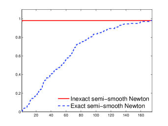
Figure 1: Performance profile comparing Inexact versus Exact semi-smooth Newton method for large-scale sparse AVEs with well conditioned matrices.

Analyzing Figure 1, we see that, as expected, the inexact method is more efficient than the exact one. However, it may be surprising that the difference is so stark. Efficiencies of the methods are $97,5\%$ and $5\%$, respectively, for the inexact and exact versions. The robustness is $98\%$ for both ones. The methods failed to solve the same four problems. Nevertheless, it is interesting to point out that, for this four problems, both methods reached a very close accuracy from the required one to report “Solution found”. In this first set of problems, the exact Newton method was faster in just one problem (21.4s against 35.6s of the inexact method). Curiously, this is the problem for which the condition number of $A$ is the highest value among all considered ones. Considering only the others solved problems, the methods spent in total 201s and 4541s for the inexact and exact versions, respectively. The inexact method solves a typical problem of this set in less than a second while the exact one takes about 20s (in average, the exact method demands 57 times the runtime of the inexact one). The average number of iterations was, respectively, 9.6 and 3.4, showing that, as expected, the exact iteration requests greater computational effort than the inexact one.

Since average condition number of the matrices of the first set problems are relatively small (consequently, in average, the matrices are well conditioned), we investigated the performance of the methods in sets of ill-conditioned matrices. This analysis is pertinent because, as observed, the right hand side of (18) is less than the inverse of condition number. So, for ill-conditioned matrices, the iterative solver for linear equations needs to be much required. It is not reasonable to set a value for the condition number to claim a matrix as “ill-conditioned”. Therefore, in this second phase, we generated two sets of $200$ AVEs. In the first one, the condition numbers of all matrices $A$ are greater than or equal to $10^{2}$ (the average is $4.73\times 10^{2}$) while, in the second one, are greater than or equal $10^{5}$ (the average is $1.72\times 10^{5}$). We emphasize that in these second phase, we keep $n=10000$ and the density of $A$ approximately equal to $0.3\%$. Figure 2 shows a comparison between exact and inexact semi-smooth Newton methods in this two sets of test problems.

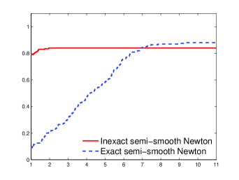
(a)

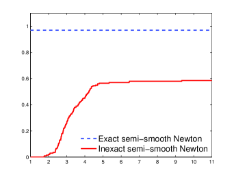
(b)

Figure 2: Performance profile comparing Inexact versus Exact semi-smooth Newton method for large-scale sparse AVEs with “ill-conditioned” matrices: (a) ${\rm cond}(A)\approx 10^{2}$ and (b) ${\rm cond}(A)\approx 10^{5}$.

In the first set of the second phase, analyzing Figure 2(a), we see that the inexact Newton method is more efficient than the exact one (efficiencies are 79% and 9%, respectively), while robustness rates are 84% and 88%, respectively. The robustness difference corresponds to 8 problems that were solved by exact method and failed to be solved by the inexact one. Reciprocally, there is no problem. In others 24 problems, both methods failed. However, in all cases of failure, regardless of the method, the achieved accuracy was close to the desired one (typically, order of $10^{-8}$). This allows us to conclude that both methods were equivalently robust. In terms of processing time, comparing with the set of problems of the first phase, the exact Newton method showed a considerable improvement. Note by Figure 2(a) that the performance functions intersect each other approximately at 7 in the domain, while in Figure 1 the intersection takes place approximately at 160. Consequently, the difference between the two methods is much smaller in the case that the condition number of $A$ is order of $10^{2}$ than in the case where it is order of $10^{1}$.

Consider now the second set of problems where the condition numbers of $A$ are of order of $10^{5}$. Both methods were not able to solve with accuracy $10^{-8}$ an AVE that belongs to this set of ill-conditioned problems. So, in this specific case, we used the accuracy equal to $10^{-5}$. For the inexact method, the average value of $\theta$ is $2.85\times 10^{-6}$. Figure 2(b) shows the performance of the methods. As we can note, the exact Newton method achieved much higher performance compared with the inexact one. The exact method was the faster one in all problems that were solved by both methods. The robustness is $59\%$ and $97\%$ for the inexact and exact method, respectively. The high efficiency of the exact Newton method is connected with the ability of this method to solve a problem with a moderate accuracy ($10^{-5}$) in a few iterations. The exact method did not need more than three iterations in order to solve a problem of this set: 166 problems were solved with 2 iterations, while 28 with 3 iterations. On the other hand, since $\theta$ is oder of $10^{-6}$, the iterative linear equations solver is much required in an early iteration of the inexact method, generating additional runtime. The poor robustness of the inexact method can be related with the lack of robustness of the lsqr routine to deal with ill-conditioned matrices. It is appropriate to mention that no preconditioner was used in lsqr.

Table 1 summarizes the results of the numerical experiments of the current section. The column “${\rm cond}(A)$” informs the (average) order of the condition number of the matrices $A$, while column “$tol$” reports the considered accuracy to solve an AVE.

		Inexact Newton method		Exact Newton method
${\rm cond}(A)$	$tol$	Efficiency ($\%$)	Robustness ($\%$)	Efficiency ($\%$)	Robustness ($\%$)
$10^{1}$	$10^{-8}$	97.5	98.0	5.0	98.0
$10^{2}$	$10^{-8}$	79.0	84.0	9.0	88.0
$10^{5}$	$10^{-5}$	0.0	59.0	97.0	97.0

Table 1: Efficiency and robustness rates of the Inexact and Exact Newton methods for three sets of large-scale sparse AVEs varying the condition number of the matrices.

The numerical experiments of this section allow us to conclude that the inexact Newton method is much more efficient than the exact one when $A$ is a large-scale sparse matrix with a “moderate” condition number. For matrices with higher condition numbers (order of $10^{5}$), both methods failed to solve the AVE problem with accuracy $10^{-8}$. Considering a greater tolerance ($10^{-5}$), the exact method was the most efficient and robust. This indicates that, at least in our implementation, the inexact Newton method is more sensitive to the increase of the condition number than the exact one.

3.2 Influence of Density

The iterative linear equations solvers are suitable for large and sparse matrices, particularly for the routine lsqr. Therefore, in this section, we investigated the influence of the density of matrix $A$ on the performance of the exact and inexact semi-smooth Newton methods. In this third phase, we decided to deal only with relatively “well-conditioned” matrices because, according to the experiments of the previous section, both methods presented greater robustness on this class of problems. Theoretically, it is expected that the huge efficiency difference presented in Figure 1 be reduced.

We generated four sets of $200$ AVEs varying the density of matrix $A$. The density of the matrices in each set is approximately equal to: (a) $10\%$, (b) $40\%$, (c) $80\%$ and (d) $100\%$. The Matlab routine sprand is efficient to generate sparse matrices. When the input density is high, sprand requires much processing time. In order to alleviate this cost, we decided to decrease the dimension of the matrices. In each set of AVEs we adopted $n$ equal to 3000 for the first two sets and 1500 for the other two. The average condition number of the matrices in each set is approximately equal to 11, 35, 17 and 18, respectively. Figure 3 shows the performance profiles, while Table 2 shows the efficiency and robustness rates of the Inexact and Exact Newton methods in this four sets of test problems.

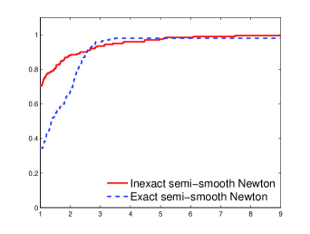
(a)

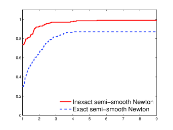
(b)

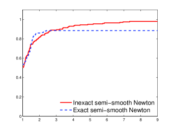
(c)

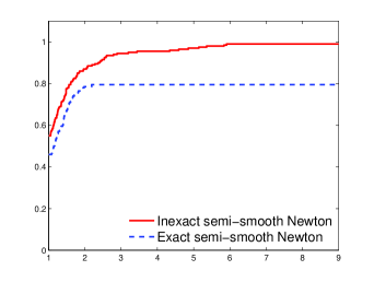
(d)

Figure 3: Performance profile comparing Inexact versus Exact semi-smooth Newton method for dense AVEs with well-conditioned matrices. Density of $A$ is approximately equal to: (a) $10\%$, (b) $40\%$, (c) $80\%$ and (d) $100\%$.

		Inexact Newton method		Exact Newton method
$n$	density ($\%$)	Efficiency ($\%$)	Robustness ($\%$)	Efficiency ($\%$)	Robustness ($\%$)
3000	10	70.5	99.5	34.5	98.0
3000	40	73.5	99.0	30.0	87.0
1500	80	50.5	99.5	53.5	88.5
1500	100	55.0	99.0	46.0	79.5

Table 2: Efficiency and robustness rates of the Inexact and Exact Newton methods for four sets of AVEs varying the density of the matrices.

Analyzing Figure 3 and Table 2, we see that, as expected, the difference between the methods was decreased compared to the case where problems are sparse, see Figure 1. For a moderate density ($10\%$ and $40\%$), the inexact Newton method is more efficient than the exact one (efficiency rate is 70.5$\%$ and 73.5$\%$ against 34.5$\%$ and 30.0$\%$, respectively). Considering full matrices (density $80\%$ and $100\%$) both methods showed equivalent efficiency rates: 50.5$\%$ and 55.0$\%$ for the inexact method against 53.5$\%$ and 46.0$\%$ for the exact one, respectively. Independently of density, the robustness rate of the inexact Newton method is greater than or equal to 99.0$\%$. On the other hand, as we can see in Table 2, the robustness rate of the exact method decreases according to the increase of the density. This phenomenon is clearly connected with the fact that the greater the density, the more operations are required by the direct method to to solve a linear equation. Consequently, the exact Newton method is most affected by the accumulation of floating-point errors resulting in lower robustness. Obviously, the number of operations to solve a linear equation also depends on the dimension $n$. So, considering the exact Newton method, the robustness rate of 87.0$\%$, in the set of problems where $n=3000$ and the density is approximately $40\%$, is consistent with robustness rate of 88.5$\%$ where the dimension and density are $1500$ and approximately $80\%$, respectively.

The numerical experiments of this section allow us to conclude that, at least in problems where $A$ is a “well-conditioned” matrix, the inexact Newton method proved to be competitive (in terms of efficiency) with the exact method even if $A$ is a full matrix. Considering robustness, while the inexact Newton method did not lose performance, the exact method was found to be sensitive with density increase.

4 Final Remarks

In this work we dealt with the global $Q$-linear convergence of the inexact semi-smooth Newton method for solving AVE in (1). In particular, a bound for the relative error tolerance to solve subproblem arises very clearly in the presented results. The inexact analysis support the efficient computational implementations of the exact schemes. Our implementation shows the advantage over the exact method in many considered cases, for instance, sparse and large scale problems. We hope that this study serves as a basis for future research on other more efficient variants for solving AVE. We intend to study the semi-smooth Newton method from the point of view of actual implementations and provide comparisons with alternative approaches. Additional numerical tests indicate that our sufficient condition for convergence can be relaxed, which also deserver to be investigate.

References

- [1] L. Caccetta, B. Qu, and G. Zhou. A globally and quadratically convergent method for absolute value equations. Comput. Optim. Appl., 48(1):45–58, 2011.
- [2] F. H. Clarke. Optimization and nonsmooth analysis, volume 5 of Classics in Applied Mathematics. Society for Industrial and Applied Mathematics (SIAM), Philadelphia, PA, second edition, 1990.
- [3] T. A. Davis. Direct methods for sparse linear systems, volume 2. Siam, 2006.
- [4] R. S. Dembo, S. C. Eisenstat, and T. Steihaug. Inexact Newton methods. SIAM J. Numer. Anal., 19(2):400–408, 1982.
- [5] E. D. Dolan and J. J. Moré. Benchmarking optimization software with performance profiles. Mathematical programming, 91(2):201–213, 2002.
- [6] R. A. Horn and C. R. Johnson. Matrix analysis. Cambridge University Press, Cambridge, 1990. Corrected reprint of the 1985 original.
- [7] J. Iqbal, A. Iqbal, and M. Arif. Levenberg–Marquardt method for solving systems of absolute value equations. J. Comput. Appl. Math., 282:134–138, 2015.
- [8] O. L. Mangasarian. Absolute value programming. Comput. Optim. Appl., 36(1):43–53, 2007.
- [9] O. L. Mangasarian. A generalized Newton method for absolute value equations. Optim. Lett., 3(1):101–108, 2009.
- [10] O. L. Mangasarian. Absolute value equation solution via dual complementarity. Optim. Lett., 7(4):625–630, 2013.
- [11] O. L. Mangasarian. Absolute value equation solution via linear programming. J. Optim. Theory Appl., 161(3):870–876, 2014.
- [12] O. L. Mangasarian. Linear complementarity as absolute value equation solution. Optim. Lett., 8(4):1529–1534, 2014.
- [13] O. L. Mangasarian. Unsupervised classification via convex absolute value inequalities. Optimization, 64(1):81–86, 2015.
- [14] O. L. Mangasarian and R. R. Meyer. Absolute value equations. Linear Algebra Appl., 419(2-3):359–367, 2006.
- [15] J. M. Ortega. Numerical analysis, volume 3 of Classics in Applied Mathematics. Society for Industrial and Applied Mathematics (SIAM), Philadelphia, PA, second edition, 1990. A second course.
- [16] C. C. Paige and M. A. Saunders. Lsqr: An algorithm for sparse linear equations and sparse least squares. ACM Transactions on Mathematical Software (TOMS), 8(1):43–71, 1982.
- [17] O. Prokopyev. On equivalent reformulations for absolute value equations. Comput. Optim. Appl., 44(3):363–372, 2009.
- [18] L. Q. Qi and J. Sun. A nonsmooth version of Newton’s method. Math. Programming, 58(3, Ser. A):353–367, 1993.
- [19] J. Rohn. A theorem of the alternatives for the equation . Linear Multilinear Algebra, 52(6):421–426, 2004.
- [20] J. Rohn, V. Hooshyarbakhsh, and R. Farhadsefat. An iterative method for solving absolute value equations and sufficient conditions for unique solvability. Optim. Lett., 8(1):35–44, 2014.
- [21] D. K. Salkuyeh. The Picard-HSS iteration method for absolute value equations. Optim. Lett., 8(8):2191–2202, 2014.
- [22] C. Zhang and Q. J. Wei. Global and finite convergence of a generalized Newton method for absolute value equations. J. Optim. Theory Appl., 143(2):391–403, 2009.