Hierarchical fragmentation and collapse signatures in a high-mass starless region.

Abstract

Aims. Understanding the fragmentation and collapse properties of the dense gas during the onset of high-mass star formation.

Methods. We observed the massive ($\sim$800 M_⊙) starless gas clump IRDC 18310-4 with the Plateau de Bure Interferometer (PdBI) at sub-arcsecond resolution in the 1.07 mm continuum and N₂H⁺(3–2) line emission.

Results. Zooming from a single-dish low-resolution map to previous 3 mm PdBI data, and now the new 1.07 mm continuum observations, the sub-structures hierarchically fragment on the increasingly smaller spatial scales. While the fragment separations may still be roughly consistent with pure thermal Jeans fragmentation, the derived core masses are almost two orders of magnitude larger than the typical Jeans mass at the given densities and temperatures. However, the data can be reconciled with models using non-homogeneous initial density structures, turbulence and/or magnetic fields. While most sub-cores remain (far-)infrared dark even at 70 $\mu$m, we identify weak 70 $\mu$m emission toward one core with a comparably low luminosity of $\sim$16 L_⊙, re-enforcing the general youth of the region. The spectral line data always exhibit multiple spectral components toward each core with comparably small line widths for the individual components (in the 0.3 to 1.0 km s^-1 regime). Based on single-dish C¹⁸O(2–1) data we estimate a low virial-to-gas-mass ratio $\leq 0.25$. We discuss that the likely origin of these spectral properties may be the global collapse of the original gas clump that results in multiple spectral components along each line of sight. Even within this dynamic picture the individual collapsing gas cores appear to have very low levels of internal turbulence.

1 Introduction

Independent of the various formation scenarios for high-mass stars that are discussed extensively in the literature (e.g., Zinnecker & Yorke 2007; Beuther et al. 2007; Tan et al. 2014), the initial conditions required to allow high-mass star formation at all are still poorly characterized. The initial debate even ranged around the question whether high-mass starless gas clumps should exist at all, or whether the collapse of massive gas clumps starts immediately without any clear starless phase in the high-mass regime (e.g., Motte et al. 2007). Recent studies indicate that the time span during which massive gas clumps exist without embedded star formation is relatively short (on the order of 50000 yrs), but nevertheless, high-mass starless gas clumps do exist (e.g., Russeil et al. 2010; Tackenberg et al. 2012; Csengeri et al. 2014). Current questions in that field are: are high-mass gas clumps dominated by a single fragment or do we witness strong fragmentation during earliest evolutionary stages (e.g., Bontemps et al. 2010; Zhang et al. 2015)? What are the kinematic properties of the gas (Dobbs et al., 2014)? Are the clumps sub- or super-virial (Tan et al., 2014)? Do we see streaming motions indicative of turbulent flows (e.g., Bergin et al. 2004; Vázquez-Semadeni et al. 2006; Heitsch et al. 2008; Banerjee et al. 2009; Motte et al. 2014; Dobbs et al. 2014)?

To address such questions, one needs to investigate the earliest evolutionary stages prior to the existence of embedded heating and outflow sources that could quickly destroy any signatures of the early kinematic and fragmentation properties. Furthermore, high-spatial resolution is mandatory to resolve the important sub-structures at typical distances of several kpc. To get a taste of the important scales, we can estimate typical Jeans lengths for high-mass star-forming regions: for example, average densities $\rho$ of high-mass star-forming gas clumps on $\sim 0.5$ pc scale in the $10^{5}$ cm^-3 density regime at low temperatures of 15 K result in typical Jeans fragmentation scales of $\sim$10000 AU. Going to smaller spatial scales ($\leq 0.1$ pc), the embedded cores have higher densities in the $10^{6}$ cm^-3 regime that result in much smaller Jeans fragmentation scales on the order of 4000 AU (e.g., Beuther et al. 2013b).

Our target region IRDC 18310-4 is a 70 $\mu$m dark high-mass starless region at 4.9 kpc distance that was previously observed with the PdBI in the CD configuration in the 3 mm continuum and the N₂H⁺(1–0) emission with a spatial resolution of $4.3^{\prime\prime}\times 3.0^{\prime\prime}$ (Beuther et al., 2013b). We identified fragmentation and core formation of the still starless gas clump, and approximate separations between the separate cores are on the order of 25000 AU. Fragmentation of these cores could not be resolved by the previous observations. The simultaneously observed N₂H⁺(1–0) data exhibit at least two velocity components. Such multi-velocity-components are the expected signatures of collapsing and fragmenting gas-clumps (Smith et al., 2013).

In a hierarchically structured star-forming region, the cores are the supposed entities where further fragmentation should take place and which likely contain bound multiple systems. Studying this region now at 1.07 mm in the dust continuum and N₂H${}^{+}(3-2)$ at sub-arcsecond resolution reveals the hierarchical fragmentation and kinematic properties of the densest cores at the onset of high-mass star formation.

2 Observations

2.1 Plateau de Bure Interferometer

The target region IRDC 18310-4 was observed with the Plateau de Bure Interferometer at 1.07 mm wavelength in the B and C configuration in 4 tracks in March and November 2013. The projected baselines extended to approximately 420 m. The 1 mm receivers were tuned to 279.512 GHz in the lower sideband. At the given wavelength, the FWHM of the primary beam is approximately $18^{\prime\prime}$, and we used a small 2-field mosaic to cover our region of interest. Phase and amplitude calibration was conducted with regular observations of the quasars 2013+370 and 1749+096. The absolute flux level was calibrated with MWC349 and bandpass calibration was done with 3C84. We estimate the final flux accuracy to be correct to within $\sim 15\%$. The phase reference center is RA (J2000.0) 18:33:39.532 and Dec (J2000.0) -08:21:09.60, and the velocity of rest $v_{\rm{lsr}}$ is $\sim$86.5 km s^-1. While the channel spacing of the correlator was 0.084 km s^-1, to increase the signal-to-noise ratio we imaged the data with 0.2 km s^-1 spectral resolution. For the continuum and line data we used different weighting systems between natural and uniform weighting to improve the signal-to-noise ratio in particular for the line data. The resulting synthesized beam for the continuum and N₂H⁺(3–2) data were $0.6^{\prime\prime}\times 0.49^{\prime\prime}$ (with a position angle of $11^{o}$) and $1.13^{\prime\prime}\times 0.5^{\prime\prime}$ (with a position angle of $13^{o}$), respectively. The corresponding $1\sigma$ rms for the two data sets is $\sim$0.6 mJy beam^-1 and $\sim$15 mJy beam^-1 measured in a line-free channel of 0.2 km s^-1 for the line data.

2.2 Herschel PACS

The Herschel data were already presented in Beuther et al. (2013a). However, they were fully re-calibrated for this analysis with particular emphasis to applying the most recent pointing and astrometry solutions. The region containing IRDC 18310-4 was observed with the Herschel spacecraft (Pilbratt et al., 2010) within the Key Project EPoS (Ragan et al., 2012). The related observations utilizing the bolometer cameras of PACS (Poglitsch et al., 2010) took place on April 19, 2011 (operational day 705) and were contained in the observational IDs 1342219060–63. The PACS prime mode was employed with a nominal scanning velocity of 20^′′ second^-1. Data were taken in all three PACS filters (70, 100, and 160 $\mu$m) and resulted in maps with roughly 10 arcmin field-of-view. We re-reduced the existing Herschel archive data, starting from the Level1 data. These we retrieved from the previous bulk processing with the HIPE 12.1 software version, currently contained in the HSA. We included the newly developed data reduction step calcAttitude: a correction of the frames pointing product based on the Herschel gyroscope house-keeping (Sánchez-Portal et al., 2014). This often improves the absolute pointing accuracy and mitigates the pointing jitter effect on individual frames. We used these corrected frames and performed the individual detector pixel distortion correction, the de-striping, the removal of 1/f noise, and the final map projection using Scanamorphos (Roussel, 2013), version 24, employing the “galactic” option. The resulting full width half maximum (FWHM) of the point spread function (PSF) at 70, 100, and 160 $\mu$m are $5.6^{\prime\prime}$, $6.8^{\prime\prime}$ and $11.3^{\prime\prime}$, respectively.

3 Results

3.1 Millimeter continuum emission

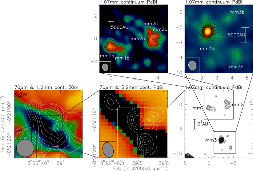
Figure 1: Compilation of the continuum images in IRDC 18310-4. The bottom-left and middle panels show in color the Herschel 70 $\mu$m image with a stretch going dark for low values (Beuther et al. 2013b, linear and log stretch for clarity, respectively). The white contours in the left panel show the 1.2 mm MAMBO continuum observations starting from 4$\sigma$ and continuing in 1$\sigma$ steps with a $1\sigma$ value of 13 mJy beam^-1. The contours in the bottom-middle panels presents the 3 mm continuum data from Beuther et al. (2013b) starting from 3$\sigma$ and continuing in 2$\sigma$ steps with a $1\sigma$ value of 0.08 mJy beam^-1. The bottom-right panel then shows the new 1.07 mm continuum observations starting from 3$\sigma$ and continuing in 1$\sigma$ steps with a $1\sigma$ value of 0.6 mJy beam^-1. The two top panels show zooms of the 1.07 continuum data with the same contour levels but a different color stretch to highlight the sub-structures. Each panel presents scale-bars and the corresponding synthesized beams. The 70 $\mu$m PSF is $5.6^{\prime\prime}$.

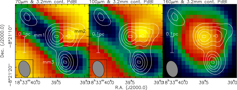
Figure 2: Re-calibrated Herschel PACS images at 70, 100 and 160 $\mu$m (from left to right). The scaling in the three panels is from -3.8 to 4.0, from 5.0 to 17.6, and from 33 to 45 mJy pixel^-1, respectively. The 3.2 mm continuum contours are from 3$\sigma$ and continuing in 2$\sigma$ steps with a $1\sigma$ value of 0.08 mJy beam^-1. A scale-bar and the 3.2 mm synthesized beam are shown in each panel, and the three main sources are labeled in the bottom-left panel. The 70, 100, and 160 $\mu$m PSFs are $5.6^{\prime\prime}$, $6.8^{\prime\prime}$ and $11.3^{\prime\prime}$, respectively.

Figure 1 presents a compilation of the 70 $\mu$m and 1.2 mm single-dish data (Ragan et al., 2012; Beuther et al., 2002), the previous 3.2 mm PdBI continuum observations (Beuther et al., 2013b) as well as our new 1.07 mm PdBI continuum maps. The three datasets cover a broad range of resolution elements from $11^{\prime\prime}$ in the MAMBO 1.2 mm data, to $4.3^{\prime\prime}\times 3.0^{\prime\prime}$ in the 3.2 mm PdBI data, to $0.6^{\prime\prime}\times 0.49^{\prime\prime}$ in our new 1.07 mm observations. At the given distance of 4.9 kpc, this corresponds to linear resolution elements of $\sim 54000$ AU, $\sim 18000$ AU and $\sim 2700$ AU, respectively. With the different resolution elements, we can clearly identify hierarchical fragmentation on the different scales of our observations: the large-scale single-dish gas clump with a total mass of $\sim 800$ M_⊙ fragments into 4 cores with masses between 18 and 36 M_⊙ (Beuther et al., 2013b), and these cores again fragment into smaller sub-structures in our new 1.07 mm continuum data. For our following analysis, we only consider 1.07 mm sources that are detected at a $>4\sigma$ level. We can estimate the masses and column densities of these smallest-scale structures with similar assumptions as taken in Beuther et al. (2013b), namely optically thin dust emission at a low temperature of 15 K (see also sect. 3.2), with a gas-to-dust ratio of 150 (Draine, 2011) and dust properties discussed in Ossenkopf & Henning (1994) for thin ice mantles at densities of $10^{5}$ cm⁻³ ($\kappa_{1.07{\rm mm}}\sim 0.95$ cm² g^-1). Main uncertainties for the mass and column density estimates are the applied dust model and the assumed temperature. Based on this, we estimate an accuracy within a factor 2 for these parameters. This way, we estimate the masses of the smallest-scale substructures to values between 2.2 and 19.3 M_⊙ (Table 1). The difference of the sum of the core masses compared to the large-scale single-dish mass of $\sim 800$ M_⊙ is mainly caused by the spatial filtering of the interferometer that traces only the densest inner cores and not the envelope anymore. The peak column densities are very high in the regime of $10^{24}$ cm^-2, corresponding to visual extinctions of $\sim 1000$ mag.

Table 1: Fluxes, masses and column densities

	$S_{\rm{int}}$	$S_{\rm{peak}}$	$M$	$N_{\rm{H_{2}}}$
	(mJy)	$\left(\frac{\rm{mJy}}{\rm{beam}}\right)$	(M⊙)	($10^{24}$cm-2)
mm1	12.01		9.71
mm1a	8.2	4.1	6.6	1.1
mm1b	3.8	2.9	3.1	0.8
mm2	17.02		13.72
mm2a	4.5	3.8	3.6	1.0
mm2b	4.7	3.8	3.8	1.0
mm2c	3.3	3.3	2.7	0.9
mm3a	24.0	14.0	19.3	3.8
mm3b	2.7	2.7	2.2	0.7
mm3c	3.5	3.5	2.8	0.9

Uncertainties for $S_{\rm{int}}$ and $S_{\rm{peak}}$ are $\approx$15% (§2). Uncertainties for$M$ and $N_{\rm{H_{2}}}$ are approximately a factor 2 (§3.1).
¹ Integrated over mm1 & mm1a
² Integrated over mm2a, mm2b & mm2c

Table 2: Projected nearest neighbor separations

	(”)	(AU)
3mm data
mm1–mm2	2.9	14200
mm1–mm3	7.1	34900
1mm data
mm1a–mm1b	0.9	4400
mm2a–mm2b	0.5	2600
mm2a–mm2c	0.7	3500
mm2b–mm2c	1.1	5500
mm3a–mm3b	1.5	7600
mm3a–mm3c	2.5	12000
mm3b–mm3c	2.4	11900

Uncertainties are $\approx$0.1^′′ or $\approx$490 AU.

In addition to the masses and column densities, the data allow us to estimate the fragmentation properties of the sub-sources, and we find projected separations between the newly identified structures between 2600 and 12000 AU (Table 2). Since the absolute peak positions can be determined to high accuracy ($\frac{\phi}{S/N}$ with the resolution $\phi$ and the signal-to-noise ratio $S/N$, e.g., Reid et al. 1988), and the intereferometric positional accuracy depends mainly on the position of the used quasar and its gain calibration solution (within $0.1^{\prime\prime}$), the projected separation is estimated to be accurate within $0.1^{\prime\prime}$ or 490 AU. A fragmentation discussion is presented in section 4.1.

3.2 Far-infrared continuum emission

Figure 2 presents a comparison of the Herschel PACS 70, 100 and 160 $\mu$m data with the 3.2 mm continuum data from the PdBI. At 70 $\mu$m, large parts of the central region containing the millimeter cores still appear as a dark extinction silhouette in front of the extended 70 $\mu$m emission of the hosting molecular cloud (Figures 1 & 2). Although the extinction contrast decreases at 100 $\mu$m, we still perceive the central parts as an infrared dark cloud (IRDC). At 160 $\mu$m, the extended emission in the surroundings is not so dominating anymore, and emission structures emerge from the inside of the IRDC.

At the north-western border of the IRDC silhouette, we notice a faint emission point source at 70 $\mu$m which also persists at 100 $\mu$m. In the previous data reduction products we used in Ragan et al. (2012) and Beuther et al. (2013a), this source was not that apparent. We attribute the differences to the use of the newest Scanamorphos algorithms and the inclusion of the gyro-correction information (Sect. 2.2) in the current data reduction. In order to determine accurate positions, we referenced the PACS maps with the Spitzer/MIPSGAL (Carey et al., 2009) 24 $\mu$m data. We did not use individual MIPSGAL maps for reference, but relied on the recently released MIPSGAL 24 $\mu$m point source catalogue (Gutermuth & Heyer, 2015). Corresponding positions in the PACS maps were determined by employing PSF photometry using IDL/Starfinder (Diolaiti et al., 2000). The necessary adjustments were shifts on the order of 1.1–1.6^′′. For the previous Herschel data products (with uncorrected pointing) we had to use a shift of almost $4^{\prime\prime}$ (Beuther et al., 2013a). This supports predictions that the absolute pointing error of Herschel data can be brought down to a level of $\sim$0$\aas@@fstack{\prime\prime}$9 1$\sigma$ if all the recent corrections for the pointing product are applied (Sánchez-Portal et al., 2014). This 70 $\mu$m point source is thus located very close to mm2. Interestingly, the compact emission seen at 160 $\mu$m is shifted towards the center of the IRDC and basically coincides with the mm1 location (Fig. 2). The uncertainties of the peak positions are on the order of 1^′′ for 70 and 100 $\mu$m, due to the position bootstrapping involved. For the 160 $\mu$m astrometry, the uncertainty might even be up to $2^{\prime\prime}$, since at this wavelength it is hard to find real point sources, and due to extended emission and large beam sizes, the effective peak position may experience subtle displacements (cf. the comparison of MIPS-70 and PACS-70 $\mu$m peaks for the EPoS source UYSO1 reported in Linz et al. 2010). Still, the formal distance between the 70 $\mu$m point source and the 160 $\mu$m compact emission peak is more than 4^′′. Although this is less than the beam of the 70 $\mu$m image, as mentioned in §3.1, source peak positions can be determined to much higher accuracy than the nominal spatial resolution $\phi$ (down to $\frac{\phi}{S/N}$). Hence, we think that there is a real shift in peak positions when going to longer wavelengths. This may be explainable by the combined action of two effects. First, the 160 $\mu$m data trace colder dust expected in the deeper interior of the IRDC, compared to the 70 $\mu$m wavelength range. Second, the 160 $\mu$m beam is around 11$\aas@@fstack{\prime\prime}$3. It thus convolves emission from larger areas, and therefore may comprise emission from mm1 (dominating) and mm2 (minor contribution), while the finer 70 $\mu$m beam of 5$\aas@@fstack{\prime\prime}$6 can still distinguish between mm2 (associated with 70 $\mu$m emission at its north-west side) and mm1 (without noticeable 70 $\mu$m emission).

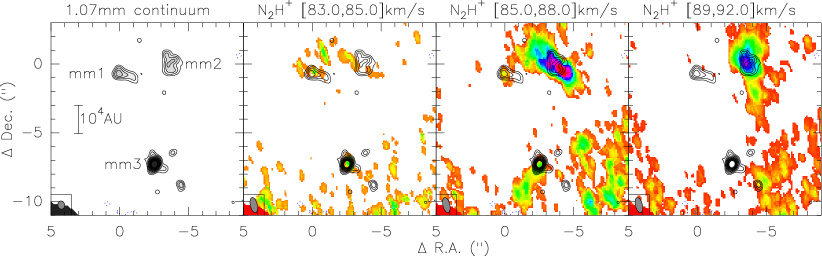
Figure 3: N₂H${}^{+}(3-2)$ and 1.07 mm continuum data. The left panel and the contours in the three other panels always show the 1.07 mm continuum data starting from 3$\sigma$ and continuing in 1$\sigma$ steps with a $1\sigma$ value of 0.6 mJy beam^-1. The color-scale in the 2nd, 3rd and 4th panels present the N₂H${}^{+}(3-2)$ integrated emission over the velocity regimes marked above each panel. The scaling ranges in panel 2 to 4 are [0,0.15], [0,0.25] and [0,0.4] Jy km s^-1, respectively. The synthesized beam of the continuum and line data is shown each time in the bottom-left. A scale-bar can be found in the left panel.

Table 3: Far-infrared fluxes of mm2

$\lambda$	$S$
($\mu$m)	(mJy)
70	90
100	357
1601	$\leq$339
32302	0.9

Flux uncertainties at 70 and 100 $\mu$m are $\sim$10%.
¹ Upper limit from the residual flux toward mm2 after subtracting the point source centered on mm1.
² From Beuther et al. (2013a) with an accuracy of $\sim$15%.

Hence, the PACS data show tentatively that at least object mm2 may not be totally starless anymore, but that star formation processes might have begun at its north-western border. Whether the 70 $\mu$m point source is already a recently formed protostar, or just a temperature enhancement created by various processes triggered from within mm2, is not easy to answer with the presently available data. At 160 $\mu$m, we eventually see the cold dust emission from the bulk of the core material in the mm1/2 region.

The Herschel data can also be used to get a rough estimate of the luminosity of the mm2 core. In the 70 and 100 $\mu$m band, we were able to derive the far-infrared fluxes toward mm2 from fitting the point-spread-function (PSF) to the compact emission source visible in Fig. 2. The uncertainties for the 70 and 100 $\mu$m flux measurements are $\approx$10%, including $\sim$5% calibration uncertainty and another $\sim$5% from the PSF photometry. At 160 $\mu$m, this is more difficult because the emission peaks at mm1. Therefore, in this band we can only derive an upper limit for mm2 by fitting a point source to mm1, and afterwards deriving the mm2 upper limit from the residual image. The 3 mm flux density was taken from Beuther et al. (2013a). Fitting a spectral energy distribution to these four data points assuming a modified blackbody function accounting for the wavelength-dependent emissivity of the dust, we get an estimate of the luminosity $L$ and cold dust temperature $T_{\rm{dust}}$. For mm2, this results in $L\sim 16_{-8}^{+14}$ L_⊙ and $T_{\rm{dust}}\sim 15_{-0.5}^{+2.0}$ K. The error budget in $L$ and $T_{\rm{dust}}$ includes the uncertainties of the flux calibration as well as the selected dust model. While the dust temperature reflects the overall cold nature of this region, the comparably low internal luminosity of mm2 around 16 L_⊙ shows that this region with a large mass reservoir of $\sim$800 M_⊙ (section 3.1) still has formed no high-mass star yet. It should also be noted that the low luminosity cannot be explained well with accretion processes on compact protostars because even then the accretion luminosity is expected to be higher (e.g., Krumholz et al. 2007). Hence, the observed luminosity may likely stem from accretion processes on larger surfaces, re-enforcing the early evolutionary stage at the onset of star formation with active collapse processes.

Looking closer at mm3, there is no emission at 70 and 100 $\mu$m, and the 160 $\mu$m image exhibits only a very weak extension from mm1 in the direction of mm3. This is in stark contrast to the 3.2  and 1.07 mm data which exhibit almost the same fluxes for mm1 and mm3. This difference is most likely due to even lower temperatures within the mm3 region compared to mm1.

3.3 Spectral line emission

Figure 3 presents several N₂H⁺(3–2) emission maps integrated each time over different velocity regimes. The velocity regimes are selected based on the integrated N₂H⁺(3–2) spectrum presented in the bottom panel of Fig. 4. We divide the integrations into a low-velocity part between 83 and 85 km s^-1, an intermediate-velocity regime between 85 and 88 km s^-1 and a high-velocity part from 89 to 92 km s^-1. The immediate result of that is that the different velocities trace different parts of the dense gas. While the low-velocity component is mainly associated with the sub-sources mm1 and mm3, the intermediate-velocity component emits toward all three mm cores, and finally the high-velocity component emits only toward mm2. Although the N₂H⁺(3–2) line has hyperfine-structure as well, the satellite lines are comparably weak, and the velocity structure is mainly caused by real structure imposed on the main hyperfine component. Nevertheless, we also fit the spectra taking into account the full hyperfine structure of the line (see below). Independent of that, these integrated emission images already show that this high-mass starless clump is far from being a kinematically homogeneous and potentially calm structure, but in contrast to that, we see a kinematically complex region that may be at the verge of collapse (see also Ragan et al. 2015).

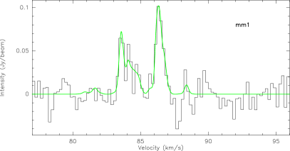
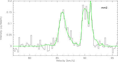
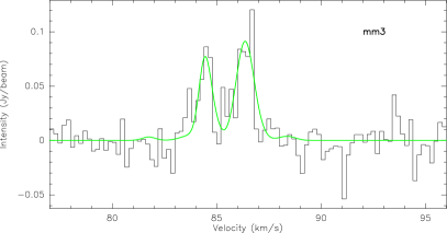
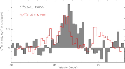
Figure 4: N₂H${}^{+}(3-2)$ spectra toward the three main peaks mm1, mm2 and mm3 with the multiple component hyperfine-structure fits shown in green. The fit parameters are presented in Table 4. The bottom spectrum shows a comparison between a single-dish C¹⁸O(2–1) spectrum extracted toward the main peak in grey-scale, whereas the red spectrum is an average of the three above N₂H${}^{+}(3-2)$ spectra (multiplied by 8). The units in the bottom spectra are different for both as marked in the side-label.

To investigate the kinematics in more depth, we extracted the spectra toward the three main mm cores mm1, mm2 and mm3, which are shown in Figure 4. Again, the multiple velocity components are apparent. To quantify the peak velocities $v_{\rm{peak}}$ and full-width half maximum $\Delta v$, we fitted the full N₂H⁺(3–2) hyperfine structure to these lines with multiple components. Note that, in contrast to the 1–0 transition, for the 3–2 transition of N₂H⁺ the spectrum is much more strongly dominated by the central line component. From the 29 hyperfine structure components more than 60% of the relative intensities are within the central 6 components separated by only $\sim$0.06 km s^-1 whereas the remaining 23 components share the rest of the emission. The resulting fits are shown in Table 4. One should keep in mind that the selection of the number of fitted velocity components is partly ambiguous. For example, for mm2 we fitted in total three components but one could also have fitted the high-velocity feature in mm2 with three components alone and have a fourth component around the intermediate-velocity gas. Therefore, these fits do not claim to be the final answer, but they nevertheless adequately represent the current data. While the multiple components toward individual peaks are interesting in themselves, also the derived line width are important. They range in full-width-half-maximum (FWHM) between 0.3 and 1.3 km s^-1 where the 0.3 km s^-1 have to be considered as an upper limit because with our velocity resolution of 0.2 km s^-1 no narrower lines can be resolved. The broad end of the distribution is most likely also an upper limit, however this time caused by unresolved underlying spectral multiplicity in the lines. With the thermal line width at 15 K of $\sim$0.15 km s^-1, these new data now resolve the spectra into almost thermal lines, just with multiple components.

For comparison, Figure 4 also shows a single-dish C¹⁸O(2–1) spectrum at $11^{\prime\prime}$ resolution (Ragan et al. priv. comm.) as well as the PdBI N₂H⁺(3–2) spectrum integrated over all three mm continuum cores. While the C¹⁸O spectrum easily traces the main intermediate-velocity component, however spectrally not well resolved in the sub-components (a Gaussian two-component fit to the C¹⁸O(2–1) spectrum results in $\Delta v$ values of $\sim$1.7 and $\sim$0.3 km s^-1, a 1-component fit has $\Delta v\sim 2.0$ km s^-1), the high- and low-velocity components are not seen at all in the C¹⁸O(2–1) spectrum. The reason for that is likely at least twofold and lies within the lower spatial resolution of the single-dish data as well as the about two orders of magnitude lower critical density of C¹⁸O(2–1) compared to N₂H⁺(3–2) ($\sim 10^{4}$ versus $\sim 10^{6}$ cm^-3). With the new high-resolution observations of this dense gas tracer, we are able to really dissect the densest portions of this very young high-mass star-forming region (see section 4.2).

Table 4: Hyperfine structure fits toward the mm peaks

	$v_{\rm{peak}}$	$\Delta v$
	(km s-1)	(km s-1)
mm1	83.5	0.3
mm1	84.3	0.3
mm1	86.3	0.3
mm2	85.8	1.3
mm2	89.9	0.7
mm2	91.0	0.3
mm3	84.4	0.6
mm3	86.2	0.9

4 Discussion

We now have the ability to track the hierarchical fragmentation and global collapse of starless gas clumps capturing smaller and smaller scales.

4.1 Fragmentation

Following Beuther et al. (2013b), we can estimate the average densities $\rho$ for the large-scale single-dish data as well as the previous intermediate-scale 3 mm continuum data, corresponding to the bottom-left and bottom-middle panels in Figure 1. The estimated average densities $\rho$ derived from the two datasets are $2.5\times 10^{5}$ cm^-3 and $1.5\times 10^{6}$ cm^-3, respectively. Assuming furthermore average temperatures of 15 K, Beuther et al. (2013b) estimated the Jeans length $\lambda_{\rm Jeans}$ and Jeans mass $M_{\rm Jeans}$ that predict the expected fragment properties of the corresponding smaller scales in the framework of this isothermal gravitational Jeans fragmentation picture. The $\lambda_{\rm Jeans}$ and $M_{\rm Jeans}$ based on the large-scale single-dish data are 10000 AU and 0.37 M_⊙, whereas the corresponding $\lambda_{\rm Jeans}$ and $M_{\rm Jeans}$ derived from the intermediate-scale 3 mm PdBI data are 4000 AU and 0.15 $M_{\odot}$ (Beuther et al., 2013b).

If we now compare the predicted length and mass scales with the corresponding observed values on the different scales, we find correspondences as well as differences. Regarding the Jeans length and the observed projected separations, the predicted Jeans length from the single-dish data of $\sim$10000 AU is slightly smaller than the core separation in the PdBI 3.2 mm data (Table 2), but the values are consistent within a factor of a few. Going to smaller scales, the predicted Jeans length from the 3.2 mm data of $\sim$4000 AU is roughly consistent with the projected separations we find again at the smaller scales of the 1.07 mm continuum data (Table 2). Hence, from a pure length-scale argument, the observations of IRDC 18310-4 would be roughly consistent with classical thermal Jeans fragmentation. However, our observations reveal only projected separations, and the real ones can be roughly up to a factor 2 larger.

Does this picture also hold for the Jeans masses? In fact, it does not because the predicted Jeans masses on the different scales of 0.37 and 0.15 $M_{\odot}$, respectively, are significantly lower than what is found in the 3.2 mm data (masses for mm1 to mm3 between 18 and 36 $M_{\odot}$, Beuther et al. 2013b) as well as in our new 1.07 mm observations (masses between 2.2 and 13.7 M_⊙, Table 1). Hence, while the length scales are roughly consistent between the classical Jeans predictions and the data, the masses deviate by up to two orders of magnitude. We note that these observed masses are even only lower limits because large fractions of the gas are filtered out.

Similar discrepancies were recently reported by Wang et al. (2014) in their fragmentation study of parts of the “Snake” filament. They also found projected separations in their data that correspond reasonably well to the estimated Jeans length, whereas the fragment masses exceeded the Jeans masses by similar margins as in our data. They argued that the typical thermal Jeans mass is calculated with the thermal sound speed depending on the temperature of the gas. However, Wang et al. (2014) evaluate a turbulent Jeans mass using the turbulent velocity dispersion of the gas instead of the velocity dispersion based on the thermal sound speed. Since the Jeans mass depends on the velocity dispersion to the third power, even velocity dispersion increases of a factor of a few allow to shift the turbulent Jeans masses by more than an order of magnitude in their regime of observed masses. Hence, Wang et al. (2014) argue that turbulent Jeans fragmentation may explain the observed properties. A first-order inconsistency could arise in this picture when considering the lengths scales. In the turbulent Jeans scenario, also the turbulent Jeans length has to be adapted according to the turbulent velocity dispersion. Although the velocity dispersion only enters the equation for the Jeans length linearly, nevertheless, it increases the turbulent Jeans length by a factor of a few. And in that picture, the projected separations of their cores would be a factor of a few smaller than the predicted turbulent Jeans length. However, taking into account potential projection effects, this difference may be less severe.

This turbulent Jeans fragmentation picture becomes questionable for IRDC 18310-4 if one considers that toward one of our most massive sub-condensations mm1a with 6.6 M_⊙ the measured line widths only shows upper limits of 0.3 km s^-1. Hence, no significant turbulent contribution to the line-width is observed here.

A different approach to solve the discrepancies between the classical Jeans fragmentation and our data is to investigate the initial conditions, in particular the initial density structure. While the Jeans fragmentation analysis starts with uniform and infinite gas structures (e.g., Stahler & Palla 2005), the derived density structures of the observed gas clumps exhibit much steeper density profiles (e.g., Beuther et al. 2002; Mueller et al. 2002; Hatchell & van der Tak 2003). Girichidis et al. (2011) analyzed the different fragmentation properties during star formation in numerical simulations varying the turbulent velocity fields as well as the density profiles from uniform to Bonnor-Ebert sphere and density power-law profiles $\rho\propto r^{-p}$ with indices $p$ of 1.5 and 2. As expected, the steeper the initial density profile is, the less fragmentation they find and the more massive the final fragment masses are. In the extreme cases, the difference in masses rises by up to a factor $\sim$20. While they do not explicitly give the fragment separations, the fact that they find less fragments, indicates that the fragment separation should also increase.

To summarizes these effects, most likely, the observed fragmentation properties in IRDC 18310-4, as well as other sources in the literature, could be explained by turbulence-suppressed fragmentation of gas clumps with non-uniform density structures. Magnetic fields can be another agent in inhibiting fragmentation (e.g., Commerçon et al. 2011; Pillai et al. 2015).

4.2 Kinematic properties

As outlined in section 3.3, our new high-spatial and high-spectral resolution observations of the dense gas tracer N₂H⁺(3–2) resolve the spectral lines from the several cores into multiple spectral components where the individual components are only slightly above the thermal line width. Although the data are not good enough yet to actually resolve coherent thermally dominated structures like those found for example in B5 (Pineda et al., 2010, 2015), we are reaching a regime for the individual sub-cores within a high-mass star-forming region that is not that far apart from coherence.

However, in addition to the narrow line widths found for individual components, the omnipresence of multiple components toward each core implies additional highly dynamic processes within the overall high-mass star-forming region. The most straightforward interpretation of these multiple velocity components is within the picture of a globally collapsing gas clump where the different velocity components trace separate individual gas parcels that fall toward the gravitational center of the whole gas clump. The spectral line N₂H⁺(1–0) signatures of such a global collapse were simulated by Smith et al. (2013), and they find similar spectra with multiple components along individual line of sights as seen in our IRDC 18310-4 data.

The C¹⁸O(2–1) data allow us also to derive a rough estimate of the virial mass. Following MacLaren et al. (1988) assuming a density profile $\rho\propto 1/r$, a radius of the clump of 0.25 pc (Fig. 1) as well as the 1-component fit $\Delta v\sim 2.0$ km s^-1 to the C¹⁸O(2–1) spectrum, the approximate virial mass is $\sim$190 M_⊙, about a factor 4 lower than the gas mass of 800 M_⊙ derived from the dust continuum data (Beuther et al., 2013b).

In the framework of a globally collapsing gas clump, one can use the observed spectral velocity differences also for a simple collapse time estimate. Assuming that the difference between the velocity peaks is due to cores sitting at different points in a globally collapsing region, we get converging velocity differences along the lines of sight of 2.8 km s^-1 in mm1, 5.2 km s^-1 in mm2, and 1.8 km ^-1s in mm3. Ignoring for this estimate the plane of the sky velocity component that we do not know, these velocity gradients would bring together fragments 10000 AU apart in only $\sim 1\times 10^{4}$ to $\sim 2.6\times 10^{4}$ yrs. The collapse of the clump may also cause the fragments to merge or increase in density, which could help explain the high fragment masses in the previous section. For example, Smith et al. (2009) found, using synthetic interferometry observations of simulated gas clumps, that the number of fragments decreased and their mean column density increased as the clumps collapsed. This could efficiently increase the mass of the fragments.

Combining the multiple components with the individual narrow line widths as well as the low virial mass, we interprete the kinematic data in this region as most likely caused by a dynamical collapse of a large-scale gas clump that caused multiple velocity components along the line of sight, and where at the same time the individual infalling gas structures have very low levels of internal turbulence.

5 Conclusions

Resolving the mm continuum and N₂H⁺(3–2) emission at sub-arcsecond resolution (linear scales down to $\sim$2500 AU) toward the pristine high-mass starless gas clump IRDC 18310-4, we reveal the fragmentation and kinematic properties of the dense gas at the onset of massive star formation. Zooming through different size scales from single-dish data to intermediate- and high-angular resolution PdBI observations, the resolved entities always fragment hierarchically into smaller sub-structures at the higher spatial resolution. While the fragment separations are still in approximate agreement with thermal Jeans fragmentation, the observed core masses are orders of magnitude larger than estimated Jeans masses at the given densities and temperatures. Hence, additional processes have to be in place. However, taking into account non-uniform density structures as well as initial turbulent gas properties, observed core masses and projected separations are consistent with cloud formation models.

While most sub-cores are (far-)infrared dark even at 70 $\mu$m, the re-reduced Herschel data reveal weak 70 $\mu$m emission toward core mm2 with a comparably low luminosity of only $\sim$16 L_⊙. Since such a low luminosity can be caused neither by an internal high-mass star nor by strong accretion onto a typical embedded protostar, this re-enforces the youth and early evolutionary stage of the region.

The spectral line data reveal multiple velocity components with comparably small width (still above thermal) toward the individual sub-cores. Relating these data to cloud collapse simulations, they are agreeing with globally collapsing gas clumps where several gas parcels along the line of sight are revealed as individual spectral features. The narrow line widths in the regime 0.3 to 1 km s^-1 indicate that even during the dynamical global collapse, individual sub-parcels of gas can have very low internal levels of turbulence.

References

- Banerjee et al. (2009) Banerjee, R., Vázquez-Semadeni, E., Hennebelle, P., & Klessen, R. S. 2009, MNRAS, 398, 1082
- Bergin et al. (2004) Bergin, E. A., Hartmann, L. W., Raymond, J. C., & Ballesteros-Paredes, J. 2004, ApJ, 612, 921
- Beuther et al. (2007) Beuther, H., Churchwell, E. B., McKee, C. F., & Tan, J. C. 2007, in Protostars and Planets V, ed. B. Reipurth, D. Jewitt, & K. Keil, 165–180
- Beuther et al. (2013a) Beuther, H., Linz, H., & Henning, T. 2013a, A&A, 558, A81
- Beuther et al. (2013b) Beuther, H., Linz, H., Tackenberg, J., et al. 2013b, A&A, 553, A115
- Beuther et al. (2002) Beuther, H., Schilke, P., Menten, K. M., et al. 2002, ApJ, 566, 945
- Bontemps et al. (2010) Bontemps, S., Motte, F., Csengeri, T., & Schneider, N. 2010, A&A, 524, A18
- Carey et al. (2009) Carey, S. J., Noriega-Crespo, A., Mizuno, D. R., et al. 2009, PASP, 121, 76
- Commerçon et al. (2011) Commerçon, B., Hennebelle, P., & Henning, T. 2011, ApJ, 742, L9
- Csengeri et al. (2014) Csengeri, T., Urquhart, J. S., Schuller, F., et al. 2014, A&A, 565, A75
- Diolaiti et al. (2000) Diolaiti, E., Bendinelli, O., Bonaccini, D., et al. 2000, A&AS, 147, 335
- Dobbs et al. (2014) Dobbs, C. L., Krumholz, M. R., Ballesteros-Paredes, J., et al. 2014, Protostars and Planets VI, 3
- Draine (2011) Draine, B. T. 2011, Physics of the Interstellar and Intergalactic Medium (Princeton Series in Astrophysics)
- Girichidis et al. (2011) Girichidis, P., Federrath, C., Banerjee, R., & Klessen, R. S. 2011, MNRAS, 413, 2741
- Gutermuth & Heyer (2015) Gutermuth, R. A. & Heyer, M. 2015, AJ, 149, 64
- Hatchell & van der Tak (2003) Hatchell, J. & van der Tak, F. F. S. 2003, A&A, 409, 589
- Heitsch et al. (2008) Heitsch, F., Hartmann, L. W., Slyz, A. D., Devriendt, J. E. G., & Burkert, A. 2008, ApJ, 674, 316
- Krumholz et al. (2007) Krumholz, M. R., Klein, R. I., & McKee, C. F. 2007, ApJ, 656, 959
- Linz et al. (2010) Linz, H., Krause, O., Beuther, H., et al. 2010, A&A, 518, L123
- MacLaren et al. (1988) MacLaren, I., Richardson, K. M., & Wolfendale, A. W. 1988, ApJ, 333, 821
- Motte et al. (2007) Motte, F., Bontemps, S., Schilke, P., et al. 2007, A&A, 476, 1243
- Motte et al. (2014) Motte, F., Nguyên Luong, Q., Schneider, N., et al. 2014, A&A, 571, A32
- Mueller et al. (2002) Mueller, K. E., Shirley, Y. L., Evans, N. J., & Jacobson, H. R. 2002, ApJS, 143, 469
- Ossenkopf & Henning (1994) Ossenkopf, V. & Henning, T. 1994, A&A, 291, 943
- Pilbratt et al. (2010) Pilbratt, G. L., Riedinger, J. R., Passvogel, T., et al. 2010, A&A, 518, L1
- Pillai et al. (2015) Pillai, T., Kauffmann, J., Tan, J. C., et al. 2015, ApJ, 799, 74
- Pineda et al. (2010) Pineda, J. E., Goodman, A. A., Arce, H. G., et al. 2010, ApJ, 712, L116
- Pineda et al. (2015) Pineda, J. E., Offner, S. S. R., Parker, R. J., et al. 2015, Nature, 518, 213
- Poglitsch et al. (2010) Poglitsch, A., Waelkens, C., Geis, N., et al. 2010, A&A, 518, L2
- Ragan et al. (2012) Ragan, S., Henning, T., Krause, O., et al. 2012, A&A, 547, A49
- Ragan et al. (2015) Ragan, S. E., Henning, T., Beuther, H., Linz, H., & Zahorecz, S. 2015, A&A, 573, A119
- Reid et al. (1988) Reid, M. J., Schneps, M. H., Moran, J. M., et al. 1988, ApJ, 330, 809
- Roussel (2013) Roussel, H. 2013, PASP, 125, 1126
- Russeil et al. (2010) Russeil, D., Zavagno, A., Motte, F., et al. 2010, A&A, 515, A55
- Sánchez-Portal et al. (2014) Sánchez-Portal, M., Marston, A., Altieri, B., et al. 2014, Experimental Astronomy, 37, 453
- Smith et al. (2009) Smith, R. J., Clark, P. C., & Bonnell, I. A. 2009, MNRAS, 396, 830
- Smith et al. (2013) Smith, R. J., Shetty, R., Beuther, H., Klessen, R. S., & Bonnell, I. A. 2013, ApJ, 771, 24
- Stahler & Palla (2005) Stahler, S. W. & Palla, F. 2005, The Formation of Stars (ISBN 3-527-40559-3. Wiley-VCH)
- Tackenberg et al. (2012) Tackenberg, J., Beuther, H., Henning, T., et al. 2012, A&A, 540, A113
- Tan et al. (2014) Tan, J. C., Beltrán, M. T., Caselli, P., et al. 2014, Protostars and Planets VI, 149
- Vázquez-Semadeni et al. (2006) Vázquez-Semadeni, E., Ryu, D., Passot, T., González, R. F., & Gazol, A. 2006, ApJ, 643, 245
- Wang et al. (2014) Wang, K., Zhang, Q., Testi, L., et al. 2014, MNRAS, 439, 3275
- Zhang et al. (2015) Zhang, Q., Wang, K., Lu, X., & Jiménez-Serra, I. 2015, ApJ, 804, 141
- Zinnecker & Yorke (2007) Zinnecker, H. & Yorke, H. W. 2007, ARA&A, 45, 481