Collisional Aggregation due to Turbulence

Abstract Collisions between particles suspended in a fluid play an important role in many physical processes. As an example, collisions of microscopic water droplets in clouds are a necessary step in the production of macroscopic raindrops. Collisions of dust grains are also conjectured to be important for planet formation in the gas surrounding young stars, and also to play a role in the dynamics of sand storms. In these processes, collisions are favoured by fast turbulent motions. Here we review recent advances in the understanding of collisional aggregation due to turbulence. We discuss the role of fractal clustering of particles, and caustic singularities of their velocities. We also discuss limitations of the Smoluchowski equation for modelling these processes. These advances lead to a semi-quantitative understanding on the influence of turbulence on collision rates, and point to deficiencies in the current understanding of rainfall and planet formation.

1 Introduction

Fluids which are encountered in nature often carry a suspension of small particles [1], which could be dust grains, small liquid droplets or objects of more complicated shape, such as ice crystals [2, 3], or even living organisms [4]. Their presence is typically evident from the optical behaviour of the fluid due to scattering of light by the suspended particles, and this is the reason why the atmosphere or the sea are often opaque or cloudy. In clouds, the absorption of short-wavelength radiation from the sun, and of long-wavelength radiation from the earth, play an essential, yet incompletely understood, role in the energy budget of the planet [5]. By scavenging of aerosol particles and of other gases, water droplets contribute in an essential way to the dynamics of the atmosphere and of the climate. Reliably modelling the distribution of particle sizes in suspensions is therefore essential to understand these processes.

As well as influencing optical properties, the stability of suspended particles in large bodies of fluid can have important implications. The formation of rain drops by the coalescence of vast numbers of microscopic water droplets which make up atmospheric clouds, is one of the central questions facing cloud microphysics, which continues to receive much attention [3, 6]. Also, the standard model for formation of planets depends upon the collision and coalescence of dust grains in the atmosphere around a young star [7]. Explaining the existence of our planet, and the weather phenomena that make it habitable, depends upon the instability of aerosol suspensions to collisions.

Attempts to make a quantitative theory for rain initiation or planet formation, however, run into difficulties. The collision rates of the atmospheric aerosol particles, resulting from differential settling rates of water droplets of different sizes or from Brownian motion, appear to be insufficient to explain the rapid onset of rain from many types of cloud. Similarly, it is difficult to argue that the collision rate of dust grains is adequate to explain planet formation.

One possible route to resolving these problems involves turbulence [8, 9]. Turbulent motion is a robust phenomenon, which occurs in many situations where a large body of fluid is in motion. It is well known that the dispersion of small particles in a turbulent environment is much faster than can be achieved by molecular diffusion [10], which suggests that turbulence could also greatly enhance collision rates. This argument implies that turbulence could also play an essential role in the coagulation process of particles.

The mechanisms whereby turbulence can enhance the collision rate have only become clear in the last few years. This review will explain the current understanding, which is forming a coherent and internally consistent picture, supported by numerical experiments on accurate simulations of turbulent flow. The theoretical picture of the collision rate proved to be multifaceted, involving concepts from dynamical systems theory, fractal geometry, stochastic processes and optics, as well as results from fluid dynamics and the theory of turbulence.

Figure 1: Particles in a turbulent flow can show pronounced clustering, which samples a fractal measure. The image is a two-dimensional simulation of particles in an incompressible flow. The simulation includes particles with three different masses, shown in different colors.

While some aspects of quantifying collision rates of small particles in turbulent flows may require further work, it seems that the underlying physical principles are now qualitatively well understood. The knowledge gained is expected to lead to a deeper understanding of collective behaviours in turbulent suspensions. It remains to apply this knowledge to significant problems such as explaining rainfall, planet formation, and properties of particle-laden turbulent flows such as sandstorms or powder-snow avalanches [11]. At this level, fundamental problems remain outstanding. The general framework originally developed by Smoluchowski [12] to describe coagulation processes in suspensions of Brownian particles, based on a mean-field approximation, may appear as an enticing starting point. The rapid increase of the collision rate when the size of the particle increases, as it happens in the case of settling droplets in a cloud, can lead to runaway growth, which is a feature of the formation of raindrops from microscopic water droplets. This phenomenon is known as gelation in the polymer physics literature. Surprisingly, it has been shown that when gelation is modelled using the Smoluchowski equation, the time required for the gelation transition may be strictly equal to zero [13]. This instantaneous gelation is clearly unphysical; it implies that mean-field descriptions based on the Smoluchowski approach have to be applied with caution.

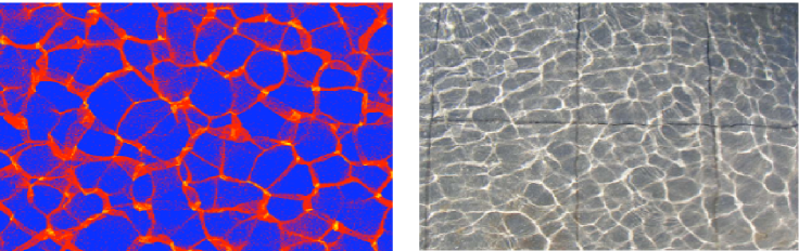
Figure 2: a The distribution of particles in a turbulent flow can show singularities which result from the projection of folded manifolds in phase space: this is a simulation of a two-dimensional compressible flow, taken from [14]. b The singularities are termed caustics, because they have the same structure as singularities in optics. The image (a photograph by Amanda W. Peet) shows a pattern of caustics on the bottom of a swimming pool, resulting from partial focussing of sunlight due to curvature of the water surface by irregular waves. The two images are remarkably similar.

We provide here a critical discussion of results concerning the rate of rain drop and planet formation, which shows that while turbulence can dramatically increase the collision rate, it is not entirely clear whether it is sufficient to explain the coagulation rates observed in nature, and alternative physical explanations may be required.

Over the past few years, the subject of collisions induced by turbulence has received a surge of interest, and as such, it has been the subject of several other review articles, focusing mostly on meteorological applications [15, 16, 6]. This review is more focused on the lessons learned from a general fundamental physics perspective. It is our belief that some of the results shown here will be relevant in other fields of physics, and thus of lasting interest, beyond the specific motivations of the original study.

This article is organised in the following way. In section 2, we review elementary material concerning the motion of particles in a fluid flow, and the collision rate in a suspension, independently of the precise nature of the flow. The more specific aspects of turbulent flows, necessary for the purpose of this review, are discussed in section 3. Section 4 will introduce various mechanisms whereby turbulence can influence the collision rate, including particle clustering and the effects of caustics forming in the phase space of the suspended particles. These diverse contributions to the collision rate are synthesised into a unified approximation scheme in section 5, which is shown to provide a very accurate description of the results of numerical simulation. Having discussed the determination for collision rates we turn to discussion of applications. Section 6 considers the question of whether aerosols undergo a gelation transition, and whether the Smoluchowski equation provides an appropriate description. Sections 7 and 8 consider applications to rainfall and planet formation. In both cases we argue that the insights from considering turbulent enhancement of collision rates do not appear to be sufficient to resolve all of the problems with understanding these processes. The prospects for further developments are considered in section 9, which is our conclusion. A detailed analysis of both fractal clustering and caustics, which are crucial to the determination of the collision rate, is provided in the case of a solvable one-dimensional model in Appendix A (Section 10).

2 Definitions and equations

2.1 Particle motion in a fluid flow

The determination of the motion of particles, even in simple (laminar) flow configurations, is a difficult task. In the applications we have in mind, particles have small sizes, and this leads to a solvable problem. In this limit, the flow can be approximated as constant over a domain much larger than the particle, and the Reynolds number of the particle is so small that the nonlinear term in the Navier-Stokes equations drops out, so the problem can be explicitly solved [17, 18]. The equations of motion involve several terms, which result from the viscous drag of the particle, the gravitational settling, pressure effect, the so-called added mass, and an history (Basset-Boussinesq) force.

Rain drops in a cloud or particles in the interstellar medium have densities, $\rho_{\rm p}$, which are much larger than the fluid density, $\rho_{\rm f}$: $\rho_{\rm p}/\rho_{\rm f}\gg 1$. The resulting inertia of the particles may be large enough to prevent them from exactly following the flow. In this limit, it has been demonstrated [19] that the two dominant forces on small particles are due to viscous drag, which causes the particle velocity to relax towards that of the fluid, and to gravitational settling. The equations of motion for small spherical particles of radius $a$ are determined by Stokes’ formula, so that the equation of motion is

$$\dot{\mbox{\boldmath$r$}}=\mbox{\boldmath$v$}\ ,\ \ \ \dot{\mbox{\boldmath$v$}}=\frac{1}{\tau_{\rm p}}[\mbox{\boldmath$u$}(\mbox{\boldmath$r$},t)-\mbox{\boldmath$v$}]+\mbox{\boldmath$g$}$$ (1)

where

$$\tau_{\rm p}=\frac{2}{9}\frac{a^{2}}{\nu}\frac{\rho_{\rm p}}{\rho_{\rm f}}$$ (2)

is the particle relaxation time, determined from Stokes’ formula for the drag on a moving sphere (in (2), $\nu$ is the kinematic viscosity). The equations of motion (1,2) are valid only in the limit where the suspended particles are very small and very dense: $\rho_{\rm p}/\rho_{\rm f}\gg 1$. When the ratio $\rho_{\rm p}/\rho_{\rm f}$ is smaller than $\sim 10$, the history force becomes important [20]. In cases where a droplet moves through a fluid which has a comparable viscosity, equation (2) must be modified [21, 22].

In astrophysical applications, the gas phase may have extremely low density, so that the size of the aerosol particles may be much smaller than the mean free path of the gas. In this case equation (1) still provides an accurate description of the motion, but the relaxation time $\tau_{\rm p}$ is given by a different expression:

$$\tau_{\rm p}=K_{\rm E}\frac{a\rho_{\rm p}}{c_{\rm s}\rho_{\rm g}}$$ (3)

where $c_{\rm s}$ is the velocity of sound in the gas with density $\rho_{\rm g}$, and $K_{\rm E}$ is a dimensionless constant which is of order unity [23]. The value of $K_{\rm E}$ depends on assumptions about the energy transferred when a gas molecule collides with the surface of the particle.

Describing the motion of larger particles in a turbulent flow remains an outstanding challenge, whose numerical and experimental study is at an early stage [24, 25, 26, 27, 28].

2.2 Collision rates

In principle, the calculation of the collision rate appears to be a straightforward exercise in elementary kinetic theory [29], but in practice it is a surprisingly complex problem. Before discussing the details, it is necessary to consider some fundamental definitions.

Our objective is to quantify the rate $R$ for collision of a given particle with any other particle in the suspension. This quantity is expected to be a function of the radius $a$ of the particle concerned, so our objective is to calculate $R(a)$, which has dimensions of inverse time: $[R]={\rm T}^{-1}$. The rate of collision is expected to be proportional to the number density of particles in the suspension. Let $N(a)~{}\delta a$ be the number density of spherical particles with radius in the small interval $[a,a+\delta a]$. The rate of collisions may be written

$$R(a)=\int_{0}^{\infty}{\rm d}a^{\prime}\ \Gamma(a,a^{\prime})\,N(a^{\prime})$$ (4)

where $\Gamma(a,a^{\prime})$ is a characteristic property of the fluid motion, which is termed the collision kernel. Thus, the specific problem of determining the collision rate $R(a)$ in a given suspension is solved by determining the collision kernel $\Gamma(a,a^{\prime})$, which is independent of the particle density, and then applying equation (4).

The collision kernel may be expressed in terms of other variables, for example when we formulate the Smoluchowski equations in section 6 it will be useful to represent the particle size distribution in term of masses, so that the number density of particles in the interval $[m,m+\delta m]$ is $\bar{N}(m)\,\delta m$. In this case equation (4) is replaced by

$$R(m)=\int_{0}^{\infty}{\rm d}m^{\prime}\ K(m,m^{\prime})\,\bar{N}(m^{\prime})$$ (5)

where $K(m,m^{\prime})$ is collision kernel expressed in terms of mass.

In a monodisperse suspension, where the particles all have approximately the same radius $a$, and where their number density is $n$, equation (4) reduces to:

$$R=\Gamma(a,a)\,n$$ (6)

where

$$n=\int_{0}^{\infty}{\rm d}a\ N(a)=\int_{0}^{\infty}{\rm d}m\ \bar{N}(m)$$ (7)

is the number density of particles.

The collision rate between particles, which are assumed to be spherical, is the rate at which the separation vector between the centres of the particles cross a sphere of radius $a_{1}+a_{2}$, as illustrated in figure 3. Thus, the collision kernel is expected to be proportional to the area of the spherical surface, $4\pi(a_{1}+a_{2})^{2}$. It is also proportional to a suitably defined average of the relative velocity of particles on the sphere of radius $a_{1}+a_{2}$, which will be denoted by $\langle|\Delta v|\rangle$. Also, if the particles have a tendency to cluster together, the collision kernel would be proportional to the two-point correlation function ${\cal C}(r)$ for particles with separation $r=a_{1}+a_{2}$. Putting these factors together, the collision kernel can be written in the form

$$\Gamma_{1,2}=\frac{1}{2}\,4\pi\,(a_{1}+a_{2})^{2}\,{\cal C}(a_{1}+a_{2})\,\langle|\Delta v|\rangle\ .$$ (8)

The factor $\frac{1}{2}$ in (8) is included because only half of the particles crossing the surface are travelling inwards, but this is really just a matter of convention in the definition of $\langle|\Delta v|\rangle$. With a suitable definition of $\langle|\Delta v|\rangle$, this can be presented as an exact equation, see [30, 31].

The collision kernel in (8) depends on the mean relative velocity of the particles, $\langle|\Delta v|\rangle$, which is difficult to calculate. The complex problem of determining the relative velocity between small particles is simply tractable in two limits, relevant to the problem studied here. One case is where the relative velocities might be approximately independent of the separation of the particles, as illustrated in figure 4(a). This is only possible when the particles are able to move relative to the fluid. The other limiting case is where the particles are advected with the fluid. For very small advected particles, their relative velocity at collision $\Delta\mbox{\boldmath$v$}$ is proportional to their separation $\Delta\mbox{\boldmath$x$}$:

$$\Delta\mbox{\boldmath$v$}={\bf A}\,\Delta\mbox{\boldmath$x$}$$ (9)

where ${\bf A}$ is the matrix of velocity gradients, with elements $A_{ij}=\frac{\partial u_{i}}{\partial x_{j}}$.

The approach discussed here is purely geometric, and misses important effects. When two particles get close to each other, the fluid trapped between them leads to a lubrication film, which potentially significantly reduce the collision rates. This reduction can be taken into account by introducing a collision efficiency [2, 32]. It will be discussed in Section 6.1.

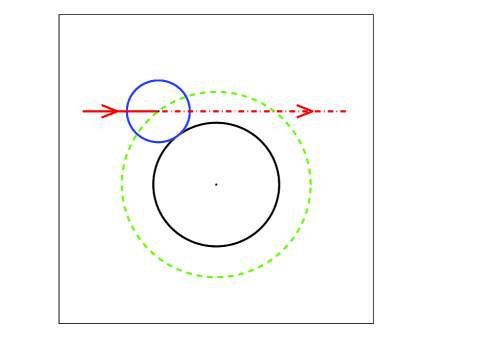
Figure 3: The rate of collision between particles of radius $a_{1}$ and $a_{2}$ is determined by integrating the relative velocity over a spherical surface of radius $a_{1}+a_{2}$, indicated by a dotted line.

Figure 4: The relative velocity of particles might be independent of their separation, illustrated in (a) for a larger particle overtaking a smaller one as they both fall under gravity. Alternatively, the relative velocity may be proportional to their velocity gradient: (b) shows a collision induced by a simple shear flow (in both cases the arrows indicate the velocity of the smaller particle relative to the larger one).

In the following, we discuss three useful examples of physical situations, amenable to an explicit determination of the collision kernel.

2.2.1 Collision in a gas of particles with a Gaussian distribution of velocity

For future reference, we estimate here the collision rate between particles spatially uniformly distributed in a fluid, with statistically independent Gaussian (Maxwellian) distribution of velocities, such that $\langle\mbox{\boldmath$v$}\rangle=0$ and a variance $\langle\mbox{\boldmath$v$}^{2}\rangle_{a}$, which depends a-priori on the radius $a$ of the particles. The assumption that particles are uniformly distributed ensures that ${\cal C}(a_{1}+a_{2})=1$. Assuming that the distribution of the velocity for particle $i$ is $P(\mbox{\boldmath$v$}_{i})=(\frac{3}{2\pi\langle\mbox{\boldmath$v$}^{2}\rangle_{a_{i}}})^{3/2}\exp[-3{\mbox{\boldmath$v$}_{i}}^{2}/(2\langle\mbox{\boldmath$v$}^{2}\rangle_{a_{i}})]$, an elementary calculation shows that the average velocity required in (8) is $\langle|\Delta v_{r}|\rangle=[\frac{2}{\pi}(\langle\mbox{\boldmath$v$}^{2}\rangle_{a_{1}}+\langle\mbox{\boldmath$v$}^{2}\rangle_{a_{2}})]^{1/2}$. This leads to the following collision rate in a suspensions of particles with a Gaussian distribution of velocities:

$$\Gamma_{1,2}=(\frac{8\pi}{3})^{1/2}(a_{1}+a_{2})^{2}[\langle\mbox{\boldmath$v$}^{2}\rangle_{a_{1}}+\langle\mbox{\boldmath$v$}^{2}\rangle_{a_{2}}]^{1/2}$$ (10)

consistent with classical estimates [33].

2.2.2 Collision between settling droplets in still air

We consider now the case of polydisperse suspension of water droplets settling in still air. Integrating (1), and taking into account the dependence on the size $a$ of $\tau_{p}$ leads to the following equations for the settling velocity $\mbox{\boldmath$v$}_{s}$:

$$\mbox{\boldmath$v$}_{s}=-v_{s}\hat{e}_{z},~{}v_{s}=\kappa a^{2}\ ,\ \ \ \kappa=\frac{2}{9}\frac{\rho_{\rm p}}{\rho_{\rm g}}\frac{g}{\nu}\ .$$ (11)

This assumes that the Reynolds number based upon the particle size is small, which is valid for the microscopic water droplets in clouds [32]. Equation (11) shows a strong dependence of $v_{s}$ on $a$: large particles settle much faster than smaller ones. Consider the collision rate between particles of sizes $a_{1}$ and $a_{2}$. In this case, the value of ${\cal C}(a_{1}+a_{2})$ reduces to $1$, and a simple calculation leads to $\langle|\Delta v_{r}|\rangle=\kappa|a_{1}^{2}-a_{2}^{2}|/2$, which immediately leads to:

$$\Gamma_{1,2}=\pi\kappa(a_{1}+a_{2})^{2}|a_{1}^{2}-a_{2}^{2}|\ .$$ (12)

This expression, which grows as a power $\propto a_{1}^{4}$, when $a_{1}\gg a_{2}$, i.e., with a power $4/3$ of the volume of the larger particles, implies that the collision rate of large particles grows very rapidly as their size increases. This fast growth will have an important consequence when studying the problem of coagulation, see Section 6.

2.2.3 Collision in a simple shear flow

Whereas in the two previous examples, the motion of the fluid was not playing any role, consider now a suspension of particles simply transported in a simple (laminar) shear flow: $\mbox{\boldmath$u$}=S(y,0,0)$, so particles are moving in the $x$-direction, with a velocity $\mbox{\boldmath$v$}=\mbox{\boldmath$u$}$, which depends only on its $y$-component (see figure 4). This problem was first treated by Smoluchowski [12]. Once again, assuming a uniform distribution of particles in the flow implies that ${\cal C}(a_{1}+a_{2})=1$. An elementary estimate of the $\Delta v_{r}$ leads to the following expression for $\langle|\Delta v_{r}|\rangle=\frac{8}{3}|S|(a_{1}+a_{2})$, which leads to the collision rate:

$$\Gamma_{1,2}=\frac{16\pi}{3}\,|S|\,(a_{1}+a_{2})^{3}\ .$$ (13)

The collision rate, which is proportional to the shear rate, $S$, and the distance $(a_{1}+a_{2})$ to the third power, is characteristic of the collision rates obtained as a result of shearing motion, at least when the particles follow the flow. In this case, the simple flow structure appears through the shear rate, $S$.

In turbulent flows, velocity differences are created at many scales, generating, among other things, strong shearing motions on small scales. The velocity gradient in turbulence or other complex flow field is described by a real-valued $3\times 3$ matrix ${\bf A}$, which is generically not a simple shear. Other possibilities include the case of locally hyperbolic flow, as illustrated in figure 5. To gain further insight on the statistics of $\langle|\Delta v|\rangle$ requires a more precise description of the properties of the turbulent velocity field, which will be considered in the next section.

Figure 5: The velocity gradient is not usually a simple shear. A locally hyperbolic relative velocity also induces collisions.

3 Elementary properties of turbulent flows

The enhancement of the collision rate by a simple flow, such as a shear flow considered in the previous subsection, provides the first hint concerning enhancement of collision rates by turbulent flows. In fact, significant velocity gradients are ubiquitous in turbulent flows. This section is aimed at providing an elementary discussion of the properties of turbulence relevant to the present discussion.

In this review, we are concerned with turbulence in an incompressible, Newtonian fluid, described by the Navier-Stokes equations:

$$\partial_{t} \mbox{\boldmath$u$}+(\mbox{\boldmath$u$}\cdot\nabla)\mbox{\boldmath$u$}=-\frac{1}{\rho_{\rm f}}\nabla p+\nu\nabla^{2}\mbox{\boldmath$u$}+\mbox{\boldmath$f$}$$ (14)

$$\nabla\cdot \mbox{\boldmath$u$}=0\ .$$ (15)

where $p$ is pressure. The viscous term dissipates kinetic energy in the fluid, so in the absence of any forcing, $\mbox{\boldmath$f$}=0$, the motion simply decays. The Reynolds number, defined as ${\rm Re}=UL/\nu$, where $U$ and $L$ are the velocity and length scales at which the fluid is forced, measures the ratio between the nonlinear term, $(\mbox{\boldmath$u$}\cdot\nabla)\mbox{\boldmath$u$}$ and the viscous (dissipative) term, $\nu\nabla^{2}\mbox{\boldmath$u$}$. In turbulent flows, the Reynolds number is effectively a measure of the intensity of turbulence: turbulence is expected to occur whenever the Reynolds number is very large: ${\rm Re}\gg 1$. Thus, the statement ${\rm Re}\gg 1$ effectively means that, at the forcing scale, viscous dissipation does not play much role. Primarily because the kinematic viscosity $\nu$ is a small quantity, very large Reynolds numbers are common: for example, a convective instability of the atmosphere can create a flow with ${\rm Re}>10^{8}$.

3.1 Scales in a turbulent flow

Turbulence is a notoriously difficult problem [34] but we argue that most of what we need to know can be surmised from dimensional considerations. Kolmogorov [35, 36] introduced the powerful notion that the small structures of the flow have very little ‘memory’ of how the flow was generated. He argued that only one quantity, the rate of kinetic energy dissipation per unit mass, $\epsilon$, is required to characterise fully developed steady and homogeneous turbulent motion over a wide range of length scales (termed the ‘inertial range’ in the turbulence literature). The quantity $\epsilon$, the power dissipated per unit mass, and designated in the following in short as ‘energy dissipation’, is determined by the manner in which the turbulence is generated, by means of large scale flows with characteristic length scale $L$ and velocity scale $U$. Dimensional considerations imply that $\epsilon\sim U^{3}/L$. In the inertial range of length scales, where $\epsilon$ is the only relevant parameter, statistics of the flow can be determined by dimensional analysis. For example, in the inertial range of separations, the variance of the velocity difference between two points depends only upon the separation $R=|\mbox{\boldmath$R$}|$ and the kinematic viscosity $\nu$. Dimensional consistency then implies that

$$\langle[\mbox{\boldmath$u$}(\mbox{\boldmath$R$},t)-\mbox{\boldmath$u$}({\bf 0},t)]^{2}\rangle=C\left(\epsilon|\mbox{\boldmath$R$}|\right)^{2/3}$$ (16)

where the brackets in (16) refer to an average over many flow realizations, and $C$ is a universal dimensionless coefficient.

The turbulence generates successively finer scale eddies until the structures become so small that gradients increase, making the power dissipated per unit mass, $\epsilon\sim\nu\mbox{\boldmath$u$}\cdot\nabla^{2}\mbox{\boldmath$u$}$, significant. The smallest scale reached by the flow is the ‘Kolmogorov lengthscale’, $\eta$, with a characteristic time scale known as the Kolmogorov timescale, $\tau_{K}$. These quantities depend only on $\epsilon$ and $\nu$. Dimensional considerations then imply that

$$\eta=(\nu^{3}/\epsilon)^{1/4}\ ,\ \ \ \tau_{K}=(\nu/\epsilon)^{1/2}\ .$$ (17)

As finer scales are generated by the flow, it is expected that the statistical properties of the flow become homogeneous and isotropic [35, 36]. In this case the kinetic energy dissipation can be obtained directly from (14):

$$\epsilon=\nu\sum_{i,j}\langle A_{ij}^{2}\rangle$$ (18)

where $A_{ij}$, the velocity gradient, is defined by (9). This implies that the typical size of the velocity gradient is the inverse of the Kolmogorov time: $\partial u/\partial x\sim\tau_{\rm K}^{-1}$.

3.2 Velocity gradient statistics

In turbulent flows, the relative motion of two small particles approaching (colliding with) each other is ultimately dominated by the velocity gradient tensor, $\mathbf{A}$, as explained in Subsection 2.2. For this reason, we briefly discuss some elementary statistical properties of the velocity gradient.

The isotropy of the flow imposes that the tensor $\langle A_{ij}(\mbox{\boldmath$x$})A_{kl}(\mbox{\boldmath$x$})\rangle$ is expressible in terms of Kronecker $\delta$ tensors. Using the incompressibility condition ${\rm tr}(\mathbf{A})=0$, as well as relation (18) leads to the following expression for $\langle A_{ij}(\mbox{\boldmath$x$})A_{kl}(\mbox{\boldmath$x$})\rangle$:

$$\langle A_{ij}(\mbox{\boldmath$x$})A_{kl}(\mbox{\boldmath$x$})\rangle=\frac{\epsilon}{30\nu}\Bigl{(}4\delta_{ik}\delta_{jl}-\delta_{il}\delta_{jk}-\delta_{ij}\delta_{kl}\Bigr{)}\ .$$ (19)

Such an estimate is crucial in establishing elementary results, such as the Saffman-Turner collision rate, Eq. (25).

As a particle is transported by the flow, the strain and the vorticity along its trajectory decorrelate with a correlation time of the order of $\tau_{K}$ [37, 38].

3.3 The Stokes number

Comparing the Kolmogorov time $\tau_{\rm K}$ with the response time of the particles, $\tau_{\rm p}$, provides a way to quantify the effect of inertia. This motivates the definition of the Stokes number:

$${\rm St}=\frac{\tau_{\rm p}}{\tau_{\rm K}}\ .$$ (20)

For ${\rm St}\ll 1$, particles are advected by the fluid, and collisions are the result of the shear (the relative motion). When ${\rm St}\gg 1$, the inertia of the particles allows them to move relative to the surrounding fluid, thus leading to entirely different phenomena. The Stokes number is the single dimensionless parameter which distinguishes different physical regimes of the collision process.

3.4 Experimental and numerical investigations

3.4.1 Experimental studies

Despite the vast literature devoted to the experimental investigation of turbulence, very little is known experimentally concerning collisions of particles suspended in turbulent flows.

The investigation of turbulent flows has rested for a long time on methods, such as hot-wire anemometry, which provide only information on the velocity and its spatial correlation function. Over the past decade, new methods have been developed, based on following particles in a turbulent flows using fast-imaging [39, 40]. This has led to a wealth of new information on the motion of particles in a turbulent flows [40]. Although in principle feasible, detecting collisions between small particles in a well-controlled laboratory flow has so far not been possible. It is to be expected that this problem will be solved in a near future. Labelling liquid droplets with chemicals that produce an optically detectable reaction product when the droplets coalesce is a promising approach.

3.4.2 Numerical investigations

The difficulty in obtaining experimental results on collisions in turbulence makes numerical investigations an essential tool. The investigation of fundamental issues in turbulence rests on direct integration of the Navier-Stokes equation, (14) and (15), in a triply periodic domain (effectively a torus) [41, 42, 43]. In such a configuration, the Navier-Stokes can be efficiently integrated using pseudo-spectral methods, based on a (truncated) Fourier series decompositions of the velocity field $u$. For efficiency purposes, the calculation of the nonlinear term $(\mbox{\boldmath$u$}\cdot\nabla)\mbox{\boldmath$u$}$ is carried out in real space, using fast-Fourier methods to transform between real-space and Fourier representations.

Once a solution of the Navier-Stokes equations is determined, the motion of particles, (1), can be efficiently solved [44], permitting to detect collisions [45]. The available computer resources permit to address most aspects of particle collisions.

4 Effect of turbulence on the collision rate

One may think that the effect of turbulence reduces to an effective ‘rate of strain’. The result is more complicated, and much more interesting, as discussed in this section. In the following we describe various effects which become significant as the Stokes number is increased. In the following sections, we focus on the case of monodisperse suspensions, and discuss the collision rate $R$ per particle.

As well as influencing the settling of particles from a fluid suspension by facilitating collisions and aggregation, turbulent motion can have a direct effect upon the settling rate of heavy particles [46]. These single-particle effects are usually less significant than the collisional processes which are the focus of this review.

4.1 The Saffman-Turner limit

Particles with a sufficiently small inertia (small Stokes numbers) essentially follow the flow (independent of their shape or material density). In this case, the velocity gradients generated by turbulence strongly enhance the relative motion between particles, therefore enhancing the chance of collisions, by the mechanism shown in the simple example treated in 2.2.3. A formula derived by Saffman and Turner [8], equation (25) below, determines the collision rate in the small Stokes number case, in the case where the particles are spherical. Two small particles of radius $a$ advected by the flow collide if their separation falls below $2a$. In the case of a suspension of particles uniformly distributed throughout the fluid with density $n$, the rate of collision $R$ for a single particle is obtained, in the spirit of (8), by integrating the relative radial velocity $\Delta v_{r}$ over the surface of a sphere of radius $2a$:

$$R=\frac{1}{2}n\int{\rm d}\mbox{\boldmath$S$}\cdot|\Delta v_{r}|\ .$$ (21)

In this case the relative velocity is determined by the linearisation of the flow field, so that the relative motion of two particles may be described by a hyperbolic velocity field, such as that illustrated in figure 5. The factor of $\frac{1}{2}$ in (21) is required because only half of the sphere where the relative velocity is negative contributes to the collision rate (the overall flux is zero, due to incompressibility). If the particles are small compared to the Kolmogorov length of the flow, the relative velocity resulting from the action of the local velocity gradient $\mathbf{A}$ is given by Eq. (9). Using the explicit expression $A_{ij}=\partial u_{i}/\partial x_{j}$ leads to the following expression for the velocity gradient:

$$\langle|\Delta v_{r}|\rangle=2a~{}\langle|\mathbf{n}\cdot\mathbf{A}\cdot\mathbf{n}|\rangle$$ (22)

where $\mathbf{n}$ is an arbitrary unit vector on the unit sphere. Because of the isotropy of the velocity field, we have

$$\langle|\mathbf{n}\cdot\mathbf{A}\cdot\mathbf{n}|\rangle=\langle\left|\frac{\partial u_{x}}{\partial x}\right|\rangle\ .$$ (23)

This leads to:

$$R=2\pi(2a)^{3}n\langle\left|\frac{\partial u_{x}}{\partial x}\right|\rangle\ .$$ (24)

In order to estimate the expectation value of the partial derivative $|\partial u_{x}/\partial x|$ we assume that the elements of ${\bf A}$ are Gaussian distributed, and note that the variance of $\partial u_{x}/\partial x$ is given by $\epsilon/15\nu$ (see equation (19)). The averaged value is equal to the inverse of the Kolmogorov time scale, up to numerical prefactors [8], leading to:

$$R=\sqrt{\frac{8\pi}{15}}\frac{n(2a)^{3}}{\tau_{\rm K}}\ .$$ (25)

This estimate of the collision rate is based on the only assumption that particles are uniformly distributed, and can be easily extended to suspensions of particles with a dispersion of size [8].

4.2 Clustering in turbulent flows

When the effects of inertia become sufficiently large, i.e., when ${\rm St}$ is large enough, other effects arise, and the collision rate cannot be simply understood in terms of relative motion in the fluid. At finite ${\rm St}$ it is known that particles can show a pronounced clustering. We assume here that the local particle density remains small enough, to prevent feedback from the particles on the flow.

4.2.1 Clustering and the centrifuge effect

Particle clustering is expected to increase the collision rate. The effect of clustering is often ascribed to particles being expelled from vortices by centrifugal action, as proposed by Maxey [47], based on the following argument. Integration of the equation of motion (1) gives

$$\mbox{\boldmath$v$}(t)=\int_{-\infty}^{t}{\rm d}t^{\prime}\ \mbox{\boldmath$u$}(\mbox{\boldmath$x$}(t^{\prime}),t^{\prime})\,\exp[-(t-t^{\prime})/\tau_{\rm p}]\ .$$ (26)

The expression (26) reduces, in the case where $\tau_{\rm p}$ is small, to:

$$\mbox{\boldmath$v$}=\mbox{\boldmath$u$}(\mbox{\boldmath$x$}(t),t)-\tau_{\rm p}\frac{{\rm D}\mbox{\boldmath$u$}}{{\rm D}t}(\mbox{\boldmath$x$}(t),t)$$ (27)

where ${\rm D}/{\rm D}t=\partial/\partial t+\mbox{\boldmath$u$}\cdot\mbox{\boldmath$\nabla$}$. The important remark is that the velocity field $v$, which transports the particles, differs in an essential way from the flow velocity field, $u$: $v$ is effectively compressible, with a divergence

$$\mbox{\boldmath$\nabla$}\cdot\mbox{\boldmath$v$}=-\tau_{\rm p}\sum_{ij}\left(\frac{\partial u_{i}}{\partial x_{j}}\frac{\partial u_{j}}{\partial x_{i}}\right)=-\tau_{\rm p}{\rm tr}({\bf A}^{2})$$ (28)

where ${\bf A}$ is the velocity gradient tensor. Expressing ${\bf A}={\bf E}+\mbox{\boldmath$\Omega$}$, where ${\bf E}^{\rm T}={\bf E}$ is the strain rate tensor (symmetric) and $\mbox{\boldmath$\Omega$}^{\rm T}=-\mbox{\boldmath$\Omega$}$ is the vorticity tensor (antisymmetric) leads to:

$$\mbox{\boldmath$\nabla$}\cdot\mbox{\boldmath$v$}=-\tau_{\rm p}\left[{\rm tr}({\bf E}^{2})-\frac{1}{2}\mbox{\boldmath$\omega$}\cdot\mbox{\boldmath$\omega$}\right]$$ (29)

where $\omega$ is the axial vorticity vector corresponding to the antisymmetric tensor $\Omega$, so that the particle flow is contracting in regions of high strain and expanding in regions of high vorticity. Numerical evidence of a negative correlation between particle density and vorticity when ${\rm St}\approx 1$, as predicted by the ‘centrifuge’ argument has been found numerically [48]. We stress that depends upon making the approximation that $\tau_{\rm p}$ is small. Using (29) provides to a method, valid in the limit of small Stokes number, to analyse clustering [49, 50, 51].

4.2.2 Clustering as a manifestation of a fractal distribution

Figure 1 illustrates the type of clustering phenomena which can occur in turbulent flows. The clustering effect is much stronger than the simple ‘centrifuge effect’ argument suggests, and the positions where the greatest enhancement of density will occur are not predicted by that argument. In reality, the clusters have fractal properties, which should be quantified to determine their influence on collision rates. One way of characterising the fractal distribution of particles is via the correlation dimension [52, 53]. To define this, pick a particle at random, and determine the number ${\cal N}(\epsilon)$ of other particles within a ball of radius $\epsilon$ centred on this particle. The set can be characterised by averaging ${\cal N}(\epsilon)$. The quantity is related to the pair correlation function ${\cal C}(\epsilon)$ of the particle distribution:

$${\cal C}(\epsilon)=\frac{1}{4\pi n\epsilon^{2}}\frac{{\rm d}\langle{\cal N}\rangle}{{\rm d}\epsilon}\bigg{|}_{\epsilon}\ .$$ (30)

If the particle positions sample a fractal measure, it is expected that $\langle{\cal N}\rangle(\epsilon)$ has a power-law dependence:

$$\langle{\cal N}(\epsilon)\rangle\sim n\eta^{3}\left(\frac{\epsilon}{\eta}\right)^{D_{2}}$$ (31)

where $D_{2}$ is the correlation dimension of the set. This implies that the pair correlation function is

$${\cal C}(\Delta r)\sim\left(\frac{\Delta r}{\eta}\right)^{D_{2}-3}$$ (32)

The existence of a fractal measure is implied by very general arguments from dynamical systems theory [52, 53, 54, 55]. The difference between the dimension of the attractor, $D_{2}$, and the dimension of space, $d=3$, is sometimes termed the dimension deficit. This quantity has been investigated numerically, and found to be a function of the Stokes number, reaching a maximum value of approximately $3-D_{2}\approx 0.7$ at ${\rm St}\approx 0.7$ [56]. The effect of particle clustering is argued to enhance the particle collision rate (25) by a factor ${\cal C}(2a)$ (which is large compared to unity when $a\ll\eta$, see Section 5.2 for more precise estimates). As well as numerical investigations, it is also possible to apply analytical techniques to calculate fractal dimensions [57, 58].

We mention here that alternative methods have been proposed to characterize clustering [59, 60].

4.3 Caustics

When inertial effects are more significant, particles can move independently of the fluid, and thus collide with a large relative velocity with other particles. As we explain here, this implies the existence of singularities in the phase-space of the suspended particles which are analogous to ‘caustics’ in optics. These caustics can lead to a pronounced increase in the collision rate as the Stokes number increases. It was realized [50] that when inertia is large enough, particles ejected from vortices acquire velocities which can be very different from the fluid velocity, hence run into other particles with large relative velocity $\Delta v$. This was termed the ‘sling effect’ [50]. Later the phenomenon was described in geometric terms, using the known notion of caustics [14], which provides a convenient framework for understanding and generalisation (caustic structures had been observed earlier in models of particle suspension [61]). Another way to discuss the phenomenon has been proposed in [62, 63, 64].

In order to explain the role of caustics, consider a one-dimensional model, with a fluid velocity $u(x,t)$, and where virtual particles, which are free to pass through each other, evolve with velocity $v$ according to (1). Consider a cloud of particles which are initially on a manifold in this phase space (see figure 6(a)). In the case of particles of negligible inertia, the velocity $v$ of particles remains in the neighborhood of ${u}(x,t)$, so the velocity difference between two closely separated points remains very small. If the particle inertia is significant, however, the velocity of particles can become multivalued (different values of $v$ at the same position) because faster moving particles can overtake slower ones. This is illustrated in figure 6(b). The points where the projection of the phase space-manifold onto the $x$-axis is singular are the caustic singularities. The caustics are focal points where particles with different velocities are brought together at a single point. They are completely analogous to optical caustics, where light is partially focussed onto a line. Note that caustic singularities are created in pairs, and that between them, the velocity is triple-valued. The existence of finite velocity differences between particles at the same location facilitates collisions.

Figure 6: Phase space for a one-dimensional model: (a) The particles are initially on a manifold with a single-valued velocity (b) If particle inertia is significant, particle positions may cross, because fast particles overtake slower ones. The singularities where $\frac{{\rm d}\dot{x}}{{\rm d}x}$ diverges are termed caustics. Creation of caustics is associated with the velocity becoming multi-valued.

In two dimensions the caustic points are replaced by caustic lines, where the density of particles diverges, illustrated in figure 2. In three dimensions the caustics are sheets. In addition, higher-order singularities of the phase-space manifold, classified using catastrophe theory [65], can also form. For example, pairs of caustics can originate from a cusp singularity.

Caustics can increase the collision rate in two different ways. Firstly, the particle density becomes singular in the vicinity of the caustics at $x_{0}$. If $x_{0}$ is the position of the caustic, the density has a generic divergence of the form $n(x)\sim(x-x_{0})^{-1/2}$ as the caustic is approached from one side (here $x$ is any generic coordinate). Secondly, as already explained, the multivalued character of velocity can greatly enhance the collision rate. The same mechanism has also been discussed in terms of ejection from vortices [50], and termed sling effect. The relations between caustics and collisions of inertial particles were proposed in [14, 66].

The nature of the singularity at caustics can be illuminated by considering the gradient of the velocity for nearby particles. Assuming a continuum fluid description for the flow of particles, and differentiating Eq. (1) leads to the following evolution equation for the tensor $\mathbf{\sigma}$, defined by $\sigma_{ij}\equiv\partial_{i}v_{j}$:

$$\frac{d\mathbf{\sigma}}{dt}+\mathbf{\sigma}^{2}=\frac{1}{\tau_{\rm p}}(\mathbf{A}-\mathbf{\sigma})\ .$$ (33)

where $\mathbf{A}$ is the velocity gradient tensor. Equation (33), whose nonlinearity is of the Burgers type, is a convenient starting point to analyze caustic formation numerically [67] or even experimentally [68].

To estimate the contribution of the caustic mechanism to the collision rate, Eq. (8), we approximate the typical velocity difference associated with the sling effect as $\sim\eta/\tau_{\rm K}$, up to a dimensionless function of ${\rm St}$ and the Reynolds number of the flow, ${\rm Re}$:

$$R=\frac{4\pi a^{2}n\eta}{\tau_{\rm K}}\,F({\rm St},{\rm Re})\ .$$ (34)

The function $F({\rm St},{\rm Re})$ must vanish in the limit as ${\rm St}\to 0$, because the caustic mechanism is absent in the advective limit. In the Appendix it will be argued that ${\rm St}\to 0$ is a singular limit, and that

$$F({\rm St},{\rm Re})\propto\exp(-S/{\rm St})$$ (35)

provides a qualitatively plausible representation, in agreement with numerical estimates [67, 69].

It will be demonstrated later, see Section 5, that the caustic or sling effect provides the dominant contribution to the collision rate, as soon as the inertia becomes significant (for ${\rm St}\gtrsim 0.5$).

4.4 Random uncorrelated motion

In the limiting case where the turbulence intensity is very high, an alternative approach to understanding the effect of increasing the turbulence intensity was initiated by Abrahamson [70]. When the damping timescale $\tau_{\rm p}$ is large, particles travel for long distances through the fluid, without being influenced by the smaller scale turbulent eddies. Abrahamson argued out that this implies that the particles which reach any one point will have approximately isotropic random velocities, so that the gas-kinetic approach described in section 2.2.1 can be used to model the motion of the suspended particles. This point has also been emphasised in [63], where this regime was termed ‘random uncorrelated motion’.

In a turbulent flow there is a largest timescale, $\tau_{L}$ (the integral timescale) which is characteristic of the driving motion which creates the turbulence. Whenever $\tau_{\rm p}\ll\tau_{L}$, the particles will be advected with the largest eddies, and not be sensitive to eddies with a timescale smaller than $\tau_{\rm p}$. The velocity difference $\langle|\Delta v|\rangle$ in Eq. 8 can be estimated as the typical relative velocity of particles at any given point. This is comparable with the relative velocity of the particles and the fluid. We now describe a simple argument which can be used to surmise an expression for the mean magnitude of the relative velocity, $\langle|\Delta v|\rangle$.

We argue, in the spirit of Kolmogorov phenomenological description, that in the inertial range the only parameter which enters the description of the flow is the rate of dissipation per unit mass, $\epsilon$, together with the time scale characteristic of the particle motion, $\tau_{\rm p}$. Dimensional arguments then lead to the following expression for the relative velocity:

$$\langle|\Delta v|\rangle={\cal K}\sqrt{\epsilon\tau_{\rm p}}$$ (36)

where ${\cal K}$ is a dimensionless constant (this approach was developed in [71]). This leads to a formula for the rate of collision in a highly turbulent flow:

$$R\approx K\frac{na^{2}\eta}{\tau_{\rm{}_{K}}}\sqrt{{\rm St}}$$ (37)

The constant $K$, which is potentially important for astrophysical applications, will be discussed in Section 5.2.

5 Synthesis: a unified theory for the collision rate

5.1 Modelling the collision rate

We have discussed several mechanisms for the role of turbulence in facilitating collisions between suspended particles. The shear component of turbulence causes collisions between particles moving with the fluid, at the rate which estimated by Saffman and Turner. In addition, the inertial effects, parametrized by the Stokes number, induce two distinct effects. Firstly, there is the clustering effect known as preferential concentration. Secondly, particles located at the same spatial location may have very different velocities, a consequence of the caustic folds in phase space. Finally, in the limiting case when the inertia is very large, it was argued that the motions of the particles become completely uncorrelated from one another, and a simple asymptotic form for the collision rate was proposed. In this section, we show how to combine these competing mechanisms. The main result of the section is a derivation of a simple expression for the collision rate. It involves some parameters, which must be determined empirically by comparison with simulations. We also consider the evidence supporting our expression coming from numerical simulation as reported in [72].

The central idea is that the collision rate can be resolved into two components. Some collisions arise from particles which follow similar trajectories for an extended period, and which eventually come into contact because of shearing motion in the flow. At low Stokes number, where particles are exactly following by the flow, this is the only mechanism. The collision rate due to this mechanism is denoted $R_{\rm adv}$, and it is controlled by the local shear rate, as well as by the local concentration around particles. Collisions between particles not following fluid path lines, occurring when caustics start to form in the phase-space of the suspended particles, give rise to a very different contribution, denoted here by $R_{\rm caust}$. The two contributions $R_{\rm adv}$ and $R_{\rm caust}$ differ in an essential way by their dependence on the siza $a$ of particles. We argue that these mechanisms operate independently and that their contributions are additive, so that

$$R=R_{\rm adv}+R_{\rm caust}\ .$$ (38)

This decomposition was proposed by analysing theoretical models [66, 73] and simulations of simplified numerical models [69]. There is no hard criterion which distinguishes between an advective and a caustic-mediated collision, so (38) must be regarded as an approximation. In the following, we derive the form of the terms $R_{\rm adv}$ and $R_{\rm caust}$ in (38).

In the limit ${\rm St}\ll 1$ the collision rate is determined by shearing motion, without any inertial effect, and the collision rate is given by equations (25) [8].

The preferential concentration causes clustering of particles with finite values of ${\rm St}$. The density of particles at a distance $r$ from a given test particle is $n{\cal C}(r)$, where ${\cal C}(r)$ is a radial correlation function. An important remark is that the inertial effect that leads to clustering does not enhance significantly the relative velocity of particles, contrary to caustics. In fact, particles with large velocity differences do not stay together, thus not contributing to preferential concentration. As a result, the enhancement of the local concentration around particles contributes only the $R_{\rm adv}$ term, which becomes:

$$R_{\rm adv}=\sqrt{\frac{8\pi}{15}}\frac{n(2a)^{3}}{\tau_{\rm K}}{\cal C}(2a)\ .$$ (39)

When inertial particles converge to a fractal measure, as we have argued, see Section. 4.2), the function ${\cal C}(r)$ behaves as a function of $r$ as a power-law: ${\cal C}(r)\propto r^{-D_{2}-d}$.

In the caustic-dominated case we combine expressions (34), (35) and (37) to obtain an expression for the rate of collisions due to caustics:

$$R_{\rm caust}=K\frac{na^{2}\eta}{\tau_{\rm K}}\sqrt{{\rm St}}\exp(-S/{\rm St})$$ (40)

where $K$ and $S$ are two constants to be determined by fitting the collision rate against numerical simulations: $K$ determines the asymptotic collision rate at very large Stokes numbers, and $S$ determines the crossover point where the caustic mechanism becomes significant. The non-analytic term is consistent with theoretical expectations [66] and numerical studies [67].

Taken together, equations (38)-(40) define the theory for the collision rate. We note that the function $F({\rm St},{\rm Re})$ defined in equation (34) is known only through its asymptotic behaviour in certain regimes, so further information is necessary to make progress. The two terms in (38) differ in an essential way through their dependence on the size of the particles $a$, at a fixed value of ${\rm St}$ and ${\rm Re}$. Namely, $R_{\rm caust}$ varies as $a^{2}$, wheres $R_{\rm adv}$ varies as $a^{D_{2}}$ ($D_{2}>2$). This difference can be used to separate the different contributions numerically. We present in the following section numerical results, which indicates that the decomposition (38) is indeed a very effective tool for the analysis of collision rates. We note that Zaichik and co-workers [74, 75] proposed models of the rate of collision in turbulent flows which use similar physical principles. Their final expressions for the collision rate involve a much larger number of parameters than equations (38)-(40).

As well as the collision rate, the probability distribution of relative velocities of colliding particles is also of interest, especially in the context of understanding planet formation, where collisions may be sufficiently energetic to cause fragmentation [76, 77].

5.2 Numerical evidence on collision rates

A substantial amount of literature has been devoted to the numerical investigation of the collision rates in both direct numerical simulations (DNS) of the Navier-Stokes equations, and model flows, but many of these studies pre-date some of the theoretical insights contained in equations (38)-(40) above. The collision rate does show a marked increase as the effects inertia are increased, and this is usually ascribed to the effects of ‘preferential concentration’, that is the clustering effect, but it has been argued that effects of caustics may also be significant [30]. Here we summarise some recent numerical studies which separate out the two contributions in equation (38) by studying the dependence of the collision rate upon particle size, keeping the Stokes number fixed. This is achieved by varying the ratio of the particle density to the fluid density, $\rho_{\rm p}/\rho_{\rm f}$. Modifying the ratio $\rho_{\rm p}/\rho_{\rm f}$ at fixed value of the Stokes number is achieved by varying in the collision detection algorithm the radius of the particles, $a$, according to (2),(20) (so that $a\propto(\rho_{\rm p}/\rho_{\rm f})^{-1/2}$).

The collision rate, $R$, is determined numerically by recording among a set of trajectories, all instances in which the separation radius decreases past $2a$. In the case of collisions where particles stick or coalesce on contact, we should only count the first contact collisions. This effect should be accounted for by introducing a factor $f<1$ in (38). The coefficient is no smaller than $\approx 0.85$ when ${\rm St}$ is very small, and decreases when ${\rm St}$ increases [78]. Here, we do not distinguish between single and multiple collisions. The collision rate, $R$, shown in Fig. 7(a), is normalized by $n(2a)^{3}/\tau_{\rm K}$ and plotted as a function of ${\rm St}$. The Saffman-Turner prediction, (25), implies that in the limit ${\rm St}\rightarrow 0$, the quantity $R\tau_{\rm K}/(n(2a)^{3})$ should become independent of the ratio $\rho_{\rm p}/\rho_{\rm f}$. Our own numerical results [72], in agreement with other estimates [30, 31], are only consistent with this prediction for small values of ${\rm St}$. Fig. 7(b) shows that $R\tau_{\rm K}/(na^{2}\eta)$ as a function of the Stokes number, does not depend much on $\rho_{\rm p}/\rho_{\rm f}$ for values of ${\rm St}$ larger than $\gtrsim 0.3$. This scaling is consistent with the sling/caustics collision mechanism, described by equation (39). We note that $F({\rm St},{\rm Re})$ deduced from Fig. 7(b) does not fit the asymptotic form $F({\rm St},\infty)=K\sqrt{{\rm St}}$ for large values of ${\rm St}$. We ascribe this to the limited Reynolds number of our numerical simulations.

Figure 7: The collision rate $R$ as a function of the Stokes number ${\rm St}$, for three different values of the ratios of density $\rho_{\rm p}/\rho_{\rm f}=250$, $10^{3}$ and $4\times 10^{3}$. The collision rate $R$ is normalized by $n(2a)^{3}/\tau_{\rm K}$ (a), and $n(2a)^{2}\eta/\tau_{\rm K}$ (b). The horizontal dashed line in (a) corresponds to the Saffman-Turner prediction.

Figure 8 shows the effect of clustering in the same simulations: the effect of clustering on the function ${\cal C}(2a)$ reaches a maximum at a value ${\rm St}\approx 0.7$ of the Stokes number. The collision rate grows much larger at higher values of the Stokes number, which provides further indication that caustic effects dominate the collision rate.

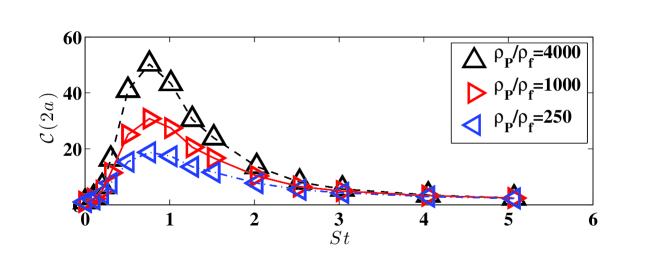
Figure 8: The function ${\cal C}(2a)$ that measures preferential concentration, for three values of the density ratio, $\rho_{\rm f}/\rho_{\rm f}$, as indicated in the figure. The preferential concentration does not play a significant role for ${\rm St}\gtrsim 5$

Figure 9 shows the relative importance of the advective and caustic terms in these simulations. The caustic contribution becomes dominant for Stokes numbers greater than $\approx 0.75$.

Figure 9: The ratio of the contribution to the collision rate due to preferential concentration $R_{\rm adv}$, defined by equation (39) and of the total collision rate, $R$. At fixed value of $\rho_{\rm p}/\rho_{\rm f}$, The contribution of $R_{\rm adv}$ to the total collision rate decreases when the Stokes number increases, or when the ratio $\rho_{\rm p}/\rho_{\rm f}$ increases.

At very large Stokes numbers the collision rate is expected to be given by (37), which is a potentially important prediction for astrophysical applications. To estimate the unknown constant $K$ in (37), one needs simulations at high enough ${\rm St}$, i.e., high enough $\tau_{p}$, but with the constraint that the value of $|\mbox{\boldmath$R$}|$, such that $\tau_{p}=(|\mbox{\boldmath$R$}|^{2}/\epsilon)^{1/3}$, is in the inertial range. Extrapolation of numerical data at moderate Reynolds numbers from different sources [79] leads to a value $K\approx 50$.

An alternative decomposition of the collision rate, originally proposed by [30], expresses the collision rate $R$ as a product in which the term ${\cal C}(2a)$, which describes the local concentration enhancement around a particle, appears as an overall factor:

$$R=2\pi(2a)^{2}n{\cal C}(2a)\langle|\Delta v|\rangle_{\rm eff}$$ (41)

This representation, which is exact for a suitable definition of $\langle|\Delta v|\rangle_{\rm eff}$, suggests that the preferential concentration and sling effects act together to enhance the collision rate. Fig. 7(b) demonstrates that if this parametrisation of the collision rate is used, then the dependence of ${\cal C}(2a)$ upon $\rho_{\rm p}/\rho_{\rm f}$, see Fig. 8 must be cancelled (for ${\rm St}\gtrsim 0.5$) by a reciprocal dependence of the collision velocity, $\langle|\Delta v|\rangle_{\rm eff}$. In fact, previous measurements [80, 81] of the dependence of ${\cal C}(r)$ and of the average velocity difference as a function of $r$ suggest power law dependences, the exponents being such that the product ${\cal C}(2a)\langle|\Delta v|\rangle_{\rm eff}$ is essentially constant for ${\rm St}\gtrsim 0.5$. Equations (38), (39) and (40) provide a very natural explanation of this cancellation. We remark that the power-law dependence of the collision velocity has been explained in a random flow model [73, 82], and used to justify Eq. (38) for that system.

We therefore conclude that the decomposition (38), which rests on a physically well-motivated analysis, and which is supported by the analysis of simplified theoretical models, provides a consistent description of the available numerical data. One of the main lessons from the analysis of the dependence of the collision rate on ${\rm St}$ and on the ratio $\rho_{\rm p}/\rho_{\rm f}$, is that the sling/caustic effect provides the dominant mechanism for the dramatically enhanced collision rate of particles whose Stokes number exceeds $\gtrsim 0.75$, in the cases of water droplets.

6 From collisions to aggregation

Up to this point we have considered expressions for the rate of geometrical collisions. In order to determine the aggregation of particles, we need to consider whether the collisions result in particles combining, and how the population of particle sizes evolves.

6.1 Collision efficiency

Droplets which undergo a geometrical collision, i.e. whose separation falls below $a_{1}+a_{2}$ when their motion is predicted by equation (1), might not coalesce, because the streamlines of small droplets curve around larger ones. In fact, if the Navier-Stokes equations were a complete description, droplets would never collide, because of the presence of a lubricating film of fluid between them. Other mechanisms allow the particles to actually coalesce [83].

The aggregation of particles is characterised by a collision efficiency $e$, defined as the ratio of the observed rate of coalescence to the rate of geometrical collisions (where the separation of the centres predicted by Eq. (1) falls below $a_{1}+a_{2}$). The coalescence efficiencies are hard to determine, because the the complex physics determining breakdown of the lubricating layer. It is widely accepted that they are low for typical cloud droplets [32, 2]. If the larger droplet has radius below $20\,\mu{\rm m}$, it is believed that $e\leq 0.1$, and that for radius $10\,\mu{\rm m}$, $e\leq 0.03$ [2]. For droplets of size $a=50\,\mu{\rm m}$ colliding with droplets of size $a=10\,\mu{\rm m}$, however, the efficiencies are expected to be close to unity [32, 2].

6.2 Models of aggregation

The theory developed by Smoluchowski [12] to describe the coagulation in colloids seems to provide a general framework to discuss a vast class of problem, including coalescence of water [3, 84] or of dust grains. The approach of [12] is naturally formulated in terms of mass conservation, so we use here $\bar{N}(m,t)$ the number of particles of mass $m$ per unit volume at instant $t$. The Smoluchowski equation is:

$$\frac{\partial\bar{N}}{\partial t}(m,t) = \frac{1}{2}\int_{0}^{m}{\rm d}m^{\prime}\ K(m-m^{\prime},m^{\prime})\bar{N}(m^{\prime},t)\bar{N}(m-m^{\prime},t)$$

$$- \bar{N}(m,t)\int_{0}^{\infty}{\rm d}m^{\prime}\ K(m,m^{\prime})\bar{N}(m^{\prime},t)\ .$$

The Smoluchowski description is a mean-field model, in that it assumes that the particle density is spatially uniform. To treat aggregation processes, the Smoluchowski approach is generally preferred to the full master equation, which is completely intractable.

Depending on the structure of the collision kernel $K(m.m^{\prime})$, the Smoluchowski equation can predict one of two different types of particle growth. In ripening processes, the particles grow but they remain of comparable sizes. Alternatively, if the collision kernel $K(m,m^{\prime})$ increases sufficiently rapidly as $m,m^{\prime}\to\infty$, the growth process is unstable: a small fraction of particles undergoes runaway growth in a finite time. This means that, in the Smoluchowski model, all of the smaller particles end up absorbed into one massive cluster in a finite time. This phenomenon, known as gelation, has been investigated intensively: see [13] for a review. In the notation of Eq. (6.2), gelation is expected to happen when the collision rate $K(m,m^{\prime})$ grows faster with $m$ and $m^{\prime}$ than linearly [85]. This is of primary concern in our case, since for large values of the mass, or equivalently, of the radius, the dominant physical effect in the collision rate is due to particle settling, see Eq. (12). In this case, the kernel $K$ grows as $K(M,m)\propto M^{4/3}$ when $M$ is large, so the mean-field equation (6.2) leads to gelation. Here we discuss the consequences of the gelation transition in the Smoluchowski model.

The requirement of a very large number of collisions, of the order of $10^{6}$, to form a raindrop of typical size $1\,{\rm mm}$ out of much smaller microscopic droplets (of typical size $10\,\mu{\rm m}$) makes gelation an appealing feature of the Smoluchowski equations.

There is, however, a potential problem with using the Smoluchowski equation to model rainfall. The gelling transition occurs after a critical time $t_{\rm c}$. Investigations of the gelation transition for the Smoluchowski equation for homogeneous kernels of the form

$$K(m_{1},m_{2})={\rm const.}\ m_{1}^{\mu}m_{2}^{\nu}$$ (43)

have shown rigorously [86, 87] that there is a gelation transition when $\mu+\nu>1$, and that $t_{\rm c}=0$ (termed instantaneous gelation) whenever $\nu>1$ or $\mu>1$. The kernel for liquid droplets settling under gravity is asymptotic (when $m_{1}\gg m_{2}$) to a homogeneous kernel with $\nu=4/3$, so the issue of instantaneous gelation is relevant.

These results suggest that the Smoluchowski equations, which predict an instantaneous gelation, must to be used with caution.

We should consider the reason why the Smoluchowski equation has this pathological behaviour when $\nu>1$. Two observations are necessary to explain the origin of the zero-time singularity. First, note that a cluster of size $M$ will grow to infinite size in a time $t_{\rm c}(M)$, which should be a decreasing function of $M$ (because the rate of collisions is assumed to increase with the cluster size). Furthermore, under the conditions where instantaneous gelation occurs, this time $t_{\rm c}(M)$ approaches zero as $M\to\infty$. The second observation is that, in an infinite system, a cluster of size $M$ arises in a finite time $t_{0}$ somewhere in the system, no matter how small we choose $t_{0}$: we can find a cluster of size $M$ somewhere in an infinite system, no matter how small we make $t_{0}$ or how large we make $M$. According to the Smoluchowski equation, the model thus undergoes gelation at a time $t=t_{0}+t_{\rm c}(M)$ where both $t_{0}$ and $t_{\rm c}$ can be made arbitrarily small. This argument applies to a system with an infinite number of particles: see [88] for a discussion of finite-size effects.

We note that the prediction of a runaway growth may need to be revised, because when the droplets become very large, the terminal velocities are proportional to $a^{1/2}$, so the collision kernel grows as $m^{5/6}$, which does not yield a gelation transition. In addition, rain droplets may undergo fragmentation when they become sufficiently large [89].

This pathology of zero-time gelation results from the use of a mean-field description, which ignores any spatial structure of the particle density ${\bar{N}}(m,t)$. Under the mean-field approximation, the local depletion of particles due to the formation of a large cluster is not taken into account, so an unbounded growth can proceed. We conclude that the Smoluchowski equation must be used caution, and that a proper description of the runaway growth therefore requires more realistic assumptions about the spatial distribution.

7 Application to rain initiation

The problem we are focusing on here concerns the generation of rain drops in ‘warm’ (ice-free) cumulus clouds [32, 2, 90, 3]. In ice-bearing clouds the Wegener-Bergeron-Findeisen can result in rapid growth of ice crystals by condensation, which makes it easier to explain precipitation [32]. When the air becomes supersaturated, water droplets condense rapidly onto aerosol nuclei. They grow up to a typical radius $10\,\mu{\rm m}$ before the supply of water vapour is exhausted. The later stages of the growth of a raindrop (from radius of approximately $50\,\mu{\rm m}$ upwards) involve the falling drop growing rapidly by coalescence with microscopic droplets lying in its path, and are easier to understand. The challenge is to explain the growth of droplets from size $10\,\mu{\rm m}$ to approximately $50\,\mu{\rm m}$, and in particular, to identify the physical process leading to the rapid onset of rain showers, which can develop in less than half an hour.

To illustrate the discussion, consider the following representative values for a convecting cumulus cloud which could produce precipitation [32, 3]. The typical droplet radius is $a=10\,\mu{\rm m}$, the number density of droplets is $n=4\times 10^{8}\,{\rm m}^{-3}$, and the cloud depth is $L=10^{3}\,{\rm m}$. The typical vertical velocity of air inside the cloud has magnitude $2\,{\rm m}\,{\rm s}^{-1}$, so that the eddy turnover time may be taken to be $\tau_{L}=10^{3}\,{\rm s}$. An estimate for the rate of dissipation is $\epsilon\approx L^{2}/\tau_{L}^{3}=10^{-3}\,{\rm m}^{2}{\rm s}^{-3}$, which gives an estimate of the Kolmogorov time $\tau_{\rm K}\approx 10^{-1}\,{\rm s}$. Rain falls as droplets of size approximately $1\,{\rm mm}$.

What are the processes possibly leading to the growth of very small droplets with an initial size of typically $10\,\mu{\rm m}$? Growth can proceed by collisions, and one possibility is that droplets settling at different rates lead to collisions. This mechanism is only possible in the presence of size dispersion among droplets. Specifically, inserting values for air and water at $5^{\circ}{\rm C}$ into equation (11) gives $\kappa\approx 1.4\times 10^{8}\,{\rm m}^{-1}{\rm s}^{-1}$. Then, using the expression of the collision rate (12) to estimate the coalescence rate of a droplet of radius $a+\Delta a$ (with $a=10\,\mu{\rm m}$, $\Delta a\approx 2.5\,\mu{\rm m}$) falling through a gas of smaller droplets (of radius $a=10\,\mu{\rm m}$), and with a collision efficiency $e\approx 0.03$, gives a rate of coalescence $R\approx 10^{-4}{\rm s}^{-1}$. We conclude that the rate of coalescence of typical sized water droplets induced by differential settling is very small, as long as the dispersion between particles is small.

As the air in a convecting (cumulus) cloud is turbulent, it may be expected that the coalescence rate between droplets may be greatly facilitated by turbulence [8]. Using the expression for the collision rate between small droplets following the flow, (25), and the parameters of the cloud model, gives $R_{\rm turb}\approx 2\times 10^{-6}\,{\rm s}^{-1}$, which is negligible. The effects of turbulence are dramatically increased when the effects of droplet inertia are significant. Inertial effects are measured by the Stokes number, ${\rm St}\equiv\tau_{\rm p}/\tau_{\rm K}$. The collision rate is greatly enhanced by effects due to caustics for ${\rm St}\gtrsim 0.3$ [72]. With the values of cloud model given above, however, the estimated Stokes number is ${\rm St}\approx 10^{-2}$, which is to small to lead to any significant enhancement.

The small rate of collisional coalescence of droplets is clearly a problem. It should be kept in mind that considerable variation exists among various clouds, and even within a given cloud, the flow is expected to be very inhomogeneous. The numbers used in the estimates above could therefore vary significantly, resulting in a large increase of the coagulation rates, compared to the values given here, at least in parts of the clouds. One may also remark that only a very small proportion of the microscopic droplets needs to be converted into raindrops. Consider the rate at which droplets actually form. Rainfall at a rate of $3.6\,{\rm mm}\,{\rm hr}^{-1}=10^{-6}\,{\rm m}\,{\rm s}^{-1}$ is considered as ‘moderate’ [32]. If the raindrops have size $a\approx 1\,{\rm mm}$, the number of drops falling per second and per square meter is approximately $250$. Given the assumed cloud depth of $L=10^{3}\,{\rm m}$, the volumetric rate of production of raindrops is approximately $0.25\,{\rm m}^{-3}{\rm s}^{-1}$. If the microscopic droplets have density $n=4\times 10^{8}\,{\rm m}^{-3}$, then the rate of conversion of each microscopic droplet into a ‘collector’ droplet undergoing runaway growth is approximately $6\times 10^{-10}\,{\rm s}^{-1}$. Alternatively, during a five minute shower, the probability that a water droplet starts growing, and accumulates during its subsequent fall enough droplets to become a rain droplet is small, approximately $2\times 10^{-7}$. The problem of rain initiation is, therefore, concerned with the frequency of very rare events [91].

Despite the fact that the required conversion probability is very small (of order $10^{-7}$), growth of droplets is too slow by a collisional mechanism. On growing from $10\,\mu{\rm m}$ to $50\,\mu{\rm m}$, the volume of a droplet increases by a factor of $125$, that is, there are or order $100$ collision events. It was argued above that the rate for the first collision events is small, $R\approx 10^{-4}\,{\rm s}^{-1}$. It is not obvious whether the rarity of the event is sufficient to compensate for the low rate of multiple collisions. Large deviation theory (reviewed in [92]) is the appropriate tool for analysing this problem. A large deviation analysis shows that a sufficient number of droplets can undergo runaway growth in small fraction of the mean time to the first collision [93].

After a droplet has grown to a size much larger than the typical droplet size, it falls rapidly and collects other droplets in its path. When $a>50\,\mu{\rm m}$ we assume that the collision efficiency is approximately unity. Consider a droplet of size $a_{1}$ falling through a ‘gas’ of small droplets, which can be characterised by the liquid volume fraction $Q=4\pi n\langle a^{3}\rangle/3$. The large droplet falls with velocity $v=\kappa a_{1}^{2}$ and grows in volume at a rate $\pi a_{1}^{2}Qv$, so that

$$\frac{{\rm d}a_{1}}{{\rm d}t}=\frac{\kappa Qa_{1}^{2}}{4}\ .$$ (44)

Solving this equation shows that the droplet radius diverges in the time

$$\tau_{\rm exp}=\frac{4}{\kappa Qa_{1}}\ .$$ (45)

Equation (45) predicts that the time before runaway increases rapidly as the droplet size decreases. For the parameters introduced to describe a cloud, a droplet of size $a_{1}=50\,\mu{\rm m}$ requires $\tau_{\rm exp}\approx 2\times 10^{3}\,{\rm s}$ to undergo explosive growth.

We conclude that, although runaway growth can proceed when a droplet reaches $50\,\mu{\rm m}$, it is difficult to understand how droplets can reach this size in the short time that it takes for a rain shower to develop. While turbulence mediated collisions may be an important ingredient to explain the runaway growth of rain drops in warm cumulus clouds, a complete picture is likely to involve other effects, possibly including those triggered by non-collisional growth processes [94]. Such effects need to be discussed more systematically in the future.

8 Application to planet formation

The other major area for applications of turbulent collision processes is in understanding planet formation. Here we can only give a brief introduction to a complex and rapidly developing research field. We start by summarising the standard model, which is reviewed in [95], before discussing the unresolved difficulties.

When a star forms by gravitational collapse, conservation of angular momentum prevents all of the cloud of gas from falling into the star, and the residual material rapidly forms a disc-like structure (which has the least internal motion consistent with the conservation of angular momentum). It is assumed that planet formation occurs in such circumstellar discs surrounding young stars [7], which implies that planets would be created with near circular orbits in the plane of the disc. This model is consistent with the structure of the solar system, where the planets lie in approximately circular and coplanar orbits, close to the equatorial plane of the Sun. The structure of these circumstallar discs is described by a model introduced by Shakura and Sunyaev [96].

The interstellar medium from which planets form is thought to contain sub-microscopic dust. The grains have a broad distribution of sizes, but $10^{-7}\,{\rm m}$ is a typical value. The grains may be ice particles or minerals, predominantly silicon or carbon based, originating from nuclear reactions in stars. The proportion of ‘heavier’ elements (that is, elements other than ${\rm H}$ and ${\rm He}$) in star forming regions is of the order of one percent by mass. There is also a consensus that the dust grains play an important role in planet formation. It is assumed that dust grains adhere on contact, making ever larger structures. In the simplest version of this model, these objects continue to accumulate material until they become kilometre-sized ‘planetesimals’, and gravitational forces between the planetesimals take over. A variation on this model suggests that ‘boulders’ settle to form a layer at the mid-plane of the circumstellar disc. When the density of material at the mid-plane reaches a critical level, this triggers a gravitational collapse [97].

Collisions between grains to produce larger structures play an essential role in these routes to planet formation, and the aim is to understand whether a quantitative description of these processes is viable. In addition to the difficulty in estimating the physical parameters inside a circumstellar with current observational techniques, some serious theoretical difficulties with these models are hard to circumvent [98].

In the absence of any turbulent transport mechanism, the rate of collision of microscopic grains is very low. It seems likely, but it is not certain, that the gas in a circumstellar disc is in turbulent motion: the Reynolds numbers associated with the motion are extremely high, and the effects such as convection due to frictional heating will combine with the rotational motion. Turbulence certainly increases the rate of collisions, but it also brings its own problems [99]. The dust particles will adhere to each other due to van der Waals forces and to a certain extent electrostatic forces. Because these binding forces are weak, aggregates of dust particles are very easily fragmented by collisions. Estimates of the relative velocity of particles colliding in a turbulent environment such as equation (36) indicate that the collision speed increases with the size of the particles [9, 71], so that there may be a maximum value for the size of a dust cluster which can be formed by aggregation in a turbulent environment. Recent estimates indicate that the maximum size that can be reached by clusters of dust particles appears to be very small for reasonable values of the parameters in a model for the protoplanetary accretion disc. It is useful to give some estimates for conditions inside the circumstellar disc according to the Shakura-Sunyaev model. These have a power-dependence upon distance from the star, but at $1\,{\rm AU}=1.5\times 10^{11}\,{\rm m}$ (i.e., the Earth-Sun distance) the gas density is $3\times 10^{-4}\,{\rm kg}\,{\rm m}^{-3}$, the dissipation rate is $10^{-3}\,{\rm m^{2}}\,{\rm s}^{-3}$, the gas mean-free-path is $4\times 10^{-3}\,{\rm m}$, the speed of sound is $700\,{\rm m}\,{\rm s}^{-1}$ [98]. The low density of the gas implies that the Epstein formula (3) is applicable, and the particle relaxation time $\tau_{\rm p}$ is very large. Thus, equation (36) implies that the relative velocity of colliding particles is quite large. For example $30\,{\rm cm}$ size objects are predicted to collide with velocities of approximately $10\,{\rm m}\,{\rm s}^{-1}$ [98]. It seems improbable that balls of dust particles would survive collision at these speeds. These considerations suggest that there are severe theoretical difficulties with models based upon aggregation of dust particles.

Other outstanding theoretical difficulties are related to the model itself, and are independent of whether turbulence plays a role in collisional aggregation. One of the difficulties concerns the fact that the gas in an accretion disc is partially supported by its pressure, so that its orbital velocity is slightly lower than the Keplerian value in the quasi-static state. A ‘rock’ (more accurately, an aggregate of dust grains and possibly ices) which is entrained with the gas is not supported by the pressure and consequently slowly spirals in towards the star [100, 101]. This effect is most pronounced for rocks with size comparable to the mean free path of the gas (typically $1\,{\rm cm}$ to $1\,{\rm m}$), and the timescale for spiralling in is of the order of $300\,{\rm yr}$ starting from an orbit at $1\,{\rm AU}$. Even under the most favourable assumptions about growth rates by aggregation, it is difficult to see how aggregates of dust particles can grow sufficiently rapidly to avoid spiralling in. A variety of complicated theories have been proposed to try to resolve this difficulty. As of now a ‘streaming instability’ [102, 103] is regarded as a promising theoretical approach.

More recently, the detection of a large number of extra-solar planets [104] has brought new challenges. These discoveries yielded many surprises, some of which are hard to reconcile with the standard model for planet formation. Significant numbers of these exoplanets have large orbital eccentricity. Various models have been proposed to account for this [105]. The most plausible of these is a slow-acting three-body instability resulting in a drift of orbital parameters, leading to a near-collision between two planets. This could cause escape of one planet and scattering of the other to an eccentric (and probably non-equatorial) orbit [106]. It is as yet not clear whether the large proportion of exoplanets with eccentric orbits can be explained by this model. The model would suggest that large planets are less likely to be scattered into highly eccentric orbits. There seems, however, to be a positive correlation between eccentricity and mass, which lends support to alternative mechanisms of planet formation [107]. There are also numerous examples of planets where the orbital plane is at a very large angle of inclination to the equator of the star, or where the orbit of the star is in the opposite direction to the spin direction of the star [104]. These observations cast a doubt on one of the central hypothesis of the standard planet formation model [7], which imply that planets are formed in circular orbits in the circumstellar disc.

As for rainfall, understanding the role of turbulence in mediating collisions has not resolved the difficulties in explaining planet formation. If the dust accretion model will ultimately be shown to be correct, collisions in turbulent flows will play an important role. It is possible, however, that alternative theories will be required [107, 108].

9 Perspectives for future work

The recent developments in the theory of collision between particles in turbulent suspensions presented here correspond to quantitative progress in describing a complex physical phenomenon. The collision kernel for tracer particles which are exactly following the turbulent flow had been understood for many years. In contrast, the problem collisions between inertial particles, which is much more realistic for numerous applications, involves subtle physical effects, which can be traced back to the fact that the trajectories deviate from the fluid ones. The first effect, preferential concentration, i.e. the tendency for particles to be unevenly distributed in the flow, had been noticed in many experiments and simulations. It can be qualitatively understood in terms of fractal attractors. The notion of slings or caustics, leading to strong velocity difference between colliding particles, has emerged from a combination of theoretical and numerical work which we have reviewed in this paper. Over a vast range of particle inertia, the latter effect is the dominant one to determine the large collision rate between particles. While the understanding of these phenomena was largely motivated by a problem of cloud physics, it is very likely that the knowledge developed here will find other applications in other fields of science.

While the knowledge of collision kernel is a crucial first step to understand coagulation of particles in a turbulent suspensions, an accurate description of the actual formation and growth of clusters rests on the solution of kinetic models. The usual approach is a ‘mean-field’ description originally proposed by Smoluchowski. Given the functional dependence of the collision kernel in problems inspired from cloud physics, this model predicts a singular behavior at zero time, which points to difficulties in the use of the model. The runaway growth of a small minority of drops is however expected to be an important feature in cloud physics. Identifying the mechanisms which trigger a runaway growth, and quantifying how frequently this happens are significant areas for further development.

The knowledge gained from the description of the collision kernel in turbulent suspensions has not yet led to an unambiguous understanding of the formation of large clusters in the important physical contexts of rainfall and planet formation. This situation calls for future work. Future theoretical developments may be necessary, in particular in the description of the aggregation process and understanding the significance of the runaway growth. However it is also likely that new experimental work to describe cloud droplet aggregation [109], and new observational discoveries on exoplanets [104] will provide the missing insights which are required to complete the picture.

Disclosure statement

The authors are not aware of any affiliations, memberships, funding, or financial holdings that might be perceived as affecting the objectivity of this review.

10 Appendix A: One-dimensional model for clustering and caustics

In view of the role played by clustering effects and caustic formation, it is desirable to see both of these effects in operation in a simplified, analytically tractable model for particle motion in a random flow. This appendix describes an exactly solvable one-dimensional model [110] which explains why the particle distribution is a fractal [58], and why equation (35) is a good model for the rate of formation of caustics. While the model is only exactly solvable in one dimension, the qualitative predictions are easily extended to higher dimensions.

10.1 A one-dimensional model

An incompressible flow in one dimension has no spatial variation, and cannot generate either clustering or caustics. We will consider a compressible one-dimensional model:

$$\dot{x}=v~{};~{}~{}\dot{v}=\gamma[u(x,t)-v]$$ (46)

where $\gamma$ is the inverse of the particle characteristic time, and $u(x,t)$ is a random gaussian velocity field, delta-correlated in time, with smooth spatial correlations:

$$\langle u(x,t)\rangle=0~{};~{}~{}~{}\\ ~{}\langle u(x,t)u(x^{\prime},t^{\prime})\rangle=C(x-x^{\prime})\delta(t-t^{\prime})$$

10.2 Preferential concentration and caustics: a general argument

To understand both clustering and caustics, we write the equation of motion for small separations in positions, $\delta x$, and velocity $\delta v$ obtained by linearizing Eq.(46):

$$\delta\dot{x}=\delta v~{};~{}~{}\delta\dot{v}=-\gamma\delta v+f(t)\delta x$$ (47)

where $f(t)=\gamma\frac{\partial u}{\partial x}(x(t),t)$. Now consider the change of variable from $(\delta x,\delta v)$ to $(Y,Z)$, defined by $Y={\rm ln}~{}\delta x$ and $Z=\frac{\delta v}{\delta x}$. In terms of these variables, the linearised equations of motion (47) become:

$$\dot{Y} = Z$$ (48)

$$\dot{Z} = -\gamma Z+Z^{2}+f(t)$$ (49)

The variable $Z$ obeys a stochastic differential equation, independent of $Y$, with $f$ acting as a forcing term. The variable $Y$ is then determined by a very simple evolution equation, which can interpreted as a generalised random walk. The evolution of $Y$ is then characterised by a drift velocity and a diffusion coefficient. The equation describing the evolution of $Y$ is invariant under the transformation $T_{\delta}:Y\rightarrow Y+\delta$, so the probability density of $Y$ must also be an eigenfunction of $T_{\delta}$. This implies that a steady-state probability density for $Y$ must be of the form $P(Y)=A\exp(\alpha Y)$, which in terms of the original variable $\delta x$, leads to:

$$P(\delta x)=\delta x^{\alpha-1}$$ (50)

The linearized equation of motion (48,49) is only valid when $\delta x$ is very small, corresponding to sufficiently negative values of $Y$. The solution (50) corresponds to a normalisable distribution only if $\alpha>0$.

Equation (50) predicts that the expected number of particles in a ball of radius $\epsilon$ surrounding a test particle is $\langle{\cal N}(\epsilon)\rangle\sim\epsilon^{D_{2}}$, where $D_{2}$ is the correlation dimension [58]. The corresponding probability density is $P(\delta x)\sim\delta x^{D_{2}-1}$, so using (50) leads to the conclusion that $D_{2}=\alpha$. This simple argument, which is equally valid in higher dimensions, establishes why particles cluster onto a fractal set.

Crucial to the statistical properties of $\delta x$ is the Lyapunov exponent, $\lambda$, defined by:

$$\lambda=\lim_{t\to\infty}\frac{1}{t}{\rm ln}\left(\frac{\delta x(t)}{\delta x(0)}\right)$$ (51)

where $\delta x(t)$ is the infinitesimal separation of two trajectories. It follows that

$$\lambda=\langle Z\rangle$$ (52)

The variable $Z$ also has a clear interpretation in relation to the existence of caustics. Caustic singularities correspond to points where $\delta x=0$, so that at caustics $|Z|\to+\infty$. The nonlinear term in (49) for $Z$ leads to a finite time singularity, with $Z\to+\infty$. The trajectory returns with $Z=-\infty$ after the singularity.

In summary, the equation of evolution (49) for $Z(t)$ provides important information, concerning both preferential concentration (effectively the exponent $\alpha$ in (50)), as well as caustics formation, which is the rate of formation of singularities of $Z$.

10.3 Solution via a Fokker-Planck equation

The fractal clustering and rate of caustic formation can both be analysed for the one-dimensional model (46), with the velocity field which is white-noise in time, (10.1). Here, we concentrate upon the calculation of the rate of caustic formation, in order to show that this has a singular behaviour, analogous to (35), in the limit where inertial effects are negligible. The Lyapunov exponent, as well as the correlation dimension can be accurately determined for this model [110].

In our model, the stochastic term $f$ in (49) is also white-noise, with zero mean, and a variance $\langle f(t)f(t^{\prime})\rangle=2D\delta(t-t^{\prime})$, the diffusion coefficient $D$ being simply deduced from the correlation tensor of $u$:

$$D=-\frac{1}{2}\frac{\partial^{2}C}{\partial x^{2}}(0)\ .$$ (53)

The probability density for $Z$ is determined by a Fokker-Planck equation [110]

$$\frac{\partial P}{\partial t}=\frac{\partial{\cal J}}{\partial Z}~{}\mbox{ with }~{}{\cal J}=(\gamma Z+Z^{2})P+D\frac{\partial P}{\partial Z}$$ (54)

This is in the form of a continuity equation. Steady-state solution in one dimension correspond to a uniform flux ${\cal J}=J$, which determines the rate of escape of $Z(t)$ to infinity, hence to the formation of caustics. The search of a solution is facilitated by introducing a dimensionless variable $z$, a dimensionless parameter $\varepsilon$, and a potential $\phi(x,\varepsilon)$

$$Z=\sqrt{\frac{D}{\gamma}z}\ ,\ \ \ \varepsilon=\sqrt{\frac{D}{\gamma^{3}}}\ ,\ \ \ \phi(z,\varepsilon)=\frac{z^{2}}{2}+\varepsilon\frac{z^{3}}{3}$$ (55)

In terms of the dimensionless variables, the distribution of the scaled variable $z$ is [110]

$$P(z)=\frac{J}{\varepsilon\gamma^{2}}\exp[-\phi(z,\varepsilon)]\int_{-\infty}^{z}\exp[\phi(z^{\prime},\varepsilon)]\ {\rm d}z^{\prime}$$ (56)

Imposing the normalization condition for the probability density leads to an expression for the rate of caustic formation, $J$. In the limit as $\varepsilon\to 0$, the integral over $x^{\prime}$ is approximately $\sqrt{2\pi}\exp(1/6\varepsilon^{2})$ when $z$ is in the interval $[-1/\varepsilon,1/2\varepsilon]$. Integrating over $Z$ to normalise the distribution yields the approximation

$$J=\frac{\gamma}{2\pi}\exp\left[-\frac{1}{6\varepsilon^{2}}\right]$$ (57)

which is valid in the limit as $\varepsilon\to 0$ [82]. This calculation supports the hypothesis that the rate of caustic formation has a non-analytic behaviour as the Stokes number approaches zero.

References

- [1] Balachander S and Eaton JK. 2010. Annu Rev Fluid Mech, 42:111-33.
- [2] Pruppacher HR and Klett JD. 2005. Microphysics of Cloulds and Precipitations, Kluwer, Dordrecht.
- [3] Shaw RA. 2003. Annu Rev Fluid Mech. 35:183-227.
- [4] Goldstein RE. 2015. Annu Rev Fluid Mech. 47:343-75.
- [5] Trenberth KE, Fasullo JT and Kiehl J. 2009. Bull Amer Metor Soc. 90:311-323.
- [6] Grabowski WW and Wang LP. 2013. Annu. Rev. Fluid Mech. 45:293-324.
- [7] Safranov VS. 1969 Evolution of the protoplanetary cloud and formation of earth and planets, NASA Tech. Transl. F-677, Moscow, Nauka
- [8] Saffman PG and Turner JS. 1956. J Fluid Mech. 1:16-30.
- [9] Völk HJ, Jones FC, Morfill GE, and Röser, S. 1980. Astron. Atrophys . 85:316-325.
- [10] Taylor GI. 1922 Proc Lond Math Soc Series II. 20:196-212.
- [11] Elghobashi S. 1994. Applied Scientific Research. 52:309-329.
- [12] Smoluchowski M. 1917. Z Phys Chem. 92:129-168.
- [13] Krapivsy PL, Redner S and Ben-Naim E. 2010. A kinetic view of statistical physics, Cambridge University Press, Cambridge.
- [14] Wilkinson M and Mehlig B. 2005 Europhys Lett. 71:186-192.
- [15] Bodenschatz E, Malinowski SP, Shaw RA and Stratmann F. 2010. Science. 327:970-971.
- [16] Devenish BJ, Bartello P, Bringuier JL, Collins LR, Grabowski WW, et al. 2012. Q J R Meteorol Soc. 138:1401-1429.
- [17] Maxey MR and Riley JJ. 1983. Phys. Fluids. 26:883-889.
- [18] Gatignol R. 1983. J Mec Theor Appl. 1:143-160.
- [19] Elghobashi S and Truesdell GC. 1992. J Fluid Mech. 242:655-700.
- [20] Daitche A and Tél T. 2011. Phys Rev Lett. 107:244501.
- [21] Rybczynski W. 1911. Bull. Acad. Sci. Cracovi A. 40-46.
- [22] Hadamard JS. 1911. CR Acad. Sci. 152:1735-1738.
- [23] Epstein PS. 1924. Phys Rev. 23:710-733.
- [24] Zimmermann R, Gasteuil Y, Bourgoin M, Volk R, Pumir A and Pinton JF. 2011. Phys Rev Lett. 106:154501.
- [25] Klein S, Gibert M, Bérut A and Bodenschatz E. 2013. Meas Sci Technol. 24:024006.
- [26] Naso A and Prosperetti A. 2010. New J Phys. 12:33040.
- [27] Lucci F, Ferrante A and Elghobashi S. 2010. J Fluid Mech. 650:5-55.
- [28] Homann H, Bec J and Grauer R. 2013. J Fluid Mech.. 721:155-179.
- [29] Boltzmann L. 1995. Lecturs on gas theory, Dover, New York.
- [30] Sundaram S and Collins LR. 1997. J. Fluid Mech . 335:75-109.
- [31] Wang LP, Wexler AS and Zhou Y. 2000. J. Fluid Mech . 415:117-153.
- [32] Mason BJ. 1957. The Physics of Clouds. University Press, Oxford.
- [33] Landau LD and Lifshitz EM. 1980. Statistical Physics, Elsevier Butterworth-Heinemann, Oxford.
- [34] Falkovich G and Sreenivasan KR. 2006. Physics Today, 59(4):43.
- [35] Kolmogorov AN. 1941. Dokl. Akad. Nauk SSSR. 30(4):299-303.
- [36] Kolmogorov AN. 1941. Dokl. Akad. Nauk SSSR. 32(1):16-18.
- [37] Brunk BK and Koch DL. 1998. J Fluid Mech. 364:81-113.
- [38] Pumir A and Wilkinson M. 2011. New J Phys. 13:093030.
- [39] La Porta A, Voth GA, Crawford AM, Alexander J and Bodenschatz E. 2001. Nature. 409:1017-1019.
- [40] Toschi F and Bodenschatz E. 2009. Ann Rev Fluid Mech. 41:375-404.
- [41] Orszag SA and Patterson GS. 1972. Phys Rev Lett. 28:76-79.
- [42] Ishihara T, Gotoh T and Kaneda Y. 2009. Annu Rev Fluid Mech. 41:165-180.
- [43] Hackl JF, Yeung PK and Sawford BL. 2011. Phys Fluids. 23:065103.
- [44] Yeung PK and Pope SB. 1988. J Comput Phys. 79:373-416.
- [45] Sundaram S and Collins LR. 1996. J Comput Phys. 124:337-350.
- [46] Good G, Ireland P, Bewley G, Bodenschatz E, Collins L and Warhaft Z. 2014. J Fluid Mech. 759:R3.
- [47] Maxey MR. 1987. J Fluid Mech. 174:441-465.
- [48] Wang LP and Maxey MR. 1993. J Fluid Mech. 256:27-68.
- [49] Balkovsky E, Falkovich G, and Fouxon A. 2001. Phys Rev Lett. 86:2790-3.
- [50] Falkovich G, Fouxon A and Stepanov MG. 2002. Nature. 419:151-154.
- [51] Falkovich G and Pumir A. 2004. Phys Fluids. 16:L47.
- [52] Grassberger P and Procaccia I. 1983. Physica D 9:189-208.
- [53] Ott E. 2002. Dynamical Systems, Cambridge: University Press.
- [54] Sommerer JC and Ott E. 1993. Science 259:335-339.
- [55] Bec J. 2003. Phys. Fluids 15:L81-4.
- [56] Bec J, Biferale L, Cecini M, Lanotte A, Musacchio S and Toschi F. 2007. Phys Rev Lett. 98:084502.
- [57] Wilkinson M, Mehlig B, Östlund S and Duncan KP. 2007. Phys Fluids. 19:113303.
- [58] Wilkinson M, Mehlig B and Gustavsson K. 2010. Europhys Lett. 89:50002.
- [59] Kostinski AB and Shaw RA. 2001. J. Fluid Mech. 434:389-398.
- [60] Monchaux R, Bourgoin M and Cartellier A. 2010. Phys Fluids. 22:103304.
- [61] Crisanti A, Falcioni M, Provenzale A, Tanga P and Vulpiani A. 1992. Phys. Fluids A 4:1806-20.
- [62] IJzermans RHA, Reeks MW, Meneguz E, Picciotto M and Soldati A. 2009. Phys Rev E. 80:015302.
- [63] Ijzermans RHA, Meneguz E and Reeks MW. 2010. J. Fluid Mech. 653:99-136.
- [64] Gustavsson K, Meneguz E, Reeks M and Mehlig B. 2012. New J Phys. 14:115017.
- [65] Saunders PT. 1980 An Introduction to Catastrophe Theory Cambridge University Press.
- [66] Wilkinson M, Mehlig B and Bezuglyy V. 2006. Phys Rev Lett. 97:048501.
- [67] Falkovich G and Pumir A. 2007. J. Atmos. Sci . 64:4497-4505.
- [68] Bewley GP,Saw EW and Bodenschatz E. 2013. New J. Phys. 15:083051.
- [69] Ducasse L and Pumir A. 2009. Phys. Rev. E. 80:066312.
- [70] Abrahamson J. 1975. Chem. Eng. Sci. 30:1371-1379.
- [71] Mehlig B, Uski V and Wilkinson M. 2007. Phys. Fluids . 19:098107.
- [72] Voßkuhle M, Pumir A, Lévêque E and Wilkinson M, 2014. J. Fluid Mech. 749:841-852.
- [73] Gustavsson K and Mehlig B. 2011. Phys. Rev . E 84:045304.
- [74] Zaichik LI, Simonin O and Alipchenkov VM. 2003. Phys Fluids. 15:2995.
- [75] Zaichik LI, Simonin O and Alipchenkov VM. 2010. Intl. J. Heat and Mass Transfer. 53:1613-20.
- [76] Gustavsson K, Mehlig B, Wilkinson M and Uski V. 2008. Phys. Rev. Lett. 101:74503.
- [77] Pan L and Padoan P. 2013. Astrophys. J. 776:12.
- [78] Voßkuhle M, Leveque E, Wilkinson M and Pumir A. 2013. Phys. Rev. E. 88:063008.
- [79] Voßkuhle M, Pumir A, Lévêque E et Wilkinson M. 2015. J. of Turbulence. 16:15-25.
- [80] Bec J, Biferale L, Cencini M, Lanotte AS and Toschi F. 2010. J. Fluid Mech. 646:527-536.
- [81] Rosa B, Parishani H, Ayala O, Grabowski WW and Wang LP. 2013. New J. Phys. 15:045032.
- [82] Gustavsson K and Mehlig B. 2013. J. of Turbulence. 15:34-69.
- [83] Chun J and Koch DL. 2005. Phys Fluids. 17:027102.
- [84] Derevyanko S, Falkovich G and Tuitsyn S. 2008. New J Phys. 10:075019.
- [85] Aldous DJ. 1999. Bernoulli. 5:3-48.
- [86] van Dongen PGJ. 1987. J. Phys. A: Math. Gen. 20(7):1889.
- [87] Carr J and da Costa, FP. 1992. Z. angew Math Phys. 43:974-983.
- [88] Ball RC, Connaughton C, Stein THM and Zaboronski O. 2011. Phys. Rev. E 84:011111.
- [89] Villermaux E. 2009. Nature Physics. 5:697-702.
- [90] Rogers RR and Yau MK. 1982. A short Course in Cloud Physics . Burlington, MA: Butterworth-Heinemann. 298pp.
- [91] Kostinski AB and Shaw RA. 2005. Bull Amer Meteror Soc. 86:235-244.
- [92] Touchette H. 2009. Phys. Rep. 478:1-69.
- [93] Wilkinson M. 2015. arXiv:1506.02807.
- [94] Wilkinson M. 2014. Europhys. Lett. 108:49001.
- [95] Armitage PJ. 2010. Astrophysics of Planet Formation Cambridge University Press.
- [96] Shakura NI and Sunyaev RA. 1973. Astron & Astrophys. 24:337.
- [97] Goldreich P and Ward WR. 1973. Astrophysical J. 183:1051-62.
- [98] Wilkinson M, Mehlig B and Uski V. 2008. Astrophysical J Suppl. 176:484-496.
- [99] Blum J and Wurm G. 2008. Ann. Rev. Astron. Astrophys.. 46:21-56.
- [100] Weidenschilling SJ. 1977. Mon. Not. R. astr. Soc.. 180:57-70.
- [101] Takeuchi T and Lin DC. 2002. Astrophysical J. 581:1344-55.
- [102] Youdin AN and Goodman J. 2005. Astrophysical J. 620:459-469.
- [103] Johansen A, Youdin AN and Lithwick Y. 2012. Astron & Astrophys. 537:A125.
- [104] Winn JN and Fabrycky DC. 2015. Annu. Rev. Astron. Astrophys. in press.
- [105] Zakamska NL and Tremaine S. 2004. Astronomical J. 128:869-77.
- [106] Ford EB, Rasio FA and Yu K. 2003. In Scientific Frontiers in Research on Extrasolar Planets, ASP Conference Series, 294, eds. Deming D. and Seager S., ASP, San Francisco, p.181.
- [107] Ribas I and Miralda-Escudé J. 2007. Astron & Astrophys. 464:779-85.
- [108] Wilkinson M and Mehlig B. 2012. AIP Conf. Proc. 1468:375-88. (Proceedings of 8th International Summer School and Conference on Nonlinear Dynamics, Maribor 2011, eds. M. Robnik and V. G. Romanovski).
- [109] Siebert H, Shaw RA, Ditas J, Schmeissner T, Malinowski SP, et al. 2015. Atmos. Meas. Tech. Discuss. 8:569-597.
- [110] Wilkinson M and Mehlig B. 2003. Phys Rev E. 68:040101(R).