Abstract

TUW-15-14

Harald Skarke
Institut für Theoretische Physik, Technische Universität Wien
Wiedner Hauptstraße 8–10, 1040 Wien, Austria

ABSTRACT

1 Introduction

The fact that cosmological observations do not conform to the predictions of Friedmann-Lemaitre-Robertson-Walker (FLRW) models with a vanishing cosmological constant $\Lambda$ is usually interpreted as an indication that $\Lambda$ differs from zero. Clearly our actual universe deviates from the idealized FLRW cases by hosting inhomogeneities, and there have been many suggestions that the latter might have effects which would explain the data without requiring $\Lambda$; see e.g. Ref. [3] for an early proposal of this kind. The main challenge for any such claim is to explain why we perceive an accelerated expansion. Basically there are two possible routes as well as combinations of them. On the one hand the inhomogeneities might have an impact on the actual expansion of the universe (suitably defined in terms of the evolution of volumes of spatial regions). On the other hand there is the possibility that they affect light propagation in a subtle way which modifies the usual distance-redshift relations. In the present work we are mainly concerned with the second scenario, which relies on the obvious yet important insight that almost every single piece of evidence on the evolution of the cosmos relies on the observation of photons with telescopes or other devices; Ref. [4] provides a particularly forceful presentation of this point. There is an extensive amount of literature on light propagation in the presence of inhomogeneities; see e.g. Refs. [5, 6, 7, 8, 9, 10, 11, 12, 13] for a small subset. Typical ingredients include the use of the Sachs optical equations [14] from which a formula for the angular diameter distance $d_{A}$ can be derived, and approximations of the Dyer-Roeder type [15]. A somewhat different approach is pursued in Refs. [16, 17, 18, 19] and related papers, where a tailor-made coordinate system [20] is used. The present work will take the Sachs optical equations as a starting point, but will use them to analyse the evolution of the “structure distance” (cf. Weinberg [21]) $d_{S}=(1+z)d_{A}$. The result, a second order ordinary differential equation, looks more complicated at first sight than the corresponding formula for $d_{A}$, but it turns out that the two nontrivial coefficients have very simple interpretations: one of them is a local (and directed) expansion rate that agrees with the standard Hubble rate in the homogeneous case, and the other one is a quantity that vanishes in a spatially flat homogeneous geometry. These expressions (more precisely: their suitably defined expectation values) are then computed non-perturbatively in the framework of a recently introduced statistical model [22] whose only assumptions are an irrotational dust approximation for the matter content and initial conditions consistent with linear perturbation theory with only Gaussian fluctuations. With the help of some approximations (but not of the Dyer-Roeder type) and the use of a computer program we find that in such a universe with $\Lambda=0$ there is a time $t_{o}$ with the following properties. An observer at $t_{o}$ will see redshift-distance pairs which, if interpreted with formulas that ignore the inhomogeneities, would indicate $H(t_{o})t_{o}\approx 1$, a deceleration parameter $q(t_{o})\approx-0.5$, and density perturbations at a redshift of $z\approx 1090$ from $t_{o}$ that agree with those assumed for dark matter at last scattering. In other words, such an observer sees what present day cosmologists see, despite living in a universe in which the cosmological constant vanishes. In the next section we derive a differential equation for the structure distance and discuss the meaning of its coefficients; furthermore we elucidate the relationship between local expansion data along a lightlike geodesic and the inferences that a cosmologist who ignores the inhomogeneities would make. In Sec. 3 the coefficients are computed explicitly for the cases of homogeneous and irrotational dust universes. Sec. 4 contains a brief summary of the methods of Ref. [22] for a non-perturbative statistical treatment of an irrotational dust universe with initial conditions from linear perturbation theory. In Sec. 5 the “photon path average” is introduced: this is the concept that we use to estimate the overall effect of the changing environments that a photon experiences on the way from its source to an observer. Sec. 6 contains calculations up to second order in perturbation theory (we will see that they do not suffice to produce the relevant effects). In Sec. 7 we present the results of a numerical computation that transcends perturbation theory: we find quantities that are in rough agreement with today’s observations even though we assume $\Lambda=0$. In the final section we briefly reiterate our findings and summarize the approximations that were made in deriving them. We also explain why some of the approximations are not as good as they originally appeared, thus leaving the question of the non-perturbative impact of inhomogeneities still open; this is the main modification compared to previous versions of the paper.

2 Sachs equations and distance formulas

Let us start with a brief summary of the homogeneous case in order to provide some reference points for our subsequent generalization. A homogeneous universe is usually described with the help of a time-dependent scale factor $a(t)$ in terms of which the Hubble expansion rate is defined as

$$H(t)={\dot{a}(t)\over a(t)},$$ (1)

and the deceleration parameter as

$$q=-{\ddot{a}\,a\over\dot{a}^{2}}={d\over dt}\left({1\over H}\right)-1.$$ (2)

The redshift $z$ of a photon emitted at time $t$ and observed at time $t_{o}$, with both the source and the observer at rest with respect to a comoving frame, is given by

$$1+z={a(t_{o})\over a(t)},$$ (3)

which implies

$$H(t)=-{d\over dt}\ln(1+z).$$ (4)

In the case of vanishing spatial curvature several distance formulas can be summarized as

$$d=(1+z)^{\lambda}\int_{0}^{z}{1\over H(z^{\prime})}dz^{\prime},$$ (5)

where we have to take $\lambda=-1$ for the angular diameter distance $d_{A}$, and $\lambda=1$ for the luminosity distance $d_{L}$. The resulting identity $d_{L}/d_{A}=(1+z)^{2}$ actually holds in any pseudo-Riemannian geometry; this is known as Etherington’s theorem [23]. The simplest version of Eq. (5) occurs if we take $d$ to be the geometric mean of $d_{A}$ and $d_{L}$,

$$d_{S}=(1+z)d_{A}=(1+z)^{-1}d_{L},$$ (6)

for which there exists a variety of names in the literature; we will follow Weinberg [21] who calls $d_{S}$ the “structure distance”. Then $\lambda=0$, and Eq. (5) implies

$$H={dz\over dd_{S}}$$ (7)

and, with Eq. (4),

$$dd_{S}=-(1+z)dt.$$ (8)

In the following we consider an arbitrary spacetime geometry. We want to analyse a light-like geodesic corresponding to the path of a photon emitted at $x^{\mu}_{e}$ and observed at $x_{o}^{\mu}$. With an affine parameter $s$ and a corresponding tangent vector $k^{\mu}=dx^{\mu}/ds$ the redshift $z$ is determined in general by the formula

$$1+z={(u\cdot k)_{e}\over(u\cdot k)_{o}},$$ (9)

where $u_{e}$ and $u_{o}$ are the normalized tangent vectors to the worldlines of the source and the observer, respectively. If we assume that we have a distinguished timelike coordinate $t$ such that both the source and the observer have worldlines with normalized tangent vectors $\partial/\partial t$, and that $s$ is normalized so that $ds=dt$ at the observer, we get

$$1+z={dt\over ds},\quad\hbox{i.e.}\quad{d\over ds}=(1+z){d\over dt}$$ (10)

(to be evaluated at the source, i.e. at $t=t_{e}$; the same holds for the following equations). We write ${d\over dt}$ or use dots when we treat $t$ as parametrizing the geodesic, and we denote the partial derivative by the spacetime coordinate $t=x^{0}$ as $\partial_{0}$ or ${\partial\over\partial t}$. The Sachs optical equations [14] (see [24] for a textbook derivation) are

$$-{d{\theta_{\mathrm{opt}}}\over ds}+{\theta_{\mathrm{opt}}}^{2}+|{\sigma_{\mathrm{opt}}}|^{2} = -{1\over 2}R_{\alpha\beta}k^{\alpha}k^{\beta},$$ (11)

$$-{d{\sigma_{\mathrm{opt}}}\over ds}+2{\theta_{\mathrm{opt}}}{\sigma_{\mathrm{opt}}} = -{1\over 2}R_{\alpha\beta\mu\nu}\varepsilon^{\alpha}k^{\beta}\varepsilon^{\mu}k^{\nu},$$ (12)

where ${\theta_{\mathrm{opt}}}$ and ${\sigma_{\mathrm{opt}}}$ are the expansion rate and the shear of the null bundle, respectively. In general the terms expansion rate and shear refer to the change in the size and the shape of a bundle of geodesics. Since we will later apply the same notions to worldlines of dust particles, we indicate with the subscript that we are referring to the optical quantities. Furthermore $\varepsilon=\varepsilon_{(1)}+\sqrt{-1}\,\varepsilon_{(2)}$ where $\varepsilon_{(1)}$, $\varepsilon_{(2)}$ are spacelike unit vectors orthogonal both to $k$ and to the observer’s worldline; because of these properties the right-hand side of the second equation remains the same if the Riemann tensor $R_{\alpha\beta\mu\nu}$ is replaced by the Weyl tensor $C_{\alpha\beta\mu\nu}$, and corresponding effects are often referred to as “Weyl focusing”. The angular diameter distance $d_{A}$ is determined by

$$-{d\over ds}\ln d_{A}={\theta_{\mathrm{opt}}},$$ (13)

which can be used to reformulate the Sachs equations as

$${d^{2}d_{A}\over ds^{2}} = -(|{\sigma_{\mathrm{opt}}}|^{2}+{1\over 2}R_{\alpha\beta}k^{\alpha}k^{\beta})d_{A},$$ (14)

$${d\over ds}({\sigma_{\mathrm{opt}}}d_{A}^{2}) = {1\over 2}R_{\alpha\beta\mu\nu}\varepsilon^{\alpha}k^{\beta}\varepsilon^{\mu}k^{\nu}d_{A}^{2}.$$ (15)

We now want to transform Eq. (14) into an equation for the structure distance $d_{S}=(1+z)d_{A}$ as a function of time. By using Eq. (10) we find

$$\ddot{d}_{S}-[\ln(1+z)]\dot{\,}\,\dot{d}_{S}+id_{S}=0$$ (16)

with

$$i=(1+z)^{-2}(|{\sigma_{\mathrm{opt}}}|^{2}+{1\over 2}R_{\alpha\beta}k^{\alpha}k^{\beta})-{d^{2}\over dt^{2}}\ln(1+z).$$ (17)

As we will demonstrate in Sec. 3, the quantity $i$ actually vanishes for spatially flat homogeneous universes. In that case Eq. (16) is solved by

$$d_{S\sharp}=\int_{t_{e}}^{t_{o}}(1+z)dt=\int_{0}^{z}{1\over-[\ln(1+z)]\dot{\,}}dz.$$ (18)

Even for $i\neq 0$ the introduction of $d_{S\sharp}$ is useful because we can simplify Eq. (16) by treating $d_{S}$ as a function of $d_{S\sharp}$, which results in

$${d^{2}d_{S}\over dd_{S\sharp}^{2}}={-i\over(1+z)^{2}}d_{S}$$ (19)

with boundary conditions at $d_{S\sharp}=0$ given by

$$d_{S}=0,\quad{dd_{S}\over dd_{S\sharp}}=1.$$ (20)

There is no perfectly natural way of generalizing the concept of a Hubble rate to an inhomogeneous universe. Two operational definitions of a “Hubble rate” associated with a specific point on a geodesic can be made as generalizations of Eq. (7):

$$H_{\mathrm{inf}}={dz\over dd_{S}},\qquad H_{\sharp}={dz\over dd_{S\sharp}}.$$ (21)

Both formulas reduce to the standard Hubble rate for the case of a homogeneous spatially flat universe. While $H_{\mathrm{inf}}$ is essentially the quantity that is inferred from observations under the assumption of flat homogeneity, $H_{\sharp}$ is the expansion at the source in the direction of the photon emission: by virtue of Eq. (18) we have

$$H_{\sharp}=-{d\over dt}\ln(1+z),$$ (22)

in perfect analogy with Eq. (4); also note that $H_{\sharp}$ is just the second coefficient in Eq. (16). With the help of Eqs. (19) and (20) we find

$${H_{\sharp}\over H_{\mathrm{inf}}}={dd_{S}\over dd_{S\sharp}}=1+\int_{0}^{d_{S\sharp}}{-i\over(1+z)^{2}}d_{S}\,dd_{S\sharp}\!^{\prime}=1-\int_{t}^{t_{o}}{i\over(1+z)}d_{S}\,dt^{\prime}.$$ (23)

This means that the two definitions of $H$ coincide at the observer, $H_{\sharp}(t_{o})=H_{\mathrm{inf}}(t_{o})=H_{o}$, and that for positive $i$ observations tend to overestimate and for negative $i$ to underestimate expansion rates in previous epochs; in particular, for sufficiently large negative $i$ we can perceive acceleration even if it does not take place. As we have seen, someone who ignores the nonvanishing of $i$ (in other words, any cosmologist believing in the standard concordance model) would interpret $H_{\mathrm{inf}}$ as “the Hubble rate”. Furthermore, from Eq. (8) such a person would (wrongly!) infer a time parameter $t_{\mathrm{inf}}$ with

$$dt_{\mathrm{inf}}=-{dd_{S}\over 1+z}=-{\dot{d}_{S}\over 1+z}dt.$$ (24)

In fact, $H_{\mathrm{inf}}$ and $t_{\mathrm{inf}}$ satisfy an analogue of Eqs. (4) and (22):

$$H_{\mathrm{inf}}={dz\over dd_{S}}=-(1+z){dz\over dt_{\mathrm{inf}}}=-{d\over dt_{\mathrm{inf}}}\ln(1+z).$$ (25)

Let us also introduce the deceleration parameters

$$q_{\mathrm{inf}}={d\over dt_{\mathrm{inf}}}\left({1\over H_{\mathrm{inf}}}\right)-1,\quad q_{\sharp}={d\over dt}\left({1\over H_{\sharp}}\right)-1.$$ (26)

By using the chain rule, the definitions of the various quantities and Eq. (16) one can show that they are related via

$$q_{\mathrm{inf}}=q_{\sharp}+i\,{d_{S}(1+z)\over\dot{d}_{S}~{}\dot{z}}.$$ (27)

This demonstrates again that negative $i$ can lead to the perception of acceleration even if it does not take place. We can summarize the results of this section in the following way. From the values of the pairs $(d_{S},z)$ along a given lightlike geodesic, without taking into account the quantity $i$ that encodes the effects of curvature and inhomogeneity, one would infer an expansion history along that geodesic in terms of quantities $t_{\mathrm{inf}}$, $H_{\mathrm{inf}}$ and $q_{\mathrm{inf}}$. The actual expansion history along that specific geodesic is encoded by $t$, $H_{\sharp}$ and $q_{\sharp}$. The two sets of quantities are related by Eqs. (23), (27) and

$$H_{\mathrm{inf}}\,dd_{S}=H_{\sharp}\,dd_{S\sharp}=dz,$$ (28)

$$H_{\mathrm{inf}}\,dt_{\mathrm{inf}}=H_{\sharp}\,dt=-d\ln(1+z).$$ (29)

In reality we have at most a single data point $(d_{S},z)$ for any observed direction, and we require a statistical analysis. As we will see, even $H_{\sharp}$ and $q_{\sharp}$ (suitably averaged over photon paths) can become quite different from the corresponding results from volume averaging.

3 Homogeneous and irrotational dust universes

While all of our results up to now are exact in an arbitrary pseudo-Riemannian geometry with a distinguished timelike coordinate, we assume in the following that the metric can be written, in the synchronous gauge, as

$$ds^{2}=g_{\alpha\beta}dx^{\alpha}dx^{\beta}=-dt^{2}+g_{ij}(t,x)dx^{i}dx^{j};$$ (30)

this is true for any homogeneous spacetime as well as for irrotational dust, where the dust particles have constant space coordinates $x^{i}$. We want to express our quantities in terms of the spatial 3-geometry with the time-dependent metric $g_{ij}$. To distinguish it from the spacetime geometry we adopt the convention that an expression with greek indices or at least one index of zero or a left superscript of ⁽⁴⁾ pertains to the 4-metric $g_{\alpha\beta}$, whereas any other quantity, in particular the Ricci scalar $R=R_{i}^{i}$, refers to $g_{ij}$. The connection coefficients for the metric (30) vanish if two or three indices are 0, and the non-vanishing coefficients are

$$\Gamma_{0ij}=-{1\over 2}\partial_{0}g_{ij},\quad\Gamma_{i0j}=\Gamma_{ij0}={1\over 2}\partial_{0}g_{ij},\quad{}^{(4)}\!\Gamma_{ijk}=\Gamma_{ijk},$$ (31)

with the notation $\partial_{0}$ for $\partial/\partial x^{0}=\partial/\partial t$ and more generally $\partial_{\mu}$ for $\partial/\partial x^{\mu}$, so that

$${d\over dt}=\partial_{0}+\dot{x}^{i}\partial_{i}.$$ (32)

The expansion tensor $\theta^{i}_{j}$ and the scalar expansion rate $\theta$ are defined by

$$\theta^{i}_{j}={1\over 2}g^{ik}\partial_{0}g_{kj},\qquad\theta=\theta^{i}_{i}={\partial_{0}\sqrt{g}\over\sqrt{g}},$$ (33)

and the shear is the traceless part of the expansion tensor,

$$\sigma^{i}_{j}=\theta^{i}_{j}-{1\over 3}\theta\delta^{i}_{j},\qquad\sigma^{2}={1\over 2}\sigma^{i}_{j}\sigma^{j}_{i}.$$ (34)

The Riemann tensor $R_{\alpha\beta\gamma\delta}$ can be expressed in terms of the expansion tensor and the Riemann tensor $R_{ijkl}$ of the spatial metric $g_{ij}$:

$$R_{0i0j} = -g_{ik}\partial_{0}\theta^{k}_{j}-\theta_{ik}\theta^{k}_{j},$$ (35)

$$R_{0ijk} = \theta_{ij|k}-\theta_{ik|j},$$ (36)

$${}^{(4)}\!R_{ijkl} = R_{ijkl}-\theta_{il}\theta_{jk}+\theta_{ik}\theta_{jl},$$ (37)

with $\theta_{ij}=g_{ik}\theta^{k}_{j}$ and with the vertical strokes denoting covariant spatial derivatives. We now want to specialize our analysis of photon paths to a metric of the type (30), with the assumption that both the source and the observer are comoving: $x^{i}_{e}=\mathrm{const}$, $x^{i}_{o}=\mathrm{const}$. Since $\Gamma^{0}_{ij}={1\over 2}\partial_{0}g_{ij}$, the 0-component of the geodesic equation is

$${d^{2}t\over ds^{2}}+{1\over 2}(\partial_{0}g_{ij}){dx^{i}\over ds}{dx^{j}\over ds}=0$$ (38)

or, upon division by $(1+z)^{2}$ and application of Eq. (10),

$${1\over(1+z)^{2}}{d(1+z)\over ds}=-{1\over 2}(\partial_{0}g_{ij})\dot{x}^{i}\dot{x}^{j}.$$ (39)

As $\dot{x}^{\mu}$ is light-like and $x^{0}=t$, the spatial part $\dot{x}^{i}$ must be a unit vector with respect to $g_{ij}$,

$$g_{ij}\dot{x}^{i}\dot{x}^{j}=1,$$ (40)

whereby the previous equation becomes

$${d\over dt}\ln(1+z)=-{\theta\over 3}-\sigma_{ij}\dot{x}^{i}\dot{x}^{j}.$$ (41)

Similarly we can transform the spatial component

$${d^{2}x^{i}\over ds^{2}}+2\theta^{i}_{j}{dt\over ds}{dx^{j}\over ds}+\Gamma^{i}_{jk}{dx^{j}\over ds}{dx^{k}\over ds}=0$$ (42)

of the geodesic equation into

$$\ddot{x}^{i}+{\theta\over 3}\dot{x}^{i}-\sigma_{kl}\dot{x}^{k}\dot{x}^{l}\dot{x}^{i}+2\sigma^{i}_{j}\dot{x}^{j}+\Gamma^{i}_{jk}\dot{x}^{j}\dot{x}^{k}=0.$$ (43)

Upon using this, together with (32), in the derivative of Eq. (41), we find

$$-{d^{2}\over dt^{2}}\ln(1+z)=(\partial_{0}+\dot{x}^{i}\partial_{i}){\theta\over 3}+(\partial_{0}\sigma_{ij}+\dot{x}^{k}\partial_{k}\sigma_{ij})\dot{x}^{i}\dot{x}^{j}-2\sigma_{ij}({\theta\over 3}\dot{x}^{i}-\sigma_{kl}\dot{x}^{k}\dot{x}^{l}\dot{x}^{i}+2\sigma^{i}_{k}\dot{x}^{k}+\Gamma^{i}_{kl}\dot{x}^{k}\dot{x}^{l})\dot{x}^{j}.$$ (44)

Note that up to now we have never used the Einstein equations

$$R_{\alpha\beta}-\left({1\over 2}\,{}^{(4)}\!R-\Lambda\right)g_{\alpha\beta}=8\pi G_{N}T_{\alpha\beta}.$$ (45)

Let us assume that the spatial part of the energy-momentum tensor is proportional to the metric, $T_{ij}=g_{ij}T_{k}^{k}/3$, and that $T_{0i}=0$. This holds not only in the homogeneous case but also in the general irrotational dust case, where $T_{ij}=0$. Then Eq. (45) implies that the spacetime Ricci tensor $R_{\alpha\beta}$ must be of the same type, ${}^{(4)}\!R_{ij}=g_{ij}\,{}^{(4)}\!R_{k}^{k}/3$ and $R_{0i}=0$, so that

$$R_{\alpha\beta}k^{\alpha}k^{\beta}=R_{00}(k^{0})^{2}+{1\over 3}g_{ij}k^{i}k^{j}\,{}^{(4)}\!R_{k}^{k}=(1+z)^{2}(R_{00}+{1\over 3}\,{}^{(4)}\!R_{k}^{k});$$ (46)

in the last step we have used $k^{0}=dx^{0}/ds=1+z$ and $g_{ij}k^{i}k^{j}=k_{\mu}k^{\mu}+(k^{0})^{2}=(1+z)^{2}$. With the help of Eqs. (33) – (37) this results in

$${1\over 2}(1+z)^{-2}R_{\alpha\beta}k^{\alpha}k^{\beta}=-{1\over 3}\partial_{0}\theta+{R\over 6}-\sigma^{2}.$$ (47)

The traceless spatial part of the Einstein equations amounts to

$$\partial_{0}\sigma^{i}_{j}+\theta\sigma^{i}_{j}+r^{i}_{j}=0,$$ (48)

which implies $\partial_{0}\sigma_{ij}=-\theta\sigma_{ij}/3+2\sigma_{i}^{k}\sigma_{kj}-r_{ij}$, where

$$r_{ij}=R_{ij}-{R\over 3}g_{ij}$$ (49)

represents the traceless part of the spatial Ricci tensor. Using this after inserting Eqs. (44) and (47) into (17) we get

$$i = (1+z)^{-2}|{\sigma_{\mathrm{opt}}}|^{2}+R/6-\sigma^{2}+(-\sigma_{ij}\theta-2\sigma_{i}^{k}\sigma_{kj}-r_{ij}+2\sigma_{ij}\sigma_{kl}\dot{x}^{k}\dot{x}^{l})\dot{x}^{i}\dot{x}^{j}$$ (50)

$$+\dot{x}^{i}\partial_{i}\theta/3+\dot{x}^{k}(\partial_{k}\sigma_{ij})\dot{x}^{i}\dot{x}^{j}-2\sigma_{ij}\Gamma^{i}_{kl}\dot{x}^{k}\dot{x}^{l}\dot{x}^{j}.$$

This result is still exact within the irrotational dust framework and also for any homogeneous cosmological model. In the latter case it reduces to $i=R/6=K/a^{2}$ with $K\in\{-1,0,1\}$ so that $i/(1+z)^{2}=K/a^{2}_{o}$ is constant; thereby Eqs. (18), (19) lead to the well known distance formulas that involve sin or sinh functions for $K\neq 0$. Let us also note that the equation (15) for the optical shear is determined by

$$R_{\alpha\beta\mu\nu}\varepsilon^{\alpha}k^{\beta}\varepsilon^{\mu}k^{\nu}=(1+z)^{2}({2\over 3}\theta\sigma_{ij}-\sigma_{ik}\sigma^{k}_{j}+2r_{ij}+\dot{x}^{l}\sigma_{lm}\dot{x}^{m}\sigma_{ij}-\dot{x}^{l}\sigma_{li}\dot{x}^{m}\sigma_{mj}-4\dot{x}^{k}\sigma_{i[j|k]})\varepsilon^{i}\varepsilon^{j}$$ (51)

for any metric of the type (30), as one can ascertain by using similar methods. This expression vanishes for any homogeneous model.

4 Mass-weighted average

If we knew the spatial metric $g_{ij}$ in the vicinity of a given lightlike geodesic in an irrotational dust universe, we could now compute the redshift and the structure distance along that geodesic simply by solving Eqs. (41) and (16) with input from Eq. (50) (assuming we are also solving for ${\sigma_{\mathrm{opt}}}$ along the way). In practice we do not know the precise form of the metric and need to rely on a statistical model; in addition we have to make simplifications to keep the computations manageable. As we aim for results beyond perturbation theory, we choose the approach of Ref. [22] for our underlying statistical model. The present section is devoted to a brief summary of the relevant ideas and results. The central concept in this approach is the mass-weighted average [25]

$$\langle X\rangle_{\mathrm{mw}}(t)={1\over m_{\cal D}}\int_{\cal D}X(x,t)\rho(x,t)\sqrt{g(x,t)}~{}d^{3}x$$ (52)

of a scalar quantity $X$, where ${\cal D}$ is a large domain (e.g. all of the visible universe), $\rho(x,t)$ is the local mass density and

$$m_{\cal D}=\int_{\cal D}\rho(x,t)\sqrt{g(x,t)}~{}d^{3}x$$ (53)

is the mass content of ${\cal D}$. For the case of an irrotational dust universe, energy conservation implies

$${\partial\over\partial t}\left(\rho(x,t)\sqrt{g(x,t)}\right)=0$$ (54)

and therefore $\langle\partial_{0}X\rangle_{\mathrm{mw}}=\partial_{0}\langle X\rangle_{\mathrm{mw}}$. This makes it possible to evade the technical difficulties that arise with the more common volume average, where averaging and taking time derivatives do not commute. Nevertheless volume averages are easily computed within this approach as

$$\langle X\rangle_{\mathrm{vol}}={\langle X\rho^{-1}\rangle_{\mathrm{mw}}\over\langle\rho^{-1}\rangle_{\mathrm{mw}}}={\langle Xa^{3}\rangle_{\mathrm{mw}}\over\langle a^{3}\rangle_{\mathrm{mw}}};$$ (55)

here $a$ is the local scale factor defined as

$$a(t,x)=\left({\hat{\rho}\over\rho(t,x)}\right)^{1\over 3},$$ (56)

where $\hat{\rho}$ is an arbitrary fixed mass. Then the dust expansion rate can be expressed as

$$\theta(t,x)=-{\partial_{0}\rho(t,x)\over\rho(t,x)}=3{\partial_{0}a(t,x)\over a(t,x)},$$ (57)

and a set of rescaled quantities

$$\hat{\rho}=a^{3}\rho,~{}~{}~{}\hat{\sigma}^{i}_{j}=a^{3}\sigma^{i}_{j},~{}~{}~{}\hat{R}=a^{2}~{}R,~{}~{}~{}\hat{r}^{i}_{j}=a^{2}r^{i}_{j}$$ (58)

obeys the evolution equations

$$\partial_{0}{\hat{\rho}}=0,\quad{\partial_{0}{\hat{\sigma}}^{i}_{j}}=-a\hat{r}^{i}_{j},\quad\partial_{0}{\hat{R}}=-2a^{-3}\hat{\sigma}^{i}_{j}\hat{r}^{j}_{i},$$ (59)

$$\partial_{0}{\hat{r}^{i}_{j}}=a^{-3}\left(-{5\over 4}\hat{\sigma}^{i}_{k}\hat{r}^{k}_{j}+{3\over 4}\hat{\sigma}^{k}_{j}\hat{r}^{i}_{k}+{1\over 6}\delta^{i}_{j}\hat{\sigma}^{k}_{l}\hat{r}^{l}_{k}\right)+a^{2}{Y^{ki}}_{j|k},$$ (60)

where

$${Y^{k}}_{ij}={3\over 4}(\sigma^{k}_{i|j}+\sigma^{k}_{j|i})-{1\over 2}g_{ij}{\sigma^{k}_{m|}}^{m}-{\sigma_{ij|}}^{k}.$$ (61)

The initial values for these evolution equations can be found by comparison with linear perturbation theory: upon neglecting vector, tensor and decaying scalar modes the space metric $g_{ij}^{\mathrm{(LPT)}}(t,x)$ at early times can be expressed in terms of a single time-independent scalar Gaussian random function $C(x)$ as

$$g_{ij}^{\mathrm{(LPT)}}(t,x)=a_{\mathrm{EdS}}^{2}(t)\left(\delta_{ij}+{10\over 9}{a_{\mathrm{EdS}}^{2}\over t^{4\over 3}}C(x)\delta_{ij}+t^{2\over 3}\partial_{i}\partial_{j}C(x)\right);$$ (62)

here $a_{\mathrm{EdS}}=\mathrm{const}\times t^{2/3}$ is the standard EdS (Einstein-de Sitter, i.e. flat matter-only FLRW) scale factor. By comparing with section 5.3 of Ref. [21] one finds that this metric is equivalent to a Newtonian gauge metric with $\Phi=\Psi=-C/3$. It turns out that the initial conditions for our evolution equations are

$$\lim_{t\to 0}\,{a\over t^{2\over 3}} = (6\pi G_{N}\hat{\rho})^{1/3},$$ (63)

$$\hat{\sigma}_{\mathrm{in}}(x) = 0,$$ (64)

$$\hat{R}_{\mathrm{in}}(x) = -{20\over 9}(6\pi G_{N}\hat{\rho})^{2\over 3}S(x),$$ (65)

$$({\hat{r}}_{\mathrm{in}})^{i}_{j}(x) = -{5\over 9}(6\pi G_{N}\hat{\rho})^{2\over 3}\delta^{ik}s_{kj}(x),$$ (66)

where $S$ and $s_{kj}$ are the trace and traceless parts of the matrix

$$\partial_{i}\partial_{j}C(x)=S_{ij}(x)=s_{ij}(x)+{1\over 3}\delta_{ij}S(x)$$ (67)

of second derivatives of the function $C(x)$. In this setup it can be shown that

$$\hat{R}(t)=\hat{R}_{\mathrm{in}}+2a^{-4}(t)\,\hat{\sigma}^{2}(t)+{8\over 3}\int_{t_{\mathrm{in}}}^{t}\theta(\tilde{t})a^{-4}(\tilde{t})\,\hat{\sigma}^{2}(\tilde{t})\,d\tilde{t},$$ (68)

and that the evolution equation of the local scale factor $a(x,t)$ is

$$(\partial_{0}a)^{2}={8\over 3}\pi G_{N}\hat{\rho}\,a^{-1}-{1\over 6}\hat{R}_{\mathrm{in}}+{1\over 3}\Lambda\,a^{2}-{4\over 9}\int_{t_{\mathrm{in}}}^{t}\theta(\tilde{t})a^{-4}(\tilde{t})\,\hat{\sigma}^{2}(\tilde{t})\,d\tilde{t}.$$ (69)

As long as one neglects the last term ($a^{2}{Y^{ki}}_{j|k}$) in Eq. (60), the evolution in a given region will depend only on the initial conditions within that region; furthermore, if one chooses a coordinate system in which the symmetric matrix $S_{ij}(x)$ is diagonal then $r_{ij}$ and $\sigma_{ij}$ will be diagonal in that system at any time $t$. In this way it suffices to work with the probability distribution for the three eigenvalues of $S_{ij}$. As shown in Ref. [22], the assumption that $C(x)$ is a Gaussian random field suffices to compute this distribution explicitly in terms of a single dimensionful parameter which is related to the value of an integral that requires an ultraviolet cutoff. Then one can switch to dimensionless units by taking a specific value for this parameter. With the computationally convenient choice that was adopted in Ref. [22] and that will also be used here, one finds

$$\langle S^{2}\rangle_{\mathrm{mw}}=5,\quad\langle s_{ij}s_{kl}\delta^{ik}\delta^{jl}\rangle_{\mathrm{mw}}=10/3.$$ (70)

If one also chooses $\hat{\rho}$ such that $6\pi G_{N}\hat{\rho}=1$ in the corresponding units then the perturbative series for $a$ starts as

$$a(x,t)=t^{2\over 3}+{S(x)\over 6}t^{4\over 3}-{S^{2}(x)+2s_{ij}(x)s_{kl}(x)\delta^{ik}\delta^{jl}\over 84}t^{2}+\ldots,$$ (71)

where we have neglected cubic and higher orders in perturbation theory. In the following we will develop the theory further in terms of the dimensionless quantities that we have introduced here. This leads to unique results (up to ambiguities in approximations), with the only free parameter coming from the reintroduction of a dimensionful scale once we start comparing our results with physical quantities.

5 Photon path average

Finally we want to connect the distance formula (16), which relies on the values of the quantities $H_{\sharp}=-[\ln(1+z)]\dot{\,}$ and $i$ along a photon path, with the model of Ref. [22] as summarized above. We propose to do the following. We replace the right-hand sides of Eqs. (41) and (50) by suitable expectation values which we will denote by $\langle~{}\ldots~{}\rangle_{\mathrm{pp}}$, where the subscript stands for “photon path”. The idea is that $\langle X\rangle_{\mathrm{pp}}(t)$ should be the average of $X$ over all spatial positions $\mathbf{x}$ occupied by a photon of a given type (e.g. supernova or CMB) at the time $t$, as well as all directions $\mathbf{v}$ of propagation of such a photon. A complete realization of this concept would automatically guarantee consistency with correct ensemble and angular averaging. While the approximation we will make at the beginning of the next paragraph leads to a mild angular deviation, statistical isotropy and homogeneity will be manifest in all our computations. Every photon path corresponds to a random walk in the probability space determined by the six entries of $S_{ij}$ (or, alternatively, three eigenvalues and three direction components). Then $X=\langle X\rangle_{\mathrm{pp}}+\Delta X$ with $\langle\Delta X\rangle_{\mathrm{pp}}=0$, and by the linearity of Eq. (16) the contribution of $\Delta X$ gets small if a photon probes different regions of the probability space within a short time. Every photon path corresponds to a curve ${\cal C}$ in $\mathbf{x}$–space (the ${\mathbb{R}}^{3}$ parametrized by the spatial coordinates $x^{1}$, $x^{2}$, $x^{3}$) that ends at $\mathbf{x}_{o}$. In the flat homogeneus case these curves are just straight lines. If the shapes of these curves were not altered by the presence of inhomogeneities, then our model would tell us how the basic parameters are distributed with respect to the euclidean metric $dl^{2}=\delta_{ij}dx^{i}dx^{j}$ along such a curve. We will make the simple approximation of assuming the same distribution even in the general case. As a next step we want to move on to a description that is based on physical time rather than euclidean length. We denote by

$$v^{i}={dx^{i}\over dl}=\dot{x}^{i}~{}{dt\over dl}$$ (72)

the tangent vector to ${\cal C}$ normalized to euclidean unit length, i.e. $\delta_{ij}v^{i}v^{j}=1$. Upon taking the $g$-norm $\sqrt{g_{ij}v^{i}v^{j}}$ of $\mathbf{v}$ and using Eq. (40) we find

$$dt=\sqrt{g_{ij}v^{i}v^{j}}\,dl,$$ (73)

which reflects the fact that the photon flight time is proportional to the traversed distance as measured with the physical metric $g$. For any path segment of length $dl$ we average over the three basic parameters of the model (indicated by $\langle~{}\ldots~{}\rangle_{\mathrm{mw}}$) and over all directions $\mathbf{v}$, and weight by the time $dt=\sqrt{g_{ij}v^{i}v^{j}}\,dl$ spent in such a segment. This results in

$$\langle X\rangle_{\mathrm{pp}}={\langle\int_{S^{2}}X\sqrt{g_{ij}v^{i}v^{j}}d^{2}v\rangle_{\mathrm{mw}}\over\langle\int_{S^{2}}\sqrt{g_{ij}v^{i}v^{j}}d^{2}v\rangle_{\mathrm{mw}}},$$ (74)

where the integrations are taken over the unit sphere $S^{2}=\{\mathbf{v}:\delta_{ij}v^{i}v^{j}=1\}$ in tangent space; if $X$ depends on $\dot{x}^{i}$ explicitly, we make use of

$$\dot{x}^{i}={v^{i}\over\sqrt{g_{ij}v^{i}v^{j}}}$$ (75)

which follows from Eqs. (72), (73). Our aim is to compute $\langle X\rangle_{\mathrm{pp}}$ for the nontrivial coefficients in Eq. (16), i.e. for the cases $X=-[\ln(1+z)]\dot{\,}$ and $X=i$. To this end we require integrals over $S^{2}$ of expressions that are polynomials in the $v^{i}$ except for the occurrence of factors of $\sqrt{g_{ij}v^{i}v^{j}}$. Since exact results would involve elliptic functions we work in a basis in which the metric is diagonal and write

$$g_{ij}=\bar{g}(\delta_{ij}+\gamma_{ij})$$ (76)

with

$$\bar{g}={g_{11}+g_{22}+g_{33}\over 3},\quad\gamma_{11}+\gamma_{22}+\gamma_{33}=0.$$ (77)

Then

$$\left(\sqrt{g_{ij}v^{i}v^{j}}\right)^{\lambda}=\left(\sqrt{\bar{g}(1+\gamma_{ij}v^{i}v^{j})}\right)^{\lambda}={\bar{g}}^{\lambda/2}(1+{\lambda\over 2}~{}\gamma_{ij}v^{i}v^{j}+\ldots)$$ (78)

on the sphere $\delta_{ij}v^{i}v^{j}=1$. For each term in this expansion we require only integrals of polynomials in the $v^{i}$, such as

$$\int_{S^{2}}(v^{i})^{2n}d^{2}v=4\pi/(2n+1),\quad\int_{S^{2}}(v^{1})^{2}(v^{2})^{2}d^{2}v=4\pi/15,$$ (79)

$$\int_{S^{2}}(v^{1})^{4}(v^{2})^{2}d^{2}v=4\pi/35,\quad\int_{S^{2}}(v^{1})^{2}(v^{2})^{2}(v^{3})^{2}d^{2}v=4\pi/105.$$ (80)

From now on we simply omit any terms that are of quadratic or higher order in the $\gamma_{ij}$. While this may look excessively crude, one can check that even in the extremal cases of one or two vanishing eigenvalues the error is at most around 15%. For the integral in the denominator of (74) this gives, upon using (77),

$$\int_{S^{2}}\sqrt{g_{ij}v^{i}v^{j}}d^{2}v\approx 4\pi\sqrt{\bar{g}}.$$ (81)

According to Eq. (41), $-[\ln(1+z)]\dot{\,}=\theta/3+\sigma_{ij}\dot{x}^{i}\dot{x}^{j}$. Since $\theta$ has no direction dependence,

$$\int_{S^{2}}{\theta\over 3}\sqrt{g_{ij}v^{i}v^{j}}d^{2}v={\theta\over 3}\int_{S^{2}}\sqrt{g_{ij}v^{i}v^{j}}d^{2}v\approx 4\pi\sqrt{\bar{g}}{\theta\over 3}.$$ (82)

In evaluating the second term we use the fact that $\sigma_{ij}$ is diagonal in the same coordinate system in which $g_{ij}$ is:

$$\sigma_{ij}\dot{x}^{i}\dot{x}^{j}\sqrt{g_{ij}v^{i}v^{j}}={\sigma^{k}_{j}g_{ki}v^{i}v^{j}\over\sqrt{g_{ij}v^{i}v^{j}}}=\sqrt{\bar{g}}\left(\sum_{i=1}^{3}\sigma_{i}^{i}(1+\gamma_{ii})(v^{i})^{2}\right)\left(1-{1\over 2}~{}\sum_{i=1}^{3}\gamma_{ii}(v^{i})^{2}+\ldots\right).$$ (83)

Upon restricting this to terms linear in $\gamma_{ij}$ and using the formulas (79) and (77) we get

$$\int_{S^{2}}\sigma_{ij}\dot{x}^{i}\dot{x}^{j}\sqrt{g_{ij}v^{i}v^{j}}d^{2}v\approx{16\over 15}\pi\sqrt{\bar{g}}(\sigma_{1}^{1}\gamma_{11}+\sigma_{2}^{2}\gamma_{22}+\sigma_{3}^{3}\gamma_{33}).$$ (84)

Combining our results gives

$$\langle-[\ln(1+z)]\dot{\,}\rangle_{\mathrm{pp}}\approx{\langle\sqrt{\bar{g}}(5\theta+4\sigma_{1}^{1}\gamma_{11}+4\sigma_{2}^{2}\gamma_{22}+4\sigma_{3}^{3}\gamma_{33})\rangle_{\mathrm{mw}}\over 15~{}\langle\sqrt{\bar{g}}\rangle_{\mathrm{mw}}}.$$ (85)

Next we turn our attention to $\langle i\rangle_{\mathrm{pp}}$. Since no direction is singled out, the expressions in the second line of Eq. (50), which are all odd under $\dot{x}^{i}\to-\dot{x}^{i}$, do not contribute after averaging. The optical shear $\sigma_{\mathrm{opt}}$ is determined by Eq. (15). The behaviour for small $t_{o}-t$ is easily found to be $\sigma_{\mathrm{opt}}\approx{1\over 6}(t_{o}-t)R_{\alpha\beta\mu\nu}\varepsilon^{\alpha}k^{\beta}\varepsilon^{\mu}k^{\nu}$, i.e. well-behaved and vanishing in the limit $t\to t_{o}$. Under a $90^{\circ}$ rotation $\varepsilon_{(1)}\to\varepsilon_{(2)}$, $\varepsilon_{(2)}\to-\varepsilon_{(1)}$ the right-hand side of Eq. (15) changes sign, hence its photon path average vanishes and the behaviour of $\sigma_{\mathrm{opt}}$ resembles a random walk around zero. Near $t=0$ we can use the results of linear perturbation theory as presented in Sec. 4 to find that the right-hand side of Eq. (51) behaves like $t^{-8/3}$, hence that of Eq. (15) like $t^{-4/3}$. Naively this would result in ${\sigma_{\mathrm{opt}}}\sim t^{-1}$ and a contribution of type $t^{-2/3}$ to Eq. (50), which is the same power as the leading (second order) behaviour of the other terms, as we will shortly see; because of the random walk nature it will however be suppressed. In the following we will neglect the term $(1+z)^{-2}|{\sigma_{\mathrm{opt}}}|^{2}$ in Eq. (50), but keep in mind that $i$ will receive a moderate positive correction for intermediate redshift values; in particular we should remember that this makes our results more reliable for smaller than for larger redshifts. According to Eq. (68),

$$R=a^{-2}\hat{R}_{\mathrm{in}}+2\sigma^{2}+{8\over 3}a^{-2}\int_{0}^{t}\theta(\tilde{t})a^{2}\sigma^{2}d\tilde{t},$$ (86)

where $\hat{R}_{\mathrm{in}}=\lim_{t\to 0}a^{2}\,R$. The contribution of $(-\sigma_{ij}\theta-r_{ij})\dot{x}^{i}\dot{x}^{j}$ can be treated like that of $\sigma_{ij}\dot{x}^{i}\dot{x}^{j}$ before, resulting in

$$\int_{S^{2}}(-\sigma_{ij}\theta-r_{ij})\dot{x}^{i}\dot{x}^{j}\sqrt{g_{ij}v^{i}v^{j}}d^{2}v\approx-{16\over 15}\pi\sqrt{\bar{g}}[(\sigma_{1}^{1}\theta+r_{1}^{1})\gamma_{11}+\ldots].$$ (87)

With slightly more work we also find

$$\int_{S^{2}}-2\sigma_{i}^{k}\sigma_{kj}\dot{x}^{i}\dot{x}^{j}\sqrt{g_{ij}v^{i}v^{j}}d^{2}v\approx-{8\over 15}\pi\sqrt{\bar{g}}[(\sigma_{1}^{1})^{2}(5+4\gamma_{11})+\ldots]$$ (88)

and

$$\int_{S^{2}}2\sigma_{ij}\sigma_{kl}\dot{x}^{i}\dot{x}^{j}\dot{x}^{k}\dot{x}^{l}\sqrt{g_{ij}v^{i}v^{j}}d^{2}v\approx{16\over 105}\pi\sqrt{\bar{g}}[(\sigma_{1}^{1})^{2}(7+8\gamma_{11})+\ldots].$$ (89)

Putting the pieces together we obtain

$${1\over 4\pi}\int_{S^{2}}i\sqrt{g_{ij}v^{i}v^{j}}d^{2}v\approx\sqrt{\bar{g}}\left({\hat{R}_{\mathrm{in}}\over 6a^{2}}+{4\over 9a^{2}}\int_{0}^{t}\theta(\tilde{t})a^{2}\sigma^{2}d\tilde{t}-{22\over 15}\sigma^{2}-{4\over 105}[(7\sigma_{1}^{1}\theta+7r_{1}^{1}+6(\sigma_{1}^{1})^{2})\gamma_{11}+\ldots]\right).$$ (90)

Our formulas rely explicitly on the spatial metric $g_{ij}$ in the diagonal basis. To obtain it from the quantities whose evolution is studied in Sec. 4 we use

$${1\over 2}\partial_{0}\ln g_{11}={1\over 2}g^{11}\partial_{0}g_{11}=\theta_{1}^{1}={\theta\over 3}+\sigma_{1}^{1}=(\ln a)\dot{\,}+\sigma_{1}^{1}$$ (91)

which implies

$$g_{11}(t)=\hbox{const}\times a^{2}\times\exp\left(2\int_{0}^{t}\sigma_{1}^{1}(\tilde{t})d\tilde{t}\right),$$ (92)

with analogous expressions for $g_{22}$ and $g_{33}$. Comparison with Eq. (62) shows that the constant must be the same in each case, and that setting it to 1 corresponds to a normalization where $\langle a^{2}\rangle=a^{2}_{\mathrm{FLRW}}$.

6 Perturbative results

Before proceeding to the results of a non-perturbative numerical computation, let us first assume that we are still so close to the EdS case that in most regions perturbation theory provides a good approximation. We work with the dimensionless quantities described at the end of Sec. 4. Again our first goal is the photon path average of the right-hand side of Eq. (41). From Eq. (71) we find (to the same accuracy as there)

$$\theta(x,t)=2t^{-1}\left(1+{S(x)\over 6}t^{2\over 3}-{13S^{2}(x)+12s_{ij}(x)s_{kl}(x)\delta^{ik}\delta^{jl}\over 252}t^{4\over 3}+\ldots\right).$$ (93)

The approximation (81) is valid at linear order, and with Eq. (92) and the fact that $\sigma_{i}^{j}$ is traceless we get

$$I:=\int_{S^{2}}\sqrt{g_{ij}v^{i}v^{j}}d^{2}v=4\pi a+{\cal O}(2);$$ (94)

${\cal O}(n)$ means an expression of $n^{\mathrm{th}}$ or higher order in perturbation theory. Since the perturbative expansions $\theta=\theta^{(0)}+\theta^{(1)}+\theta^{(2)}+{\cal O}(3)$ and $I=I^{(0)}+I^{(1)}+I^{(2)}+{\cal O}(3)$ have deterministic leading terms (i.e., $\theta^{(0)}=\langle\theta^{(0)}\rangle_{\mathrm{mw}}$ and $I^{(0)}=\langle I^{(0)}\rangle_{\mathrm{mw}}$) and first order terms whose expectation values vanish (i.e., $\langle\theta^{(1)}\rangle_{\mathrm{mw}}=0$ and $\langle I^{(1)}\rangle_{\mathrm{mw}}=0$), we get

$$\langle\theta\rangle_{\mathrm{pp}}={\langle\theta I\rangle_{\mathrm{mw}}\over\langle I\rangle_{\mathrm{mw}}}=\theta^{(0)}+\langle\theta^{(2)}+{\theta^{(1)}I^{(1)}\over I^{(0)}}\rangle_{\mathrm{mw}}+{\cal O}(3);$$ (95)

note that $I^{(2)}$ has dropped out at quadratic order so that Eqs. (70), (71), (93) and (94) suffice for computing

$$\langle\theta\rangle_{\mathrm{pp}}\approx 2t^{-1}-{5\over 9}t^{1\over 3}$$ (96)

to the same order as $a$ and $\theta$ before. The approximation (84) implies

$$\langle\sigma_{ij}\dot{x}^{i}\dot{x}^{j}\rangle_{\mathrm{pp}}\approx{4\over 15}\langle\sigma_{1}^{1}\gamma_{11}+\sigma_{2}^{2}\gamma_{22}+\sigma_{3}^{3}\gamma_{33}\rangle_{\mathrm{mw}}$$ (97)

at leading (second) order. This can be evaluated via

$$\sigma_{1}^{1}=-a^{-3}\int_{0}^{t}a\,\hat{r}_{1}^{1}\,d\tilde{t}\approx-{3\over 5}t^{-{1\over 3}}\,\hat{r}_{1}^{1}\approx{1\over 3}t^{-{1\over 3}}s_{11}$$ (98)

(here and in the following equation we only consider leading orders),

$$\gamma_{11}={g_{11}\over\bar{g}}-1\approx e^{2\int_{0}^{t}\sigma_{1}^{1}d\tilde{t}}-1\approx 2\int_{0}^{t}\sigma_{1}^{1}d\tilde{t}\approx t^{2\over 3}s_{11}$$ (99)

and Eq. (70); the result is

$$\langle\sigma_{ij}\dot{x}^{i}\dot{x}^{j}\rangle_{\mathrm{pp}}\approx{8\over 27}t^{1\over 3}.$$ (100)

Combining this with Eq. (96) we obtain

$$\langle H_{\sharp}\rangle_{\mathrm{pp}}\approx{2\over 3}t^{-1}+{1\over 9}t^{1\over 3},$$ (101)

where the approximation again neglects terms of cubic or higher order in perturbation theory. In order to compute $\langle i\rangle_{\mathrm{pp}}$ up to second order in perturbation theory we require the mass-weighted average of Eq. (90). We begin with

$$\langle\sqrt{\bar{g}}{\hat{R}_{\mathrm{in}}\over a^{2}}\rangle_{\mathrm{mw}}\approx\langle{\hat{R}_{\mathrm{in}}\over a}\rangle_{\mathrm{mw}}\approx-{20\over 9}t^{-{2\over 3}}\langle S(1-{1\over 6}t^{2\over 3}S)\rangle_{\mathrm{mw}}={10\over 27}\langle S^{2}\rangle_{\mathrm{mw}}={50\over 27},$$ (102)

where the approximations neglect contributions of third or higher order in perturbation theory; the linear term has dropped out upon averaging. All other expressions in Eq. (90) are explicitly of quadratic or higher order: with Eq. (98) we find

$$\sigma^{2}\approx{1\over 18}t^{-{2\over 3}}(s_{11}^{2}+\ldots),$$ (103)

$${1\over a^{2}}\int_{0}^{t}\theta a^{2}\sigma^{2}d\tilde{t}\approx{1\over 6}t^{-{2\over 3}}(s_{11}^{2}+\ldots),$$ (104)

and Eq. (99) together with

$$r_{1}^{1}=a^{-2}\hat{r}_{1}^{1}\approx-{5\over 9}t^{-{4\over 3}}s_{11}$$ (105)

implies

$$(\sigma_{1}^{1}\theta+r_{1}^{1})\gamma_{11}+\ldots\approx({2\over 3}-{5\over 9})t^{-{4\over 3}}t^{2\over 3}(s_{11}^{2}+\ldots)={1\over 9}t^{-{2\over 3}}(s_{11}^{2}+\ldots).$$ (106)

Combining all contributions and using Eq. (70) we arrive at

$$\langle i\rangle_{\mathrm{pp}}\approx\left({1\over 6}\times{50\over 27}+({4\over 9}\times{1\over 6}-{22\over 15}\times{1\over 18}-{4\over 15}\times{1\over 9}){10\over 3}\right)t^{-{2\over 3}}={5\over 27}t^{-{2\over 3}}.$$ (107)

7 Non-perturbative results

In this section we present the results of numerical computations performed with GNU octave [27]. We used the Euler method with logarithmic time steps to solve the evolution equations (59) and (69). We assumed, however, constant $\hat{r}=\hat{r}_{\mathrm{in}}$ instead of using Eq. (60), for the following reasons: the last term in that equation describes wavelike perturbations which probably play no role and cannot be described directly within the present model, and the other terms have extremely little impact on overall results (at least when volume evolutions are studied, see Fig. 12 of Ref. [22] and note that the tiny deviations only occur for $t\gg 1$). This was done for a large set of initial conditions, and the resulting values for $a$, $\sigma$, $r$ and $R$ were used to evaluate the formulas of Sec. 5, with an appropriate probability measure for each set of initital conditions. More algorithmic details can be found in the appendix of Ref. [22]. In regions that collapse, the treatment in terms of irrotational dust breaks down and it is necessary to give a prescription on how to proceed with them. We followed the standard assumption, as suggested by the virial theorem, that collapsing regions shrink to half of their maximal sizes; somewhat unrealistically we pretended that such regions contract according to the irrotational dust evolution equations until that size is reached. The collapsed regions themselves were then treated in two distinct ways: firstly, by keeping them and letting all quantities retain the values that they had in the last moment of collapse, and secondly by just removing them from the statistics. The second approach makes more sense since it is doubtful whether many of the observed photons would have passed through a collapsed region, and also because the strong anisotropies that can occur during collapse should not persist in the virialized regions; nevertheless it is useful to have the other approach as well in order to get an idea of how strongly our results depend on details of modelling. In order to check that our results do not come solely from collapsing regions, we also performed computations in which we excluded any region from the statistics as soon as it started to contract. We will refer to these approaches as scenarios 1/2/3, respectively. The starting point is a computation of the basic results of the averaging process. The time evolution of $\langle\sqrt{\bar{g}}\rangle_{\mathrm{mw}}=\langle\sqrt{(g_{11}+g_{22}+g_{33})/3}\rangle_{\mathrm{mw}}$ as computed according to Eq. (92), does not differ substantially from that of its EdS equivalent $t^{2/3}$ (the discrepancy is less than $15\%$ for the scenarios and time intervals that we consider here). We present our further results mainly in the form of figures created by GNU octave [27]. In these figures we use a colour coding of blue/cyan/green for scenarios 1/2/3, respectively, with dashed lines for the quantities $H_{\sharp}$, $q_{\sharp}$ and $d_{S\sharp}$ and solid lines for the other quantities corresponding to these scenarios; furthermore EdS values are indicated by red dash-dotted, volume average results by solid yellow, perturbative results by dotted magenta and $\Lambda$CDM reference values by black dotted lines.

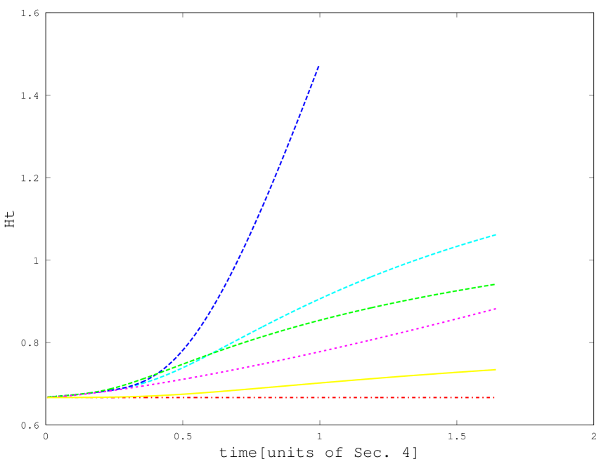
Figure 1: Time evolution of $Ht$

Fig. 1 displays $Ht$ over the time $t$ for various versions of the Hubble rate $H$. The dashed lines in blue (highest), cyan (second) and green (third) correspond to the results of the non-perturbative computations; more precisely, they give $\langle H_{\sharp}\rangle_{\mathrm{pp}}t$ as computed numerically via Eq. (85) for the scenarios 1, 2 and 3, respectively. The fourth line (dotted, magenta) corresponds to the perturbative result (101), the fifth (solid yellow) line to $Ht$ as computed via volume averaging, and the final red dash-dotted line shows the constant EdS value of $H_{\mathrm{EdS}}t=2/3$. The strong deviations from the homogeneous case are a consequence mainly of local anisotropy, by the following mechanism. Consider a region ${\cal R}$ characterized by some specific values of $\theta$ and $\sigma_{ij}$ and pick a frame $\{\mathbf{e}_{1},\mathbf{e}_{2},\mathbf{e}_{3}\}$ in which $\sigma_{ij}$ is diagonal. Assume, without loss of generality, that $\sigma_{11}>\sigma_{22}$ and that originally ${\cal R}$ had the same diameters along the corresponding directions $\mathbf{e}_{1}$, $\mathbf{e}_{2}$. Even though the overall volume expansion of ${\cal R}$ is determined by $\theta$, it will expand faster along $\mathbf{e}_{1}$ and more slowly along $\mathbf{e}_{2}$, so that after a while ${\cal R}$ will have a larger extension in the $\mathbf{e}_{1}$-direction than in the $\mathbf{e}_{2}$-direction. A photon traversing ${\cal R}$ along $\mathbf{e}_{1}$ will not only experience a stronger redshift per unit of time spent in ${\cal R}$ than one moving along $\mathbf{e}_{2}$, but it will also spend more time in ${\cal R}$. The corresponding weighting that favors directions with stronger expansion results in the effect that on average a photon traversing ${\cal R}$ experiences a higher redshift than the volume expansion of ${\cal R}$ would suggest.

Figure 2: Time evolution of $i\sqrt{\bar{g}}$

In Fig. 2 the time evolution of $i\sqrt{\bar{g}}$ is displayed for our three non-perturbative scenarios; to be precise, $\langle i\rangle_{\mathrm{pp}}\langle\sqrt{\bar{g}}\rangle_{\mathrm{mw}}$, i.e. the mass-weighted average of the right-hand side of Eq. (90) is shown. The sharply dropping blue line corresponds to the first scenario, the curved cyan line to the second one, and the mildly dropping green line to the third one. These results are contrasted with the perturbative result $i\sqrt{\bar{g}}\equiv 5/27$ and the EdS value of $i\sqrt{\bar{g}}\equiv 0$ as represented by the two horizontal lines (in dotted magenta and dash-dotted red, respectively). Here the differences between the perturbative and non-perturbative results are not only enormous in magnitude but also change the direction of the effect. Once again the main contributions come from terms involving indicators of local anisotropy such as $\sigma_{ij}$ and $r_{ij}$, as the form of the defining equation (50) suggests.

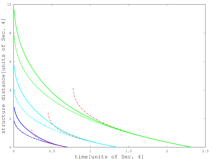
Figure 3: Structure distance over time

Fig. 3 differs from the previous ones by relying not only on $t_{e}=t$ but also on $t_{o}$, the present age of the universe expressed in the dimensionless units of Sec. 4. Here and elsewhere our choice was simply to take $t_{o}$ as the time at which $H_{\sharp}t=1$ (remember that $H_{\sharp}(t_{o})=H_{\mathrm{inf}}(t_{o})$). This is suggested by the fact that it seems to be a very good approximation in the case of the $\Lambda$CDM model and also close to lower bounds coming from ages of globular clusters; in a more general analysis one should probably also allow for values of $H_{o}t_{o}$ somewhat above 1. For our first scenario we find $t_{o}\approx 0.7$ in this way. The three lines ending at that value show various versions of the structure distance as functions of $t=t_{e}\in[0,t_{o}]$: the solid blue line shows $d_{S}$ itself, the dashed blue line below corresponds to $d_{S\sharp}$, and the dash-dotted red line that “starts late” corresponds to an EdS universe with the same value of $H_{o}$, which would have had a shorter lifetime up to now. The other two triplets of lines correspond in an analogous way to the second scenario, where $t_{o}\approx 1.35$, and to the third one with $t_{o}\approx 2.3$.

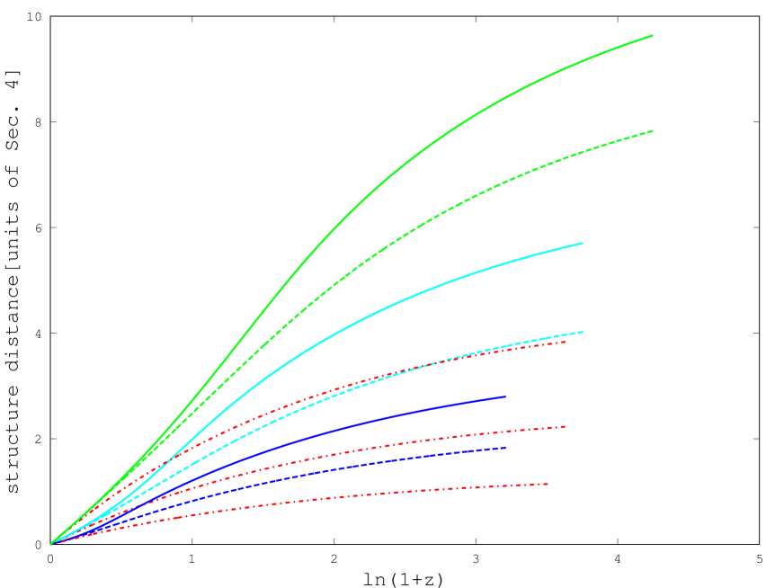
Figure 4: Structure distance over $\ln(1+z)$

For producing Fig. 4, a plot of various versions of the structure distance over $\ln(1+z)$, the result of Eq. (85) (as shown in Fig. 1) was integrated to get $\ln(1+z)$ as a function of $t$, and combined with the values for the structure distance as displayed in Fig. 3. Each scenario is represented by a triplet of lines starting with the same slope which is lowest for the first and highest for the third scenario; the colour and linestyle coding are the same as before. This plot shows that $d_{S}^{\mathrm{(EdS)}}<d_{S\sharp}<d_{S}$, with differences of roughly the same size; i.e. the effect of a proper treatment of the second coefficient $-[\ln(1+z)]\dot{\,}$ in Eq. (16) is of the same order of magnitude as that of a proper treatment of the third coefficient, the quantity $i$.

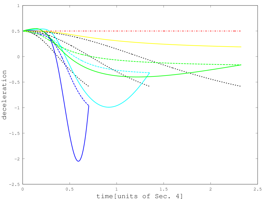
Figure 5: Deceleration over time

Fig. 5 displays various versions of the deceleration parameter over the time $t$. The colour coding is the same as in the previous plots. The dashed lines give $q_{\sharp}$ and the solid blue, cyan and green lines represent $q_{\mathrm{inf}}$; in each case the lines end at our choice for $t_{o}$. The black dotted lines correspond to deceleration in the standard $\Lambda$CDM scenario with $\Omega_{\Lambda}=0.72$, with $t_{o}$ identified with the present time. Again the straight red dash-dotted line represents the EdS scenario, where $q\equiv 1/2$, and the yellow line which shows only a slight downward slope displays the values that one gets via volume averaging. Once again we see that the photon path prescription leads to strongly different results, with effects of roughly the same order coming from the more precise treatments of the two non-trivial coefficients in Eq. (16). While all the results presented so far refer to times and distances in terms of the mathematically convenient but observationally meaningless units of Sec. 4, the following plot uses standard units of years and parsecs.

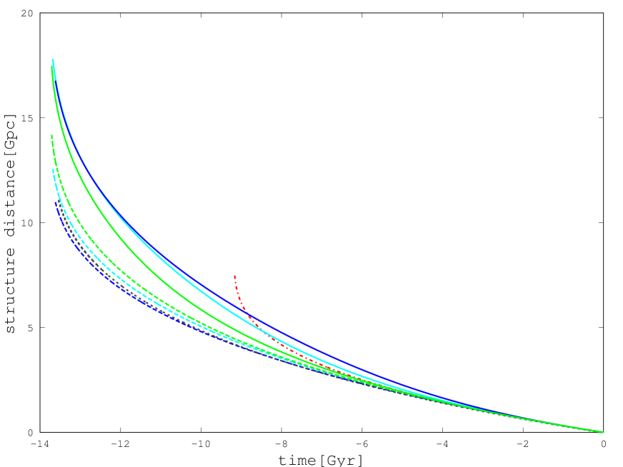
Figure 6: Structure distance over time

Fig. 6 is identical to Fig. 3 except for the normalization and the inclusion of a reference $\Lambda$CDM curve (again as a black dotted line). This figure shows that, with the correct scaling, the predictions of the three different scenarios actually differ less than it appeared originally. Somewhat surprisingly, $d_{S\sharp}$ is closer to the $\Lambda$CDM values than $d_{S}$ here; in particular our results for $d_{S}$ overestimate the distances for early emission times. We can make this discrepancy quite precise by computing the distance to the last scattering surface from which the cosmic microwave background stems (see also Ref. [29]). This is not completely straightforward because the stepwidth of our programs is not fine enough for handling the time $t_{\mathrm{ls}}$ of last scattering that corresponds to $z=1090$. We have circumvented this obstacle by using a combination of our programs and linear perturbation theory to find $t_{\mathrm{ls}}$, noting that the solution of Eq. (16) near $t=0$ takes the form $d_{S}(t)=d_{S}(0)+d_{S}^{(1)}t^{1/3}+{\cal O}(t^{2/3})$, checking that the numerical results for small $t$ are very well fitted by the first two terms, and using them to get $d_{S}(t_{\mathrm{ls}})$. Upon doing this and converting the result to standard units, we found $d_{S}(t_{\mathrm{ls}})\approx 20.7/20.9/19.8~{}\mathrm{Gpc}$ for scenarios 1/2/3, respectively. These numbers overestimate $d_{S}$ by almost 50% compared to Planck results [30] of $13.9~{}\mathrm{Gpc}$ (see their Table 2 and use $d_{S}=r_{*}/\theta_{*}[\mathrm{Mpc}]$), which is the largest discrepancy from standard values that we found in the present work. There are two possible explanations. On the one hand, we have omitted the term $(1+z)^{-2}|{\sigma_{\mathrm{opt}}}|^{2}$ (related to Weyl focusing) in Eq. (50); cf. the discussion after Eq. (85). Inclusion of this term would make the shape of the function $d_{S}(z)$ flatter and therefore more similar to the $\Lambda$CDM reference curve. On the other hand it is not clear whether the angular distance as inferred from the Planck results really should be exactly the same one as that computed via the Sachs equations. The Planck results refer to finite physical distances at $t=t_{\mathrm{ls}}$, whereas the Sachs equations refer to the intersection of the observer’s backward light cone with that timeslice. In the homogeneous case this intersection will be perfectly spherical, but in a realistic inhomogeneous universe it might be somewhat crumpled (more like the surface of an orange), and the distance that corresponds to a total length along that surface (which is what the Sachs equations compute) will be somewhat larger.

Figure 7: Distance (normalized to EdS values) over $z$

Fig. 7 displays, like Fig. 4, distance over redshift, the changes being the normalization of the distance to EdS values, the narrower range of $z$-values, the use of $z$ instead of $\ln(1+z)$, and the inclusion of the $\Lambda$CDM scenario and supernova data. Again the red dash-dotted line corresponds to an EdS universe, the black dotted one to a $\Lambda$CDM universe with $\Omega_{\Lambda}=0.72$, the solid lines to the observed structure distances $d_{S}$ for our three scenarios, and the dashed lines to the values of $d_{S\sharp}$. The black crosses mark the 551 supernovae from the Union2.1 compilation [31] that have $z<1$, as taken from the Supernova Cosmology project website [32]. Both the second and the third scenario perform much better than the EdS case; actually the $\Lambda$CDM curve lies between the second and third scenario for most of the redshift values shown in the plot, and the second one somewhat overestimates the deviation from EdS. The first scenario, in which collapsed regions are included with the values for $[\ln(1+z)]\dot{\,}$ and $i$ that they had in the last moment of collapse, overestimates these deviations even more strongly. This suggests that our model would be improved by introducing a smooth slowing of the collapse (as it happens in reality), with a corresponding smooth transition of $[\ln(1+z)]\dot{\,}$ and $i$ to zero. The fact that even our third scenario, in which we have suppressed the effects from contracting regions, deviates strongly (and in the right direction) from the EdS case demonstrates that such an improvement could not obliterate the total effect of our treatment of inhomogeneities. What have we seen up to now? Considering a universe with $\Lambda=0$ and with distributions of geometric quantities that follow directly from initial conditions based on a Gaussian distribution, and with photons that obey the Sachs optical equations, we have shown that the following facts hold: there is a time $t_{o}$ such that an observer at that time sees a redshift-distance relation remarkably similar to that predicted by the standard $\Lambda$CDM scenario, and if the observer analyses the data without taking into account the inhomogeneities, he will infer a Hubble rate $H_{\mathrm{inf}}$ such that $H_{\mathrm{inf}}t_{o}=1$ and a deceleration parameter $q_{\mathrm{inf}}\approx-0.5$. We have already considered the time $t_{\mathrm{ls}}$ of last scattering in our discussion of Fig. 6. We can make a further, less ambiguous, statement on that era in the following manner. In our most realistic scenario (the second one), $t_{\mathrm{ls}}\approx 5.3\times 10^{-5}$ in the dimensionless units of Sec. 4 (with $t=0$ the instant at which the singularity would have occurred in a purely matter dominated universe). At this time linear perturbation theory is still perfectly valid so that we can compute density perturbations at last scattering with the help of formulas (71) and (70):

$$\left({\Delta\rho\over\rho}\right)_{\mathrm{ls}}=\left({\Delta(a^{-3})\over a^{-3}}\right)_{\mathrm{ls}}={1\over 2}t_{\mathrm{ls}}^{2\over 3}\,\Delta S={1\over 2}\times(5.3\times 10^{-5})^{2\over 3}\times\sqrt{5}\approx 1.6\times 10^{-3}.$$ (108)

These are the density perturbations for the total matter, which are dominated by the ones for dark matter. According to Eq. (2.6.30) of Ref. [21], the density perturbations of baryonic matter satisfy $\Delta\rho_{B}/\rho_{B}=3\Delta T/T$, where $T$ is temperature; using the commonly cited value of $10^{-5}$ for the relative temperature fluctuations in the CMB we find that the total density perturbations are roughly 50 times as large as those for the baryonic matter. This fits very well with the fact that dark matter decouples from photons (hence clumps gravitionally) earlier than baryons. Similar values for the ratios of the baryonic versus total density perturbations are required for structure formation; see e.g. Fig. 1 of Ref. [28]. We can turn this argument around: from the density perturbations we see that the time of last scattering cannot have occurred significantly before the time $t_{\mathrm{ls}}\approx 5.3\times 10^{-5}$ that corresponds to $t_{o}\approx 1.35$. But then it is clear that the inhomogeneities will have a significant impact on inferred Hubble and deceleration rates, so that the assumption that a homogeneous universe (with or without a cosmological constant) give correct predictions necessarily breaks down. Conversely, since we do not require a non-zero $\Lambda$ to account for present observations the simplest assumption is to take $\Lambda=0$.

8 Discussion and outlook

Let us start our discussion with a brief reiteration of our assumptions and conclusions. Considering a universe that

• is matter dominated and obeys the Einstein equations,

• in its early stages was very close to being spatially flat and homogeneous, with only Gaussian perturbations, and

• has vanishing cosmological constant, $\Lambda=0$,

we found that there is a time $t_{o}$ such that observervations made at that time and interpreted with formulas appropriate to the homogeneous case, would suggest

• an inferred Hubble rate $H_{\mathrm{inf}}$ such that $H_{\mathrm{inf}}t_{o}\approx 1$,

• an inferred deceleration parameter of $q_{\mathrm{inf}}\approx-0.5$, and

• density perturbations at a redshift of 1090 that fit well with values required at last scattering to lead to structure formation.

In other words, an observer at time $t_{o}$ in such a universe sees essentially what present day cosmologists see, even though $\Lambda$ vanishes. This is the consequence of a model that has only one parameter (the overall scale) which can be adjusted. Once this parameter has been fixed by any of the three quantities that were just mentioned (and thus $t_{o}$ identified with the present age of the universe), the prediction for either of the other two provides a highly nontrivial test. Our methods have performed very well on both of them. In order to arrive at these results it is essential to consider the effects of inhomogeneities on light propagation (not just on the evolution of volumes), and to use a formalism that transcends perturbation theory. The main steps involve the derivation of the differential equation (16) for the structure distance $d_{S}=(1+z)d_{A}$, and the computation of the two non-trivial coefficients $H_{\sharp}=-[\ln(1+z)]\dot{\,}$ and $i$ that occur in this equation. In the spatially flat homogeneous case $H_{\sharp}$ is just the usual Hubble rate and $i=0$; otherwise each of these coefficients contributes significantly, with effects of roughly the same magnitude, to the deviations in the values of $d_{S}$, $H_{\mathrm{inf}}$ and $q_{\mathrm{inf}}$. The main source of discrepancies from FLRW universes is the local anisotropy, as encoded in the dust shear $\sigma_{ij}$ and the traceless part $r_{ij}$ of the Ricci tensor, and not so much the inhomogeneity which manifests itself by variations of the expansion rate $\theta$ and the spatial Ricci scalar $R$. While Eq. (16) is valid in an arbitrary geometry in which photons follow light-like geodesics, the subsequent computations required a number of approximations:

• The matter was modeled as irrotational dust. While this is an excellent approximation during expansion, it would not permit stable structures such as galaxies and clusters as the results of collapse. Our way of treating this problem, by simply assuming that collapse holds at half the maximum size (or ignoring collapsing regions altogether), is certainly somewhat ambiguous. In particular, the differences between the three variants that we chose show that the results do depend on such details; at the same time our third scenario demonstrates that deviations from the homogeneous case do not stem exclusively from collapse. As we argued in the discussion of Fig. 7, a smoother transition to the virialized state in our framework would probably lead to even better agreement with observations.

• We have replaced statistical quantities by their expectation values in order to arrive at a description in which distance can be seen as a function of redshift, as in homogeneous models (cf. the first paragraph of Sec. 5). From the set of supernova data it is clear that this is a gross oversimplification.

• We assumed a distribution of photon paths in $\mathbf{x}$–space (the space in which our matter is at rest, which starts out as being almost perfectly euclidean) that was the same as if the photons moved along straight lines in that space.

• While exact evolution equations were used for the local scale factor $a$, the shear $\sigma_{ij}$ and the Ricci scalar $R$, the evolution of the traceless part $r_{ij}$ of the Ricci tensor was simplified by ignoring the right-hand side of Eq. (60).

• In our analysis of expressions that arise upon taking photon path averages, we have neglected terms of quadratic or higher order in $\gamma_{ij}$ (a scaled version of the traceless part of the metric $g_{ij}$).

• For reasons that we discussed after Eq. (85) we ignored Weyl focusing, i.e. the contribution of the optical shear $\sigma_{\mathrm{opt}}$.

• For the numerical treatment the time axis and the probability distribution for the background parameters were discretized. The resulting errors are, however, much smaller than those coming from the other approximations.

Unfortunately the second and third item are not as harmless as they originally seemed. Upon replacing $i$ and $H_{\sharp}$ by their expectation values, we have introduced errors $\Delta i$ and $\Delta H_{\sharp}$ which have vanishing expectation values and are of first order. These lead to errors $\Delta d$ and $\Delta\ln(1+z)$ of the same type. The transition from $d(t)$ and $\ln(1+z)(t)$ to $d(z)$ then generates products of errors which are of second order and nonvanishing expectation value. The approximation introduced in the second paragraph of Sec. 5 probably leads to similar problems, whereas our computations in Sec. 6 respect the essential terms at second order perturbation theory. A general $n^{\mathrm{th}}$ order term is an $n$-fold product of $C$ (or, equivalently, the Newtonian potential $\Phi$) or its derivatives, in such a way that typically the $n^{\mathrm{th}}$ order term has a total of up to $2(n-1)$ spatial derivatives more that the first order term (see Ref. [26] for a detailed discussion). While $C$ itself is small, $\partial^{2}C$ can be large; for example, density perturbations are of this type. In particular, among the terms contributing to the redshift-distance relation at second order, the largest ones that we find are proportional to $\langle(\partial^{2}C)^{2}\rangle$. However, according to the two independent groups that have performed complete computations up to second order [10, 12, 17, 18], terms of that type cancel out completely and subleading terms give corrections of an order of magnitude of only around $10^{-4}$. This can be explained in the following way. In our approach, using the synchronous gauge, the whole setup relies on expressing quantities in terms of the entries (or eigenvalues) of the matrix $S_{ij}=\partial_{i}\partial_{j}C$; to be precise, the $n^{\mathrm{th}}$ order contribution to any of the quantities $a$, $\hat{\sigma}$, $\hat{R}$ and $\hat{r}$ is homogeneous of degree $n$ in $S$. Terms of this type also produce the dominant contribution to the deviation of the metric from the FLRW case. But terms of (schematically) type $\partial^{2n}C^{n}$ in $g_{ij}$ give rise to terms of type $\partial^{2n+2}C^{n}$ in the curvature, which must all cancel. This means that the part of the spatial metric consisting of the highest derivatives is flat, implying that it is possible to reparameterize the spatial slices in such a way that the metric no longer contains the $\partial^{2n}C^{n}$ terms. Hence any approximation in the synchronous gauge that does not respect the precise structure of the $\partial^{2n}C^{n}$ terms introduces errors that are potentially larger than the physical effects from the inhomogeneities. Since our approach suffers from this problem, it does not provide a conclusive argument that the standard $\Lambda$CDM picture require modification. Nevertheless it is intriguing how well it appears to perform – after all, one would expect mere errors to result in random nonsense rather than something that closely resembles observations. Besides, standard perturbation theory cannot be trusted either: higher order terms are not smaller than first order terms [26], and the real universe features shell crossings and vorticity, which do not occur in a purely perturbative modelling of an irrotational dust universe, but whose effects are taken into account by the approach to virialization in the present framework. Acknowledgements: It is a pleasure to thank Anton Rebhan and Dominik Schwarz for helpful discussions, and Phil Bull for email correspondence. While a lengthy refereeing process led to some clarifications, the arguments in the last few paragraphs that shed doubt on the approach were developed by myself during a stay at Bielefeld university, for whose hospitality I am very grateful.

References

- [1]
- [2]
- [3] D. J. Schwarz, astro-ph/0209584.
- [4] R. Durrer, Phil. Trans. Roy. Soc. Lond. A 369, 5102 (2011) [J. Cosmol. 15, 6065 (2011)] [arXiv:1103.5331 [astro-ph.CO]].
- [5] T. Mattsson, Gen. Rel. Grav. 42, 567 (2010) [arXiv:0711.4264 [astro-ph]].
- [6] S. Rasanen, JCAP 0902, 011 (2009) [arXiv:0812.2872 [astro-ph]].
- [7] C. Clarkson, G. F. R. Ellis, A. Faltenbacher, R. Maartens, O. Umeh and J. P. Uzan, Mon. Not. Roy. Astron. Soc. 426, 1121 (2012) [arXiv:1109.2484 [astro-ph.CO]].
- [8] P. Bull and T. Clifton, Phys. Rev. D 85, 103512 (2012) [arXiv:1203.4479 [astro-ph.CO]].
- [9] K. Bolejko and P. G. Ferreira, JCAP 1205, 003 (2012) [arXiv:1204.0909 [astro-ph.CO]].
- [10] O. Umeh, C. Clarkson and R. Maartens, Class. Quantum Grav. 31, 202001 (2014) [arXiv:1207.2109 [astro-ph.CO]].
- [11] I. Ben-Dayan, R. Durrer, G. Marozzi and D. J. Schwarz, Phys. Rev. Lett. 112, 221301 (2014) [arXiv:1401.7973 [astro-ph.CO]].
- [12] O. Umeh, C. Clarkson and R. Maartens, Class. Quant. Grav. 31, 205001 (2014) [arXiv:1402.1933 [astro-ph.CO]].
- [13] S. Bagheri and D. J. Schwarz, JCAP 1410, no. 10, 073 (2014) [arXiv:1404.2185 [astro-ph.CO]].
- [14] R. K. Sachs, Proc. Roy. Soc. Lond. A 264, 309 (1961).
- [15] C. C. Dyer and R. C. Roeder, Astrophys. J. 180, L31 (1973).
- [16] I. Ben-Dayan, M. Gasperini, G. Marozzi, F. Nugier and G. Veneziano, JCAP 1204, 036 (2012) [arXiv:1202.1247 [astro-ph.CO]].
- [17] I. Ben-Dayan, M. Gasperini, G. Marozzi, F. Nugier and G. Veneziano, Phys. Rev. Lett. 110, no. 2, 021301 (2013) [arXiv:1207.1286 [astro-ph.CO]].
- [18] I. Ben-Dayan, M. Gasperini, G. Marozzi, F. Nugier and G. Veneziano, JCAP 1306, 002 (2013) [arXiv:1302.0740 [astro-ph.CO]].
- [19] G. Fanizza, M. Gasperini, G. Marozzi and G. Veneziano, arXiv:1506.02003 [astro-ph.CO].
- [20] M. Gasperini, G. Marozzi, F. Nugier and G. Veneziano, JCAP 1107, 008 (2011) [arXiv:1104.1167 [astro-ph.CO]].
- [21] S. Weinberg, “Cosmology,” Oxford Univ. Pr. (2008).
- [22] H. Skarke, Phys. Rev. D 90, no. 6, 063523 (2014) [arXiv:1407.6602 [astro-ph.CO]].
- [23] I. M. H. Etherington, Phil. Mag. 15, 761 (1933), reprinted in Gen. Rel. Grav. 39, 1055 (2007).
- [24] N. Straumann, “General Relativity,” Second Edition, Springer (2013).
- [25] H. Skarke, Phys. Rev. D 89, no. 4, 043506 (2014) [arXiv:1310.1028 [astro-ph.CO]].
- [26] C. Clarkson and O. Umeh, Class. Quant. Grav. 28, 164010 (2011) doi:10.1088/0264-9381/28/16/164010 [arXiv:1105.1886 [astro-ph.CO]].
- [27] Octave community, GNU Octave 3.6.2, www.gnu.org/software/octave/.
- [28] S. Naoz and R. Barkana, Mon. Not. Roy. Astron. Soc. 362, 1047 (2005) [astro-ph/0503196].
- [29] C. Clarkson, O. Umeh, R. Maartens and R. Durrer, JCAP 1411, no. 11, 036 (2014) doi:10.1088/1475-7516/2014/11/036 [arXiv:1405.7860 [astro-ph.CO]].
- [30] P. A. R. Ade et al. [Planck Collaboration], Astron. Astrophys. 571, A16 (2014) doi:10.1051/0004-6361/201321591 [arXiv:1303.5076 [astro-ph.CO]].
- [31] N. Suzuki et al., Astrophys. J. 746, 85 (2012) doi:10.1088/0004-637X/746/1/85 [arXiv:1105.3470 [astro-ph.CO]].
- [32] Supernova Cosmology project, http://supernova.lbl.gov/union/.