Graph Homology and Stability of Coupled Oscillator Networks

Abstract

There are a number of models of coupled oscillator networks where the question of the stability of fixed points reduces to calculating the index of a graph Laplacian. Some examples of such models include the Kuramoto and Kuramoto–Sakaguchi equations as well as the swing equations, which govern the behavior of generators coupled in an electrical network. We show that the index calculation can be related to a dual calculation which is done on the first homology group of the graph, rather than the vertex space. We also show that this representation is computationally attractive for relatively sparse graphs, where the dimension of the first homology group is low, as is true in many applications. We also give explicit formulae for the dimension of the unstable manifold to a phase-locked solution for graphs containing one or two loops. As an application, we present some novel results for the Kuramoto model defined on a ring and compute the longest possible edge length for a stable solution.

1 Introduction

Let $G=(V,E,\Gamma=\{\gamma_{v,w}\}_{v,w\in V})$ be a weighted graph. The Laplacian matrix of $G$ is the $|V|\times|V|$ matrix whose components are

$$(\mathcal{L}_{G})_{vw}=\begin{cases}\gamma_{vw},&v\neq w,\\ -\sum_{u}\gamma_{vu},&v=w.\end{cases}$$

A classical result is that if $\gamma_{vw}\geq 0$, then $\mathcal{L}_{G}$ is negative semidefinite, with the number of zero eigenvalues equal to the number of connected components of the graph $G$. If some of the $\gamma_{vw}$ are negative, then $\mathcal{L}_{G}$ can have positive eigenvalues as well. In [1, 2], the authors consider the problem where some subset of the $\gamma_{vw}$ are negative, and show upper and lower bounds on the number of positive eigenvalues of $\mathcal{L}_{G}$ that depend only on the “sign topology” of the graph, i.e. the pattern of which edges are positive and which are negative, regardless of their weights.

More specifically, the main result of [1] is: assume that the graph is symmetric ($\gamma_{(v,w)}=\gamma_{(w,v)})$, and define $G_{+}$ (resp. $G_{-}$) to be the subgraphs of $G$ containing only edges with positive (resp. negative) weights. Let $|G|$ be the number of components of a graph $G$. If $n_{+}(G)$ is the number of positive eigenvalues of $\mathcal{L}_{G}$, then

$$|G_{+}|-1\leq n_{+}(G)\leq|V|-|G_{-}|.$$ (1.1)

Moreover, one can show that these bounds are saturated, i.e. for any integer in that range, there is some choice of weights that give exactly that many positive eigenvalues. (In fact, one can say much more about the genericity of the sets of weights that give these values, see [2] for more detail.)

It follows from the formula above that if $G$ is a tree, then the number of positive eigenvalues is exactly the number of negatively weighted edges in the graph. To see this, notice that, for a tree, the number of connected components of $G_{+}$ is exactly one plus the number of negative edges: if we start with a tree with only positive edges, every flip of an edge from positive to negative will add another component to the positive subtree. Conversely, since the negative edges cannot form a cycle, the number of connected components of $G_{-}$ is the number of vertices minus the number of negatively weighted edges. In short, if $G$ is a tree, then $n_{+}(G)$ is independent of the weights of the edges, and very easy to compute by inspection.

Now, consider the case where the graph has one cycle and one negative edge. It is easy to see in this case that the upper bound in (1.1) is one, and the lower bound is either zero (if the negative edge lies in the cycle); or one (if the negative edge does not lie in the cycle). In the latter case, the number of positive eigenvalues is again independent of the weights. In the former case, the weight on the edge matters, and it is not hard to imagine that the relative magnitude of the weight on the negative edge compared to the other edges in the cycle determines the stability.

From these examples, it is at least plausible to conjecture that the stability computation is something that can done on a cycle-by-cycle basis. This is further supported by previous work of the authors [1], where it was shown that a certain quotient of $H_{1}(G)$ by a subgroup was important for understanding the spectrum of the graph Laplacian with positive and negative edges.

In fact, this is the result of the current paper. Let us denote the number of cycles by $C=|E|-|V|+1$. Then the main result of this paper is that the computation of the index of $\mathcal{L}_{G}$ is the equivalent to computing the index of a particular $C\times C$ matrix (what we call the “cycle intersection matrix”). If $C\ll|V|$, then this is clearly a much simpler problem; the technique we describe here is most effective for sparse graphs.

1.1 Connection to nonlinearly coupled phase oscillators

As stated above, the problem we consider is a pure linear algebra problem and can be stated as such, but in fact it is inspired and informed by considering its “killer app”, i.e. understanding the dimension of the unstable manifold of a fixed point of a nonlinearly coupled network dynamical system.

Some examples of the kinds of models we are interested in include the Kuramoto problem on a general weighted connected graph $D=\{\delta_{ij}\}$, namely:

$$\frac{d\theta_{i}}{dt}=\omega_{i}+\sum\delta_{ij}\sin(\theta_{j}-\theta_{i}).$$ (1.2)

More generally one can also consider the Kuramoto–Sakaguchi model[3, 4]

$$\frac{d\theta_{i}}{dt}=\omega_{i}+\sum\delta_{ij}\sin(\theta_{j}-\theta_{i}+\alpha),$$ (1.3)

as well as the swing equations, which govern the dynamics of a coupled system of generators and loads[5]

$$M\frac{d^{2}\theta_{i}}{dt^{2}}+D\frac{d\theta_{i}}{dt}=\omega_{i}+\sum\delta_{ij}\sin(\theta_{j}-\theta_{i}).$$ (1.4)

In each of these examples the dimension of the unstable manifold to a fixed point of the equations is given by the number of positive eigenvalues of a graph Laplacian.

The study of the fixed points of these systems, and their stability, has lead to a huge number of papers in the literature [6, 7, 8, 9, 10, 11, 12, 13, 14, 15, 16, 17, 18, 19, 20, 21, 22, 23]. It has been widely observed that the behavior of solutions varies dramatically as the topology of the graph changes: these models are essentially trivial on a tree, but become more complex as the graph becomes denser. This again suggests that the first homology group $H_{1}(D)$, which counts the number of loops in the graph, should be important

To date, most of the analytical work has focused on special graph configurations with a high degree of symmetry. The most-studied case, where the behavior of the model is very well understood, is the case of “all-to-all” coupling, where the underlying graph is the complete graph $K_{n}$, and all of the edge weights $\delta_{ij}$ are equal. In a ground breaking paper [19], Mirollo and Strogatz gave upper and lower bounds (which differed by 1) on the dimension of the unstable manifold to an arbitrary fixed point solution to this model. Dörfler and Bullo [24] gave a sufficient condition for the existence of a stable phase-locked solution, and two of the current authors [25] gave an explicit formula for the dimension of the unstable manifold. Similarly Verwoerd and Mason give a proof of the existence of a critical coupling constant for the cases of the complete[16] and bipartite graphs, and one of the current authors [26] gives some results on the minimizers and saddles for the Kuramoto on cyclic graphs. For general topologies, it was first observed by Ermentrout [27] that if the graph is connected and all of the links are short (the angle differences are less than $\frac{\pi}{2}$) then the fixed point is stable.

We show in this paper that the intuition put forward in the preceeding paragraphs is correct. We show that, rather than computing the number of positive eigenvalues of the Laplacian, an object that acts on the vertex space of the graph, there is a dual calculation that can be posed on the cycle space. This dual problem gives an alternative method for computing the dimension of the unstable manifold to a particular fixed point. This approach is particularly attractive for problems in which the graph is relatively sparse, and the dimension of the cycle space is much smaller than the dimension of the vertex space. We note that there are some very important applications for which this condition is satisfied. One example is the graphs associated with electrical power networks. Such networks are governed by the swing equations (1.4) and these tend to be reasonably sparse. The following data is from Cotilla-Sanchez, Hines, Barrows and Blumsack[28], who calculated the number of edges and vertices for the IEEE 300 model (a standard test power system) as well as the Eastern (EI), Western (WI) and Texas (TI) interconnects, the largest components of the North American electrical network:

Table 1: Sparsities of Various Electrical Networks

Network	Edges $E$	Vertices $N$	Number of Cycles $C=E-N+1$	Sparsity $\frac{C}{N}$
IEEE 300	409	300	110	.37
EI	52075	41228	10848	.26
WI	13734	11432	2303	.2
TI	5532	4513	1020	.23

As can be seen from the data above electrical networks tend to be quite sparse, with the dimension of the cycle space being 20—40% of dimension of the vertex space. For instance if one wanted to understand the stability of a fixed point of the Texas Interconnect, the dual problem presented in this paper would reduce the calculation to the eigenvalues of a $1020\times 1020$ matrix, rather than the $4513\times 4513$ eigenvalue problem determined by a naive stability calculation.

2 Summary of Results

In this section, we define our notation and state the two main theorems of the paper, and give a sense of the main ideas of the proofs. The complete proof of the main results will be deferred to Section 5.

2.1 Definitions

Definition 2.1.

A weighted graph $G$ is the triple $G=(V,E,{\Gamma})$, where $V$ is a set of vertices, $E\subseteq V\times V$ a set of edges, and ${\Gamma}=\{\gamma_{e}\}_{e\in E}$ a set of edge weights. By this definition, the graphs in this paper are always simple (at most one edge between vertices) and undirected.

Definition 2.2.

Let $G=(V,E,{\Gamma})$ be a weighted graph. The Laplacian matrix of $G$ is the $|V|\times|V|$ matrix whose entries are given by

$$(\mathcal{L}_{G})_{v,w}=\begin{cases}\quad\quad\gamma_{(v,w)},&v\neq w,\\ -\sum_{u}\gamma_{(v,u)},&v=w.\end{cases}$$

Since the graph is undirected, the Laplacian matrix is always symmetric and has real spectrum. We denote by $n_{+}(G),n_{0}(G),n_{-}(G)$ the number of positive, zero, and negative eigenvalues of $\mathcal{L}_{G}$, and refer to this triple as the spectral index of $G$. Since, for any $G$, $\mathcal{L}_{G}{\bf 1}={\bf 0}$, $\mathcal{L}_{G}$ has a zero eigenvalue and thus a zero determinant. We define the reduced determinant of $\mathcal{L}_{G}$, $\det_{\mathsf{red}}(\mathcal{L}_{G})$, to be the determinant of the matrix restricted to the space of zero sum vectors, i.e. to the orthogonal complement of ${\bf 1}$ in $\mathbb{R}^{|V|}$. (Note that $\det_{\mathsf{red}}(\mathcal{L}_{G})=0$ iff $\mathcal{L}_{G}$ has a nonsimple eigenvalue at $0$.) We will colloquially refer to a Laplacian as stable if $n_{+}(\mathcal{L}_{G})=0$ and unstable otherwise.

Definition 2.3.

Let $G=G(V,E,{\Gamma})$ be a connected weighted graph. Choose and fix and orientation for each edge (so that each edge has both a head and tail vertex). Define the signed incidence matrix of $G$ as the $|V|\times|E|$ matrix whose entries are given by

$$(B_{G})_{v,e}=\begin{cases}1,&e=(v,*),\\ -1,&e=(*,v),\\ 0,&\mbox{else.}\end{cases}$$

The nullspace of the matrix is called the cycle space. It is a standard result [29] that if $G$ is connected, then the dimension of this nullspace is $C:=|E(G)|-|V(G)|+1$. We call this integer the cycle rank of the graph. Note also that while the definition of $B$ depends on the choice of orientation, the number $C$ does not.

Using the Rank–Nullity Theorem, the above is equivalent to saying that $B_{G}^{\top}$ has nullity one, a fact we also use below. It is also not hard to see that $B_{G}^{\top}{\bf 1}={\bf 0}$, so in fact $\ker(B_{G}^{\top})=\mathop{\rm span}\nolimits({\bf 1})$ whenever $G$ is connected.

We define the tree set $\mathop{\rm Tree}\nolimits(G)$ to be the set of edges of $G$ that are contained in every spanning tree of $G$. The complement of $\mathop{\rm Tree}\nolimits(G)$ is the cycle set $\mathop{\rm Cycle}\nolimits(G)$, consisting of every edge which is included in some cycle in the graph. In terms of the incidence matrix, $e$ is in the cycle set if and only if there is a vector $x\in N(B_{G})$ with $x_{e}\neq 0$.

Definition 2.4.

Let $y_{1},y_{2},\dots,y_{C}$ be a basis for the cycle space. Define the $|E|\times C$ matrix $Y_{G}$ whose columns are given by the $y_{i}$, and $D_{G}$ to be the $|E|\times|E|$ diagonal matrix where the $e$th entry is $\gamma_{e}$. Finally, we define the cycle intersection matrix, or the cycle form

$${\mathcal{Z}}_{G}:=-Y_{G}^{\top}D_{G}^{-1}Y_{G},$$ (2.1)

i.e. the matrix with components

$$({\mathcal{Z}}_{G})_{ij}=-\sum_{e\in E}\gamma_{e}^{-1}{y_{i,e}y_{j,e}}.$$

Note that ${\mathcal{Z}}_{G}$ is always a $C\times C$ matrix. The exact form of ${\mathcal{Z}}_{G}$ will depend on the choice of basis, and we will specify the exact choice of basis in (5.3) below. For now, we simply note that any property that we need for ${\mathcal{Z}}_{G}$ will be independent of this choice.

Lemma 2.5.

Let $G=(V,E,\Gamma)$ be a connected weighted graph. Define $D$ as in Definition 2.4 and $B$ as in Definition 2.3. Then

$$\mathcal{L}_{G}=-B_{G}D_{G}B_{G}^{\top}.$$

Proof.

Let us first assume that $v\neq w$. Then

$$(B_{G}D_{G}B_{G}^{\top})_{v,w}=\sum_{e,e^{\prime}}B_{ve}D_{ee^{\prime}}B^{\top}_{e^{\prime}w}=\sum_{e}B_{ve}B_{we}\gamma_{e}.$$

If $v,w$ are adjacent, then either $e=(v,w)$ or $e=(w,v)$ is an oriented edge. In either case, $B_{ve}B_{we}=-1$. Moreover, if $e$ is an edge not incident on both $v$ and $w$, then $B_{ve}B_{we}=0$, and thus the sum has a single term, and $(B_{G}D_{G}B_{G}^{\top})_{vw}=-\gamma_{e}$. Therefore all of the off-diagonal terms are the same as $-\mathcal{L}_{G}$.

Finally, notice that since $B_{G}^{\top}{\bf 1}={\bf 0}$, we have $B_{G}D_{G}B_{G}^{\top}{\bf 1}={\bf 0}$, and from this it follows that the diagonal terms must be correct as well.

∎

2.2 Theorems

The following are the main results of the paper. The first result gives a formula for the number of positive eigenvalues of the Laplacian in terms of the number of edges with negative edge weights together with the number of positive eigenvalues of the cycle intersection matrix.

Theorem 2.6.

Let $G=(V,E,{\Gamma})$ be a connected, weighted graph and let $\mathcal{L}_{G}$ be its Laplacian matrix. Then the number of positive eigenvalues of the Laplacian is the number of negative edges in the graph minus the number of positive eigenvalues of the cycle intersection matrix, i.e.

$$n_{+}(\mathcal{L}_{G})=\#\{e\in E\,|\,\gamma_{e}<0\}-n_{+}({\mathcal{Z}}_{G}).$$ (2.2)

Recall in the definition of ${\mathcal{Z}}_{G}$ that one makes a choice of basis; however, it follows from Lemma A.3 that the index of ${\mathcal{Z}}_{G}$ is independent of this choice of basis.

In particular, we have the inequality

$$n_{+}(\mathcal{L}_{G})\leq\#\{e\in\mathop{\rm Tree}\nolimits(G)\,|\,\gamma_{e}<0\}.$$

From (2.2), the maximal number of negative edges a graph can have and still have a stable Laplacian is the cycle number $C$. In the case where the Laplacian is stable and there are exactly $C$ negative edges, then there is choice of basis cycles so that there is exactly one negative edge in each cycle in the basis. In other words if there are exactly $C$ negative edges, then the graph with the negative edges removed must be a tree.

Remark 2.7.

The basis for the cycle space can be chosen in the following way: Let $G_{+}$ be the subgraph containing only the edges of $G$ with positive weight. The cycle space of $G_{+}$ forms a subspace $S_{+}$ of the full cycle space of $G$. Similarly let $G_{-}$ be the subgraph containing only negatively weighted edges, and $S_{-}$ the corresponding cycle space. Note that $S_{+}$ and $S_{-}$ are necessarily orthogonal. The basis for the cycle space of the full graph $G$ can be chosen as the union of bases for $S_{+}$ and $S_{-}$ together with a set of “mixed” cycles that cannot be decomposed into a sum of cycles containing only edges of one sign. These mixed cycles are a basis for the quotient of the full group of cycles by the subgroups $S_{\pm}$. In this basis the cycle intersection form can be written in the following partitioned form

$${\mathcal{Z}}_{G}=\left(\begin{array}[]{c|cc}A_{M}&B_{M,+}&B_{M,-}\\ \hline\cr B^{t}_{M,+}&{\mathcal{Z}}_{G_{+}}&0\\ B^{t}_{M,-}&0&{\mathcal{Z}}_{G_{-}}\end{array}\right)$$

where ${\mathcal{Z}}_{G_{+}}$ and ${\mathcal{Z}}_{G_{-}}$ are the cycle intersection forms for the subgraphs $G_{+}$ and $G_{-}$ respectively.

First we note that ${\mathcal{Z}}_{G_{+}}$ is negative definite and ${\mathcal{Z}}_{G_{-}}$ is positive definite, so that $n_{+}({\mathcal{Z}}_{G})$ is at least as large as the dimension of the cycle space of $G_{-}$ and no larger than the dimension of the full cycle space minus the dimension of the cycle space of $G_{+}$. These inequalities are equivalent to the inequalities derived previously by the authors[1].

Secondly we note that the calculation of the index of ${\mathcal{Z}}_{G}$ can be further reduced to a calculation on the space of mixed cycles. In particular by applying the Haynsworth theorem to (2.7) we have that

$$n_{+}({\mathcal{Z}}_{G})=n_{+}(A_{M}-B_{M,+}{\mathcal{Z}}^{-1}_{G_{+}}B^{t}_{M,+}-B_{M,-}{\mathcal{Z}}^{-1}_{G_{-}}B^{t}_{M,-}),$$

and thus the calculation can be reduced to finding the index of a matrix whose size is the number of mixed cycles. However since the above formula requires inversion of the matrices ${\mathcal{Z}}_{G_{\pm}}$ it is not obvious that this is more attractive than working on the full cycle space.

The second theorem is a similar result at the level of determinants rather than the spectral index. This result is not really needed for the applications, but it is proven with similar ideas and provides a nice dual form of the famous matrix tree theorem. This is essentially a weighted version of a theorem proven by Sjogren,[30] though the proof given here is quite different.

Theorem 2.8.

Let $G=(V,E,{\Gamma})$ be connected, and define $\mathcal{L}_{G}$ as above. Let $N_{G}=|V(G)|$, and then

$$\frac{1}{N_{G}}\det_{\mathsf{red}}(\mathcal{L}_{G})=\det({\mathcal{Z}}(G))\times\prod_{e\in E}\gamma_{e}.$$ (2.3)

The quantity $\det({\mathcal{Z}}(G))$ is a homogeneous Laurent polynomial in the edge weights which generates labelled tree complements: each term in the Laurent polynomial represents a set of edges that, when removed from the graph, yield a tree.

Remark 2.9.

There is an obvious connection between the two theorems, but they are not quite equivalent since they address different quantities. For example, Theorem 2.8 seems stronger since it gives an actual number, but it only implies Theorem 2.6 modulo 2.

We defer the proof of these results until a later section, but we will briefly summarize the two main ideas here. The first is that for any $G$, there is a covering tree $T$ (which is a weighted tree), and a graph map $\varphi\colon T\to G$, which is surjective on vertices and bijective on edges. In other words if one identifies certain vertices of the tree $T$ one obtains $G$. The identification of vertices in the graph corresponds at the level of linear algebra to restriction of the Laplacian to a certain subspace, so the Laplacian on any graph can be realized as the restriction of the Laplacian on a tree to an appropriate subspace.

The second idea is to use the Haynsworth theorem[31], which is stated in Lemma A.1. The Haynsworth theorem is a kind of duality result relating the number of positive eigenvalues of a matrix to the number of positive eigenvalues of a $k\times k$ principle minor matrix and the number of positive eigenvalues of the complementary $(n-k)\times(n-k)$ minor of the inverse matrix. In other words, modulo some invertibility assumptions, if $M$ is self-adjoint and $S$ is a subspace of $\mathbb{R}^{N}$, then

$$n_{+}(M)=n_{+}(M|_{S})+n_{+}(M^{-1}|_{S^{\perp}}).$$

Brushing aside some technical points associated with invertibility which will be addressed below, the basic observation is that if we take $M$ to be the Laplacian on the covering tree and $M|_{S}$ to be the Laplacian on the graph $G$, then one can compute that $M^{-1}|_{S^{\perp}}$ is exactly the cycle intersection form $Z_{G}$. For a tree it is easy to see that the number of positive eigenvalues is exactly the number of edges with negative edge-weights, and formula (2.2) follows. There is an analogous identity at the level of determinants, giving (2.3).

3 Linear Examples

3.1 Diamond graph

We consider the simplest graph with cycle rank $C=2$, the diamond graph shown in the left frame of Figure 2, with five edges and four vertices. The Laplace matrix is given by

$$\mathcal{L}_{G}=\left(\begin{array}[]{cccc}-(\gamma_{a}+\gamma_{d}+\gamma_{e})&\gamma_{a}&\gamma_{e}&\gamma_{d}\\ \gamma_{a}&-(\gamma_{a}+\gamma_{b})&\gamma_{b}&0\\ \gamma_{e}&\gamma_{b}&-(\gamma_{b}+\gamma_{c}+\gamma_{e})&\gamma_{c}\\ \gamma_{d}&0&\gamma_{c}&-(\gamma_{c}+\gamma_{d})\end{array}\right)$$

By the matrix-tree theorem, we can obtain the eight labelled spanning trees by considering the $4,4$ cofactor

$$\begin{split}\det\mathcal{L}_{44}(G)&=\left|\begin{array}[]{ccc}-(\gamma_{a}+\gamma_{d}+\gamma_{e})&\gamma_{a}&\gamma_{e}\\ \gamma_{a}&-(\gamma_{a}+\gamma_{b})&\gamma_{b}\\ \gamma_{e}&\gamma_{b}&-(\gamma_{b}+\gamma_{c}+\gamma_{e})\end{array}\right|\\ &=\gamma_{a}\gamma_{b}\gamma_{c}+\gamma_{a}\gamma_{b}\gamma_{d}+\gamma_{a}\gamma_{c}\gamma_{d}+\gamma_{a}\gamma_{c}\gamma_{e}+\gamma_{a}\gamma_{d}\gamma_{e}+\gamma_{b}\gamma_{c}\gamma_{d}+\gamma_{b}\gamma_{c}\gamma_{e}+\gamma_{b}\gamma_{d}\gamma_{e}.\end{split}$$ (3.1)

Let us orient this graph clockwise around the outside, then $1\to 3$. With this orientation, a basis for the cycle space is given by

$$z_{1} =(1,1,0,0,-1)^{t}$$

$$z_{2} =(0,0,1,1,1)^{t}.$$

The cycle intersection matrix $Z_{G}$ is given by

$$Z_{G}=-\left(\begin{array}[]{cc}\dfrac{1}{\gamma_{a}}+\dfrac{1}{\gamma_{b}}+\dfrac{1}{\gamma_{e}}&\dfrac{1}{\gamma_{e}}\\ \\ \dfrac{1}{\gamma_{e}}&\dfrac{1}{\gamma_{c}}+\dfrac{1}{\gamma_{d}}+\dfrac{1}{\gamma_{e}}\end{array}\right).$$

The determinant of this matrix is

$$\det Z_{G}=\dfrac{1}{\gamma_{d}\gamma_{e}}+\dfrac{1}{\gamma_{c}\gamma_{e}}+\dfrac{1}{\gamma_{b}\gamma_{e}}+\dfrac{1}{\gamma_{b}\gamma_{d}}+\dfrac{1}{\gamma_{b}\gamma_{c}}+\dfrac{1}{\gamma_{a}\gamma_{e}}+\dfrac{1}{\gamma_{a}\gamma_{d}}+\dfrac{1}{\gamma_{a}\gamma_{c}}.$$ (3.2)

It is not hard to see that if we multiply (3.2) by $\gamma_{a}\gamma_{b}\gamma_{c}\gamma_{d}\gamma_{e}$, then we obtain the expression in (3.1), verifying Theorem 2.8. The $\det(Z_{G})$ generates labelled tree complements: each term in this Laurent polynomial represents a pair of edges that, when removed from the graph, yield a tree.

Moreover, we can use Theorem 2.6 to compute bounds on the edge weights to determine stability. For ease of notation, we write $\rho_{i}=1/\gamma_{i}$, and

$$w_{1}=\rho_{a}+\rho_{b},\quad w_{2}=\rho_{c}+\rho_{d},\quad w_{12}=\rho_{e}.$$

Then we have

$$Z_{G}=-\left(\begin{array}[]{cc}w_{1}+w_{12}&w_{12}\\ w_{12}&w_{2}+w_{12}\\ \end{array}\right).$$ (3.3)

Let us first consider the case where there is one negative edge. In this case, $Z_{G}$ has either one or zero positive eigenvalues, which is the same as saying that $-Z_{G}$ has one or zero negative eigenvalues. If there is one, then $\mathcal{L}_{G}$ is stable, and if zero, it is unstable.

Note however that $\det Z_{G}<0$ if and only if there is one positive and one negative eigenvalue, which gives the condition

$$(w_{1}+w_{12})(w_{2}+w_{12})-w_{12}^{2}<0,$$

or

$$w_{1}w_{2}+w_{1}w_{12}+w_{2}w_{12}<0.$$

If we assume that $\gamma_{e}<0$, then, solving for $w_{12}$, we obtain the inequality

$$w_{12}<-\frac{w_{1}w_{2}}{w_{1}+w_{2}},$$

or

$$\rho_{e}<-\frac{\rho_{{a}}+\rho_{{b}}+\rho_{{c}}+\rho_{{d}}}{\left(\rho_{{a}}+\rho_{{b}}\right)\left(\rho_{{c}}+\rho_{{d}}\right)}.$$

Notice, for example, that if we assume that $\gamma_{a}\approx 0$, then the $\rho_{a}$ terms dominate, and the condition we obtain for stability is $\gamma_{e}>-(\rho_{c}+\rho_{d})$. Here $\gamma_{b}$ is not relevant, and this makes sense: as $\gamma_{a}\to 0$, the $a,b$ path is almost broken as a loop and thus cannot significantly affect stability, so the condition for stability will be a balance between $e$ and $c,d$.

On the other hand, if one of the edges on the outside is negative (say wlog $\gamma_{a}$), we obtain the inequality

$$w_{1}<\frac{w_{2}w_{12}}{w_{2}w_{12}},$$

or

$$\rho_{{a}}<-\dfrac{\left(\rho_{{c}}+\rho_{{d}}\right)\rho_{{e}}}{\rho_{{c}}+\rho_{{d}}+\rho_{{e}}}-\rho_{{b}}.$$

Note that every $\rho$ on the right-hand side is positive. Note the particular role played by the $\rho_{b}$ term: if we make $\gamma_{b}$ larger, this makes $\rho_{b}$ smaller (in absolute value), making it more difficult for $\rho_{a}$ to cause the instability.

qqqqq

Now, assume the graph has two negative edges and let us try and find conditions for stability. Note that we cannot have both $a,b$ or both $c,d$ negative, since this automatically gives an unstable Laplacian. Therefore we need that at least two of $w_{1},w_{2},w_{12}$ be negative.

The condition that the matrix be stable is that $-Z_{G}$ have two negative eigenvalues, which we can obtain by the condition of having a positive determinant and a negative trace, so

$$w_{1}w_{2}+w_{1}w_{12}+w_{2}w_{12}>0,\quad w_{1}+w_{2}+2w_{12}<0.$$

By symmetry, we only need to consider the case where $w_{1},w_{2}<0$ and where $w_{1},w_{12}<0$. In the former case, there is a negative edge on each of the “outsides” of the graph, and in the latter there is one in the middle.

3.2 One-cycle graphs

Let us now consider the general one-cycle graph and consider the condition for stability. Note that such a graph can have at most one negative edge and still be stable, and, moreover, it cannot be contained in the tree part of the graph, but must be part of the cycle. Therefore we can simplify and consider $R_{N}$, the ring graph on $N$ vertices: this graph has $N$ vertices and $N$ edges, and let us label them so that edge $i$ goes from $i\to i+1$, modulo $N$.

The cycle can be represented by the vector ${\bf 1}$, and thus we have $Z_{G}$ is the $1\times 1$ matrix (i.e. the scalar)

$$Z_{G}=-\sum_{i=1}^{N}\frac{1}{\gamma_{i}}.$$

Thus to obtain a stable Laplacian, we need that $Z_{G}>0$, or

$$\sum_{i=1}^{N}\frac{1}{\gamma_{i}}<0.$$

Assuming that $\gamma_{1}<0$ and the remainder are positive, the condition for stability is

$$\gamma_{1}>\frac{-1}{\displaystyle\sum_{i=2}^{n}\dfrac{1}{\gamma_{i}}}.$$

If all of the positive edges have an equal weight, $\gamma_{i}\equiv\gamma$, then we obtain

$$\gamma_{1}>-\gamma/(n-1).$$

In this case, we see that increasing $\gamma$ helps with stability, whereas increasing the number of edges, all things being equal, hurts stability.

3.3 Two-cycle graphs

We can consider the general two-cycle graph; in fact, we can reuse many of the computations of Section 3.1 above.

As in the previous section, we simplify by assuming that there are no edges in $\mathop{\rm Tree}\nolimits(G)$, i.e. each edge is in one or more cycles. Let us split the edges into three sets $S_{1},S_{2},S_{12}$; the edges in $S_{1}$ are those only in cycle one, those in $S_{2}$ are those only in cycle two, and finally $S_{12}$ are those edges both in cycles one and two. It is clear that we can choose $S_{1},S_{2}$ to be non-empty, but for some graphs, it may then be the case that $S_{12}$ is empty (e.g. a graph with a figure-eight structure). Let us reorder the edges so that when ordered, the sets $S_{1},S_{2},S_{12}$ come in order, and we write $k_{*}=|S_{*}|$. From this we see that we can choose the cycle basis as

$$y_{1}=(1,1,\dots,1,0,\dots,0,1,\dots,1),\quad y_{2}=(0,0,\dots,0,1,\dots,1,1,\dots,1),$$

where the three groups of edges are of length $k_{1},k_{2},k_{12}$. If we then define

$$w_{*}=\sum_{e\in S_{*}}\frac{1}{\gamma_{e}},$$

then we see that the cycle form $Z_{G}$ has the same structure as in (3.3), and the subsequent analysis holds over for this case.

The simplest case is the one where $S_{12}=\emptyset$ and $w_{12}=0$. In this case $Z_{G}$ is diagonal, and the number of positive eigenvalues is exactly the number of negative diagonal entries. For example, let us say that the edge $e$ for which $\gamma_{e}<0$ is in cycle $1$, and thus we need $w_{1}<0$ to have a stable Laplacian. This gives

$$\frac{1}{\gamma_{e}}+\sum_{f\neq e,f\in S_{1}}\frac{1}{\gamma_{f}}<0,$$

or

$$\gamma_{e}>\dfrac{-1}{\sum_{f\neq e,f\in S_{1}}1/{\gamma_{f}}}.$$

This is exactly the condition as in the one-cycle case. Similarly, if the graph has two negative edges, we need both $w_{1},w_{2}<0$ and the conditions on each cycle are decoupled.

In the case where $w_{12}>0$, this gives an analysis similar to that given above. Let us consider the case where there is one negative edge, and it is in both cycles one and two. We again have the condition

$$w_{12}<-\frac{w_{1}w_{2}}{w_{1}+w_{2}}.$$

If, for example, we consider the case where all of the positive edges have the same weight $\gamma$, and the one negative edge has weight $\gamma_{e}<0$, then we have

$$w_{1}=k_{1}/\gamma,\quad w_{2}=k_{2}/\gamma,\quad w_{12}=\frac{k_{12}-1}{\gamma}+\frac{1}{\gamma_{e}}.$$

This simplifies to

$$\frac{1}{\gamma_{e}}<-\frac{1}{\gamma}\left(\frac{k_{1}k_{2}}{k_{1}+k_{2}}+(k_{12}-1)\right).$$ (3.4)

Again, increasing $\gamma$ helps for stability since it makes the condition easier to achieve, but increasing any of $k_{1},k_{2},k_{12}$ makes the condition harder to achieve.

The interpretation of these facts is as follows: clearly, increasing the strength of the positive couplings will make it harder for the negative coupling to destabilize the entire system, and in fact from (3.4) we see that the two weights are effectively linearly related. Moreover, we see that increasing the number of links in either of the cycles makes it easier to destabilize the system, similarly to the case of a single cycle.

4 Nonlinear example — Kuramoto model on a ring

The examples in the previous section studied the stability of linear Laplacians, but we can also use the current results to obtain novel results for nonlinearly coupled oscillators as well — in particular we consider the Kuramoto model.

It has been known for a long time that if we have a fixed point for the Kuramoto model where all of the links are “short”, i.e. the angle difference across a link is less than $\pi/2$ in absolute value, then this gives a stable fixed point, see [27]. We could then pose the question of whether there exist solutions with “long” links that are still stable (this would correspond to having negative off-diagonal terms in the Jacobian). This question was studied numerically in [21]; there the authors considered a large class of random networks and random frequencies, and showed that stable fixed points with long links do exist, but they are exceedingly rare (typically the proportion of stable points found that have long links were less than $1/1000$).

Intuitively, it makes sense that if we make the weight $\delta_{ij}$ on an edge arbitrarily small, then this is possible, but we could then pose the question: can we have a stable long-link solution if the edge weights are all equal? We will show that this answer is affirmative on the ring by a judicious choice of frequencies. In particular, we will answer the following question for the ring topology: given a specific graph topology for the Kuramoto system with equal edge weights, what is the largest possible link for a stable fixed point of the system?

We consider the Kuramoto model as in (1.2), where we assume that the graph is a ring with $n$ vertices and that the edge weights are all equal, and by rescaling we can assume that they are all one, so that $\delta_{i,i+1}=1$ (here and below this sum on the indices is understood modulo $n$). Let $\theta^{*}$ be a fixed point of (1.2). From this we have

$$0=\omega_{i}+\sin(\theta^{*}_{i+1}-\theta^{*}_{i})+\sin(\theta^{*}_{i-1}-\theta^{*}_{i}),$$ (4.1)

and the Jacobian at this point is given by $J$, where

$$J_{i,i\pm 1}=\cos(\theta_{i}^{*}-\theta_{i\pm 1}^{*}),$$

and the diagonal terms are chosen to make it a Laplacian. Then we see from the previous section that it is a stable fixed point if one of the following two conditions are met:

1. For all $i=1,\dots,n$, $\gamma_{i,i+1}:=\cos(\theta_{i}^{\star}-\theta_{i+1}^{\star})>0$;

2. one of the $\gamma_{i,i+1}$ is negative, and

   $$\sum_{i=0}^{n-1}\frac{1}{\gamma_{i,i+1}}=\sum_{i=0}^{n-1}\frac{1}{\cos(\theta_{i}^{\star}-\theta_{i+1}^{\star})}<0.$$ (4.2)

Note that $\cos(\theta)>0$ iff $\left|{\theta}\right|<\pi/2$, and thus the sign of the cosine of the angle difference tells us whether a link is long or short. These conditions can be reinterpreted as saying: the fixed point is stable if all of the links are short, or if there is one long link, then we need the sum of the reciprocals of the edge weights to be negative. The question then remains: is there a configuration $\theta^{\star}$ that is a fixed point of (1.2), has one long link, and satisfies (4.2)?

Let us write $\zeta_{i}=\theta_{i+1}-\theta_{i}$. Note that every term in the right-hand side of (4.1) will be a $\zeta_{i}$, except for the term $\theta_{n-1}-\theta_{0}$ which we can write as $\sum_{i=0}^{n-2}\zeta_{i}$. Then (4.2) becomes

$$\sum_{i=0}^{n-1}\frac{1}{\cos(\zeta_{i})}+\frac{1}{\cos\left(\sum_{i=0}^{n-1}\zeta_{i}\right)}<0.$$ (4.3)

Without loss of generality, let us assume that the longest link is given by the gap $\theta_{n-1}-\theta_{0}$, so that if there is one long link, it is represented by the last term in (4.3).

We can then pose this problem in an alternate form as follows: for any $\eta\in(0,2\pi)$, let us find the maximum of

$$f(\zeta)=\sum_{i=0}^{n-2}\frac{1}{\cos(\zeta_{i})},\mbox{ subject to }g(\zeta)=\sum_{i=0}^{n-2}\zeta_{i}=\eta.$$

Then it is possible to realize a fixed point with largest gap $\eta$ iff

$$\min_{\zeta}f(\zeta)+\frac{1}{\cos\eta}<0.$$

The nice thing we see from the constrained optimization problem is that since the constraint is symmetric up to any permutation of the variables, any internal optimizer must be as well. (We could also use Lagrange multipliers to obtain the same result.) Thus the maximum of $f$ is acheived only when all of the $\zeta_{i}$ are equal, and (4.3) becomes

$$\frac{n-1}{\cos(\zeta)}+\frac{1}{\cos((n-1)\zeta)}<0.$$ (4.4)

Summarizing our conditions, if we assume that $\cos(\zeta)$ is positive, then iff the conditions

$$\cos((n-1)\zeta)>0\mbox{ or }(\cos((n-1)\zeta)<0\mbox{ and }\frac{n-1}{\cos(\zeta)}+\frac{1}{\cos((n-1)\zeta)}<0$$

hold, then we have a stable fixed point for the solution $\theta_{k}^{*}=k\zeta$. Note that both of these conditions can be simplified to require that their product be positive, i.e.

$$h_{n}(\zeta):=(n-1)\frac{\cos(n-1)\zeta}{\cos(\zeta)}+1>0.$$ (4.5)

To exhibit a “long link” solution, we need to show that there is $\zeta^{*}$ with roots of $h_{n}(\zeta^{*})=0$ and $|n\zeta^{*}\pmod{2}\pi|\in(\pi/2,3\pi/2)$. We will show numerically that this is possible for every $n$, see Table 2.

$n$	$n\zeta^{*}/2\pi$
3	0.447
4	0.392
5	0.358
10	0.297
20	0.272
30	0.264
40	0.261
50	0.258

Table 2: Length of longest possible link for a stable solution on the ring with $n$ vertices

Here we have found the first root of $h_{n}(\zeta)$ and compute $n\zeta_{n}$: this is the distance between $\theta_{0}$ and $\theta_{n-1}$ if we choose the solution $\theta_{k}=k\zeta^{*}$. Note that in each case, the length of the link is greater than a quarter turn (note that we are presenting the length divided by $2\pi$, so that a link is “long” iff it is greater than $1/4$), but this distance decreases monotonically to $1/4$ as $n\to\infty$.

Note that in general, $h_{n}(\zeta)$ has multiple roots, so that the first root may not always give the largest link, but we have found empirically that this is so. As such, the numbers in Table 2 represent the longest link possible for a stable fixed point of the Kuramoto system on a ring of size $n$.

We can also compute the values of $\omega_{k}$ that give this solution. For all $k=1,\dots,n-2$, we have $\theta_{k+1}-\theta_{k}=\theta_{k-1}-\theta_{k}=\zeta$, so that $\omega_{k}=0$. However, we also have

$$\omega_{n-1}(\zeta):=-\sin(\theta_{0}-\theta_{n-1})-\sin(\theta_{n-2}-\theta_{n-1})=\sin((n-1)\zeta)+\sin(\zeta),$$

and $\omega_{0}=-\omega_{n-1}$.

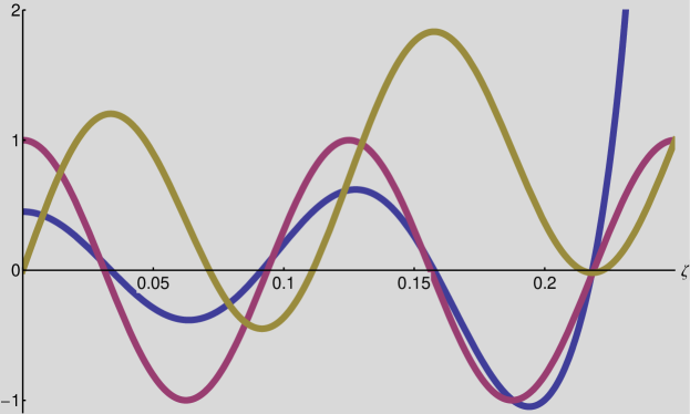
Fig. 1: We plot several of the functions referenced in the text for $n=9$ vertices in the ring: $0.05*h_{9}(\zeta)$ (blue), $\omega_{8}(\zeta)$ (orange), $\cos(8\zeta)$ (purple).

We plot several of the curves for the case of $n=9$ in Figure 1. We have scaled $h_{9}(\zeta)$ so that all the curves are of the same order of magnitude; note that only its sign matters. As shown above, where the blue curve is positive, the solution is stable. The purple curve is the cosine of the length of the $(n-1,0)$ link: since we see that this becomes negative before $h_{9}(\zeta)$ does, there is a stable long link configuration. Finally, note that the zeros of $h_{9}(\zeta)$ correspond to the critical points of $\omega_{8}(\zeta)$ (this can be checked), and thus the $\omega_{8}(\zeta)$ curve can be interpreted as a series of stable and unstable branches: whenever $\omega_{8}(\zeta)$ is increasing in $\zeta$, this corresponds to a stable solutions, and when it is decreasing, this corresponds to a $1$-saddle. As we slide up and down in this graph, this leads to saddle–node bifurcations in the obvious manner. Moreover, note that the $\omega=0$ slice is the one considered in [26] — it was shown there that for $n=9$ there are two nontrivial sinks and two corresponding saddles, and this is recovered here. By decreasing or increasing $\omega_{7}$, we can cause these saddles to collide with either of two sinks.

5 Proof of Theorems

5.1 Proof of Theorem 2.6

5.1.1 Definition of covering tree

Definition 5.1.

Let $G=(V,E,{\Gamma})$ be a connected graph. We define the universal cover of $G$, denoted $U(G)$. If $G$ is a tree, then $U(G)=G$. If $G$ is not a tree, then $U(G)$ is a countably infinite tree defined as follows:

• Choose a root vertex $r\in V(G)$.

• The vertices of $U(G)$ are non-backtracking rooted paths in $G$, i.e. sequences of the form $w=(r,v_{2},v_{3},\dots,v_{n})$ where $(v_{i},v_{i+1})\in E$, and $v_{i-1}\neq v_{i+1}$ for all $i$.

• We say that two vertices $w_{1},w_{2}\in V(U(G))$ are adjacent if one is an extension of the other, i.e.

  $$w_{1}=(r,v_{2},v_{3},\dots,v_{n}),\quad w_{2}=(r,v_{2},v_{3},\dots,v_{n},v_{n+1}),$$

  or vice versa.

• Finally, we define the weight of the edge $(w_{1},w_{2})$ in the example above to be the same as the weight on the edge $(v_{n-1},v_{n})$.

Definition 5.2 (Fundamental domain).

For any graph $G=(V,E,{\Gamma})$, we define $T$, a fundamental domain of the cover of $G$, as follows. First construct the universal cover $U(G)$. Choose $T$ to be any finite connected subtree of $U(G)$ such that each edge of $G$ appears once. Notice that by definition, $G$ and $T$ have the same edge sets, so we will write $E$ for either set. Since there are $|E|$ edges in $T$ and it is a tree, then $|V(T)=|E|+1$. We will also use the notation $N_{G}=|V(G)|$ and $N_{T}=|V(T)|$ throughout.

Remark 5.3.

The universal cover has certain properties:

1. If $G$ is not a tree, then $U(G)$ has countably many vertices. The degree of the node $w=(r,v_{2},\dots,v_{n})$ in $U(G)$ is the same as the degree of $v_{n}$ in $G$. In particular, $U(G)$ is locally finite.

2. The map

   $$\varphi\colon U(G) \to G,$$

   $$(r,v_{2},\dots,v_{n}) \mapsto v_{n}$$

   is a covering map, i.e. it is a map of graphs, it is surjective, and it is an isomorphism in the neighborhood of any vertex.

3. The construction of $T$ is independent (up to isomorphism) of the choice of the root vertex $r$.

4. Finally, it should be noted that we can construct $T$ directly without using the universal cover, see Example 5.5 for an example.

Proposition 5.4.

Let $G=(V,E,{\Gamma})$ be a connected weighted graph, and define $T$ as above. Then the graph map $\varphi\colon T\to G$ given by

$$\varphi((r,v_{2},\dots,v_{n}))=v_{n}$$

is a surjective map. Note that $|V(T)|-|V(G)|=C$, i.e. the difference in the number of vertices of a fundamental domain of the covering tree and the original graph itself is the cycle rank of the graph.

Proof.

Assume that $w_{1},w_{2}\in V(T)$ and $(w_{1},w_{2})\in E(T)$. Since $w_{1},w_{2}$ are adjacent in $U(G)$, we have that

$$w_{1}=(r,v_{1},\dots,v_{k}),\quad w_{2}=(r,v_{1},\dots,v_{k},v_{k+1}),$$

and $(v_{k},v_{k+1})\in E(G)$. Then $\varphi(w_{1})=v_{k}$ and $\varphi(w_{2})=v_{k+1}$ are adjacent in $G$ whenever $w_{1},w_{2}$ are adjacent in $T$. Therefore $\varphi$ is a graph homomorphism. To see that it is surjective, note that every edge of $G$ appears in $T$, and therefore its incident vertices must as well. Finally, note that

$$|V(T)|-|V(G)|=|E|+1-|V(G)|=C.$$

∎

Fig. 2: The diamond graph $G$, and a choice of fundamental domain of its universal cover $T$. Note that $G$ and $T$ have the same edge sets with five edges, and $T$ necessarily has six vertices.

Example 5.5.

Let us consider the diamond graph in Figure 2. If we choose the root vertex as $1$, then $2,3,4$ are neighbors and so we add $12,13,14$ to $T$. Since $\gamma_{b},\gamma_{c}$ have not yet appeared, we add them as in the tree. Of course, this is not the only covering tree we can obtain, even assuming that we choose $1$ as the root; for example, if we remove vertex $143$ and add a vertex $1234$, this would also be a covering tree.

5.1.2 The projections

Definition 5.6.

Let $G$ be a connected graph, and $T$, $\varphi\colon T\to G$ as defined above. We define $X$ to be the $N_{T}\times N_{G}$ matrix whose elements are

$$X_{a,v}=1(\varphi(a)=v).$$

We will also refer to the columns by the vectors $x^{v},v\in V(G)$.

Lemma 5.7.

Let $G=(V,E,{\Gamma})$ be a connected weighted graph, and $T,X$ as in Definitions 5.2, 5.6. Then

$$\mathcal{L}_{G}=X^{\top}\mathcal{L}_{T}X,$$ (5.1)

or

$$(\mathcal{L}_{G})_{v,w}=\left\langle{{x^{v}}},{{\mathcal{L}_{T}x^{w}}}\right\rangle.$$ (5.2)

Proof.

Let us use formula (5.2). Writing this out, we have

$$\left\langle{{x^{v}}},{{\mathcal{L}_{T}x^{w}}}\right\rangle=\sum_{i,j}x^{v}_{i}(\mathcal{L}_{T})_{ij}x^{w}_{j}=\sum_{i,j}(\mathcal{L}_{T})_{ij}1_{\varphi(i)=v}1_{\varphi(j)=w}.$$

If we can show that there exists a unique pair $i,j$ such that $\varphi(i)=v$, $\varphi(j)=w,$ and $(\mathcal{L}_{T})_{ij}=\gamma_{(v,w)}$, then we are done. But notice that since $\varphi(i)=v$, and $\varphi(j)=w$, if $(i,j)\in E(T)$, then the weight on the edge $(i,j)$ must be $\gamma_{(v,w)}$, since $\varphi$ is a graph homomorphism. Moreover, since each edge of $G$ can appear at most once in $T$, this means that there is only one such pair. ∎

Definition 5.8.

The map $\varphi\colon T\to G$ is surjective but in general not injective. For each $v\in V(G)$ with $\left|{\varphi^{-1}(v)}\right|>1$, choose one representative of $\varphi^{-1}(v)$ as the primary representative of this set. Now, for each $w\in\varphi^{-1}(v)$ with $w\neq\mathop{\rm prim}\nolimits(v)$, define the vector $q^{w}\in\mathbb{R}^{N_{T}}$ by

$$q^{w}_{i}=\begin{cases}-1,&i=\mathop{\rm prim}\nolimits(v),\\ 1,&i=w,\\ 0,&else.\end{cases}$$

We define $Q$ as the matrix whose columns are the $q^{w}$.

Lemma 5.9.

Let $S\subseteq\mathbb{R}^{N_{T}}$ be the span of the $x^{v}$ defined in Definition 5.6. Then the vectors $q^{w}$ form a basis for $S^{\perp}$. In particular, $\dim(\mathop{\rm span}\nolimits(q^{w}))=\mathop{\operator@font rank}\nolimits(Q)=c$, the cycle rank of $G$.

Proof.

First we see that each $q^{w}$ is orthogonal to $S$. Consider $x^{v}$ where $v=\varphi(w)$. This vector is equal to $1$ both in the $\mathop{\rm prim}\nolimits(v)$ and $w$ index, and therefore $\left\langle{{q^{w}}},{{x^{v}}}\right\rangle=0$. Moreover, if we consider $x^{v}$ with $v\neq\varphi(w)$, then this vector is equal to zero on these indices, and again $\left\langle{{q^{w}}},{{x^{v}}}\right\rangle=0$. Since $\dim(\mathop{\rm span}\nolimits(S))=\mathop{\operator@font rank}\nolimits(X)=|V(G)|$, so that $\mathop{\operator@font rank}\nolimits(Q)=|E|+1-\dim S=|E|-|V(G)|+1=c$. Finally, note that the $q^{w}$ are clearly independent by construction, so by dimension counting they form a basis for $S^{\perp}$.

∎

Lemma 5.10.

The Laplacian $\mathcal{L}_{T}\colon\mathbb{R}^{N_{T}}\to\mathbb{R}^{N_{T}}$ is not invertible, but has a one-dimensional nullspace given by $\mathop{\rm span}\nolimits({\bf 1})$. In this case, the canonical map

$$\widetilde{\mathcal{L}}_{T}\colon\mathbb{R}^{N_{T}}/\{{\bf 1}\}\to\mathbb{R}^{N_{T}}/\{{\bf 1}\}$$

is invertible. We then have that

$$Q^{\top}(\widetilde{\mathcal{L}}_{T})^{-1}Q={\mathcal{Z}}_{G}.$$

Proof.

In general, for any graph $H$, the incidence matrix $B_{H}$ is map from $\mathbb{R}^{|E(H)|}$ to $\mathbb{R}^{|V(H)|}$. In particular, since $|E(T)|=|E(G)|$ and $|V(T)|=|E(G)|+1$, this means that

$$B_{T}\colon\mathbb{R}^{|E(T)|}\to\mathbb{R}^{|V(T)|}$$

is a map of co-rank one, and as such $B_{T}^{\top}$ is a map with a one-dimensional nullspace, which is $\mathop{\rm span}\nolimits({\bf 1})$. Therefore we can define $\widetilde{B}$ to be the canonical map so that

$$\widetilde{B}\colon\mathbb{R}^{|E(T)|}\to\mathbb{R}^{|E(T)|+1}/\{{\bf 1}\}$$

is invertible: to define this, we first define $\widetilde{B}^{\top}$ to be the induced map on the quotient and then $\widetilde{B}=(\widetilde{B}^{\top})^{\top}$. In particular, note that $\widetilde{B}=B$ on ${\bf 1}^{\perp}$.

For each $w$ such that $q^{w}\neq\mathbf{0}$, consider the unique path in $T$ from $w$ to $\mathop{\rm prim}\nolimits(\varphi(w))$. Let us write this path as

$$w=v_{0}\to v_{1}\to v_{2}\to\dots\to v_{n-1}\to v_{n}=\mathop{\rm prim}\nolimits(\varphi(w)).$$

Define a vector $r^{w}\in\mathbb{R}^{|E(T)|}$ as follows:

$$r^{w}_{e}=\begin{cases}1,&e=(v_{i},v_{i+1}),\exists i,\\ -1,&e=(v_{i+1},v_{i}),\exists i,\\ 0,&\mbox{else.}\end{cases}$$

We first compute that

$$B_{T}r^{w}=q^{w}.$$

To see this, note that $B_{T}r^{w}=0$ on any vertex not in the path, and, moreover, will be zero on any vertex on the interior of the path due to cancellation. We need only consider the endpoints.

First, assume that $w\to v_{1}$ is the chosen orientation for the edge. Then $(B_{T}r^{w})_{w}=((B_{T})_{(w,v_{1})}r_{(w,v_{1})}=1\cdot 1=1$. If, on the other hand, $v_{1}\to w$ is the orientation, then we have $(B_{T}r^{w})_{w}=((B_{T})_{(w,v_{1})}r_{(w,v_{1})}=-1\cdot-1=1$ as well. Similarly, $(B_{T}r^{w})_{\mathop{\rm prim}\nolimits(\varphi(w))}=-1$.

From this, it follows that if we define

$$Y=\widetilde{B}_{T}^{-1}Q,$$ (5.3)

then the columns of $Y$ form a basis for the cycle space of $G$.

By Lemma 2.5, $\mathcal{L}_{T}=-B_{T}DB_{T}^{\top}$, and it is easy to see that similarly, $\widetilde{\mathcal{L}}_{T}=-\widetilde{B}_{T}D\widetilde{B}_{T}^{\top}$. From this we have

$$Q^{\top}(\widetilde{\mathcal{L}}_{T})^{-1}Q=-Q^{\top}\widetilde{B}^{-\top}_{T}D\widetilde{B}_{T}^{-1}Q=-Y^{\top}DY,$$

giving the definition (2.1).

∎

Proof of Theorem 2.6. Recall the definition of $M:=\widetilde{\mathcal{L}}(T)$. From Lemma 5.7 we have that

$$\widetilde{\mathcal{L}}_{G}=X^{\top}\widetilde{\mathcal{L}}_{T}X,$$

and Lemma A.3 gives that

$$n_{+}(\mathcal{L}_{G})=n_{+}(M|_{S}),$$

since the columns of $X$ form a basis for $S$. From Lemma 5.10 we have that

$${\mathcal{Z}}_{G}=Q^{\top}(\widetilde{\mathcal{L}}_{T})^{-1}Q,$$

and Lemma A.3 again gives that

$$n_{+}({\mathcal{Z}}_{G})=n_{+}((M)^{-1}|_{S^{\perp}}),$$

since the columns of $Q$ form a basis for $S^{\perp}$. Using Lemma A.1 gives

$$n_{+}(\mathcal{L}_{G})=n_{+}(\mathcal{L}_{T})-n_{+}({\mathcal{Z}}_{G}).$$

Recall that $T$ is a tree. Using Theorem 2.10 of [1], this implies that the number of positive eigenvalues of $\mathcal{L}_{T}$ are given exactly by the number of negative edges in $E(T)$. Recalling that the edge sets of $G$ and $T$ are the same, we are done.

Finally, to prove the last sentence of the theorem, we again appeal to Theorem 2.10 of [1]. One consequence of this theorem is that for $\mathcal{L}_{G}$ to be stable, $G_{+}$ must be connected. If the number of negative edges in $G$ is the same as the number of cycles, this means that $G_{+}$ is a tree, and thus is a spanning tree of $G$. For each negative edge in $G$, consider the two incident vertices and the unique path in $G_{+}$ connecting them. This plus the addition of the negative edge make a cycle in $G$, and it is clear that each negative edge will be in a different cycle. Using this choice of cycles, we now have exactly one negative edge in each cycle.∎

5.2 Proof of Theorem 2.8

We again start with several lemmas.

Definition 5.11.

Recall $G,T,\varphi\colon T\to G$. For each $v\in V(G)$, if $|\varphi^{-1}(v)|=1$, let $\psi(v)=\varphi^{-1}(v)$; else, $\psi(v)=\mathop{\rm prim}\nolimits(v)$ as defined in Definition 5.8. Then order the vertices of $V(T)$ so that we list all of the vertices in the range of $\psi$ first, and then all of the other vertices in some order. It is easy to see that the range of $\psi$ as $N_{G}$ elements.

We then define the first $N_{G}$ columns of the same way as we did in the definition of $X$, i.e. for $v\in V(G)$, define the $v$th column of $U$, $u^{v}$, by

$$(u^{v})_{a}=\begin{cases}1,&\varphi(a)=v,\\ 0,&\mbox{else},\end{cases}$$

and for columns $i=N_{G}+1,\dots,N_{T}$, define $u^{i}$ to be the standard basis function with a 1 in the $i$th slot. By construction, $U$ is a lower triangular matrix with $1$s on the diagonal, so $\det(U)=1$.

Lemma 5.12.

The $N_{G}\times N_{G}$ upper-left block of $U^{\top}\mathcal{L}_{T}U$ is $\mathcal{L}_{G}$.

Proof.

The proof is more or less the same as Lemma 5.7. Notice that once we have chosen this ordering, the first $N_{G}$ columns of $U$ is the matrix $X$ as defined in Definition 5.6 with the corresponding ordering of vertices. ∎

Lemma 5.13.

Let $H$ be a symmetric matrix with a one-dimensional nullspace, and let $x$ span this nullspace. Then for any $y,z$, we have

$$\det(H+y\otimes z)=\frac{\left\langle{{x}},{{y}}\right\rangle\left\langle{{x}},{{z}}\right\rangle}{\left\langle{{x}},{{x}}\right\rangle}\det_{\mathsf{red}}H.$$

Proof.

Since $H$ is self-adjoint, it has real eigenvalues and a orthonormal eigenbasis. Let us write $\lambda_{1}=0$ with $\lambda_{2},\dots,\lambda_{n}$ not zero, and let $w_{1},\dots,w_{n}$ be the corresponding eigenvectors. Let $W$ be the matrix whose columns are the $w_{i}$; since the eigenvectors form an orthonormal basis, $W^{-1}=W^{\top}$.

Let $M_{1}$ be the diagonal matrix whose diagonal entries are the $\lambda_{i}$, and define $M_{2}=(W^{\top}y)\otimes(W^{\top}z)$, i.e.

$$(M_{2})_{ij}=\left\langle{{w_{i}}},{{y}}\right\rangle\left\langle{{w_{j}}},{{z}}\right\rangle.$$

Notice that $H=WM_{1}W^{\top}$, since this is just its diagonalization, and

$$WM_{2}W^{\top}=W((W^{\top}u)\otimes(W^{\top}w))W^{\top}=WW^{\top}(u\otimes w)WW^{\top}=u\otimes w,$$

where we have used the identity $(Ax)\otimes(By)=A(x\otimes y)B^{\top}$. Thus we have

$$H+u\otimes w=W(M_{1}+M_{2})W^{\top},$$

and since $W$ is unitary this gives

$$\det(H+u\otimes w)=\det(M_{1}+M_{2}).$$

To compute the last term, notice that we can use the multilinearity of the determinant by rows and break up this into $2^{n}$ terms. However, note two things: the matrix $M_{2}$ is rank one and thus has only one linearly independent row, so if we choose more than one row from $M_{2}$, the determinant is zero. Also, the first row of $M_{1}$ is zero, so to obtain a nonzero determinant, we must choose the first row of $M_{2}$. Therefore the only term which gives a nonzero determinant is the one where we choose the first row from $M_{2}$ and all of the other rows from $M_{1}$. Expanding by minors in the first column, the determinant of this matrix is

$$\left\langle{{w_{1}}},{{y}}\right\rangle\left\langle{{w_{1}}},{{z}}\right\rangle\lambda_{2}\times\dots\times\lambda_{n}.$$

Since we chose $\lambda_{1}=0$, this means that $w_{1}$ is the unit vector that spans $\ker(H)$, and also notice that $\det_{\mathsf{red}}H$ is by definition $\lambda_{2}\times\dots\times\lambda_{n}$. Thus we have

$$\det(H+y\otimes z)=\left\langle{{w_{1}}},{{y}}\right\rangle\left\langle{{w_{1}}},{{z}}\right\rangle\det_{\mathsf{red}}H$$

If $x$ is a general vector in $\ker(H)$, then $x$ is a scalar multiple of $w_{1}$ and we have

$$\det(H+y\otimes z)=\frac{\left\langle{{x}},{{y}}\right\rangle\left\langle{{x}},{{z}}\right\rangle}{\left\langle{{x}},{{x}}\right\rangle}\det_{\mathsf{red}}H.$$

∎

Proof of Theorem 2.8. Recall the definition of $U$ in Definition 5.11. Define

$$A=U^{\top}(\mathcal{L}_{T}+\mathbf{1}\otimes\mathbf{1})U=U^{\top}\mathcal{L}_{T}U+U^{\top}\mathbf{1}\otimes U^{\top}\mathbf{1}.$$

If we can establish the following three identities:

$$\det(A) =N_{T}^{2}\prod_{e\in E(G)}\gamma_{e},$$ (5.4)

$$\det(A|_{S}) =\frac{N_{T}^{2}}{N_{G}}\det_{\mathsf{red}}\mathcal{L}_{G},$$ (5.5)

$$\det((A^{-1})|_{S^{\perp}}) =\det({\mathcal{Z}}_{G}),$$ (5.6)

then, using Lemma A.2, we obtain

$$N_{T}^{2}\prod_{e\in E(G)}\gamma_{e}=\frac{\dfrac{N_{T}^{2}}{N_{G}}\det_{\mathsf{red}}\mathcal{L}_{G}}{\det({\mathcal{Z}}_{G})},$$

and this proves the theorem. So it remains to show these three identities.

Identity (5.6) follows directly from Lemma 5.10. To establish (5.4), we note that

$$\det(A)=\det(U^{\top}(\mathcal{L}_{T}+\mathbf{1}\otimes\mathbf{1})U)=\det(\mathcal{L}_{T}+\mathbf{1}\otimes\mathbf{1}),$$

since $\det(U)=1$. By Lemma 5.13, we have

$$\det(\mathcal{L}_{T}+\mathbf{1}\otimes\mathbf{1})=\frac{\left\langle{{\mathbf{1}}},{{\mathbf{1}}}\right\rangle\left\langle{{\mathbf{1}}},{{\mathbf{1}}}\right\rangle}{\left\langle{{\mathbf{1}}},{{\mathbf{1}}}\right\rangle}\det_{\mathsf{red}}\mathcal{L}_{T}=N_{T}\det_{\mathsf{red}}\mathcal{L}_{T},$$

and since there is only one spanning tree of $T$, by the Matrix Tree Theorem,

$$\det_{\mathsf{red}}\mathcal{L}_{T}=N_{T}\prod_{e\in E(G)}\gamma_{e}.$$

To establish (5.5), note that if we use the basis for $\mathbb{R}^{N_{T}}$ made from the columns of $U$, then $A|_{S}$ is just the upper left $N_{G}\times N_{G}$ block of $A$, which is itself the upper left block of $U^{\top}\mathcal{L}_{T}U+U^{\top}\mathbf{1}\otimes U^{\top}\mathbf{1}$. By Lemma 5.12, the upper left block of the first term is just $\mathcal{L}_{G}$, and the upper left block of the second term can be written as

$$\widetilde{U}^{\top}\mathbf{1}\otimes\widetilde{U}^{\top}\mathbf{1},$$

where $\widetilde{(}U)$ is just the first $N_{G}$ columns of $U$. In particular, the $v$th row of $\widetilde{U}^{\top}\mathbf{1}$ is a zero-one vector with as many ones as vertices in $\varphi^{-1}(v)$, and therefore $u:=\widetilde{U}^{\top}\mathbf{1}$ is a column vector of height $N_{G}$ whose $v$th entry is $\left|{\varphi^{-1}(v)}\right|$.

Putting this together, and again using Lemma 5.13 gives

$$\det(A|_{S})=\det(\mathcal{L}_{G}+u\otimes u)=\frac{\left\langle{{u}},{{\mathbf{1}}}\right\rangle\left\langle{{u}},{{\mathbf{1}}}\right\rangle}{\left\langle{{\mathbf{1}}},{{\mathbf{1}}}\right\rangle}\det_{\mathsf{red}}\mathcal{L}_{G}=\frac{\left(\sum_{v\in V(G)}\varphi^{-1}(v)\right)^{2}}{N_{G}}\det_{\mathsf{red}}\mathcal{L}_{G}=\frac{N_{T}^{2}}{N_{G}}\det_{\mathsf{red}}\mathcal{L}_{G}.$$

∎

Appendix A Classical lemmae

This follows from the following duality formula for the number of negative eigenvalues (or more generally the inertia) of a matrix. This result seems to have been frequently rediscovered but the first instance we have found in the literature is due to Haynsworth [31]. This result has been used frequently in the nonlinear waves literature, in the context of the stability of traveling wave solutions.

Lemma A.1 (Haynsworth).

Suppose that $M$ is a non-singular $N\times N$ Hermitian matrix. Let $S$ a subspace of subspace of $\mathbb{R}^{N}$, $S^{\perp}$ the orthogonal subspace, $P_{S}$ the orthogonal projection onto $S$, and $M|_{S}=P_{S}MP_{S}$ the restriction of $M$ to $S$. If $M|_{S}$ is non-singular, then

$$n_{+}(M)=n_{+}(M|_{S})+n_{+}((M^{-1})|_{S^{\perp}})$$

Note that, in her original paper, Haynsworth states this theorem slightly differently in terms of the Schur complement of the matrix, but it is obviously equivalent.

Lemma A.2.

Suppose that $M$ is a non-singular $N\times N$ Hermitian matrix. Let $S$ a subspace of subspace of $\mathbb{R}^{N}$, $S^{\perp}$ the orthogonal subspace, $P_{S}$ the orthogonal projection onto $S$, and $M|_{S}=P_{S}MP_{S}$ the restriction of $M$ to $S$. If $M|_{S}$ is non-singular, then

$$\det(M)=\frac{\det(M|_{S})}{\det(M^{-1}|_{S^{\perp}})}.$$

This is more or less the determinantal version of Lemma A.1 and could be proved in a similar fashion. It can also be found explicitly in [32].

Lemma A.3 (Sylvester’s Law of Inertia).

Suppose $M$ is Hermitian and $U$ is non-singular. Then

$$n_{-}(M)=n_{-}(U^{\top}MU).$$ (A.1)

In particular, if $A$ is an $n\times n$ matrix, $S\subset\mathbb{R}^{n}$ is a $k$-dimensional subspace, $P_{S}$ is the orthogonal projection onto $S$, $x_{1},\dots,x_{k}$ is a basis for $S$, and $X=(x_{1},\dots,x_{k})$ is the $k\times k$ matrix whose $i$th column is $x_{i}$, then

$$n_{+}(P_{S}AP_{S})=n_{+}(X^{\top}AX).$$

Proof.

The first statement is just the standard formulation of Sylvester’s Theorem, so we will prove the second part. Notice that if we choose $y^{1},\dots,y^{k}$ to be an orthonormal basis for $S$, then $P_{S}AP_{S}=Y^{\top}AY$. Choosing $Z=Y^{-1}X$, we have

$$Z^{\top}(Y^{\top}AY)Z=X^{\top}AX,$$

and by the first statement this implies that these two matrices have the same signature. ∎

References

- [1] Jared C. Bronski and Lee DeVille. Spectral theory for dynamics on graphs containing attractive and repulsive interactions. SIAM J. Appl. Math., 74(1):83–105, 2014.
- [2] J. Bronski, L. DeVille, and P. Koutsaki. The spectral index of signed laplacians and their stability. arXiv:1503.01069, 2015.
- [3] H. Sakaguchi and Y. Kuramoto. A Soluble Active Rotater Model showing Phase Transitions via Mutual Entrainment. Prog. Theor. Phys., 76(3):576–581, 1986.
- [4] Filip De Smet and Dirk Aeyels. Partial entrainment in the finite kuramoto–sakaguchi model. Physica D: Nonlinear Phenomena, 234(2):81 – 89, 2007.
- [5] P.M. Anderson and A.A. Fouad. Power Systems Control and Stability, volume 1. Iowa State Press, 1977.
- [6] Y. Kuramoto. Chemical oscillations, waves, and turbulence, volume 19 of Springer Series in Synergetics. Springer-Verlag, Berlin, 1984.
- [7] Y. Kuramoto. Collective synchronization of pulse-coupled oscillators and excitable units. Physica D, 50(1):15–30, May 1991.
- [8] Neil J. Balmforth and Roberto Sassi. A shocking display of synchrony. Phys. D, 143(1-4):21–55, 2000. Bifurcations, patterns and symmetry.
- [9] G. Bard Ermentrout. Synchronization in a pool of mutually coupled oscillators with random frequencies. J. Math. Biol., 22(1):1–9, 1985.
- [10] Dane Taylor, Edward Ott, and Juan G. Restrepo. Spontaneous synchronization of coupled oscillator systems with frequency adaptation. Phys. Rev. E (3), 81(4):046214, 8, 2010.
- [11] D. Hansel and H. Sompolinsky. Synchronization and computation in a chaotic neural network. Phys. Rev. Lett., 68(5):718–721, Feb 1992.
- [12] Seung-Yeal Ha, Eunhee Jeong, and Moon-Jin Kang. Emergent behaviour of a generalized Viscek-type flocking model. Nonlinearity, 23(12):3139–3156, 2010.
- [13] Seung-Yeal Ha, Corrado Lattanzio, Bruno Rubino, and Marshall Slemrod. Flocking and synchronization of particle models. Quart. Appl. Math., 69(1):91–103, 2011.
- [14] S. H. Strogatz. From Kuramoto to Crawford: exploring the onset of synchronization in populations of coupled oscillators. Phys. D, 143(1-4):1–20, 2000.
- [15] J.A. Acebrón, L.L. Bonilla, C.J.P. Vicente, F. Ritort, and R. Spigler. The Kuramoto model: A simple paradigm for synchronization phenomena. Rev. Mod. Phys., 77(1):137, 2005.
- [16] M. Verwoerd and O. Mason. Global phase-locking in finite populations of phase-coupled oscillators. SIAM J. Appl. Dyn. Syst., 7(1):134–160, 2008.
- [17] Mark Verwoerd and Oliver Mason. On computing the critical coupling coefficient for the Kuramoto model on a complete bipartite graph. SIAM J. Appl. Dyn. Syst., 8(1):417–453, 2009.
- [18] R. Mirollo and S.H. Strogatz. The Spectrum of the Partially Locked State for the Kuramoto model. Journal of Nonlinear Science, 17(4):309–347, 2007.
- [19] R. E. Mirollo and S. H. Strogatz. Synchronization of pulse-coupled biological oscillators. SIAM J. Appl. Math., 50(6):1645–1662, 1990.
- [20] Florian Dorfler and Francesco Bullo. Synchronization and transient stability in power networks and nonuniform kuramoto oscillators. SIAM Journal on Control and Optimization, 50(3):1616–1642, 2012.
- [21] F. Dörfler, M. Chertkov, and F. Bullo. Synchronization in complex oscillator networks and smart grids. 110(6):2005–2010, 2013.
- [22] BC Coutinho, AV Goltsev, SN Dorogovtsev, and JFF Mendes. Kuramoto model with frequency-degree correlations on complex networks. Physical Review E, 87(3):032106, 2013.
- [23] Florian Dörfler and Francesco Bullo. Synchronization in complex networks of phase oscillators: A survey. Automatica, 50(6):1539–1564, 2014.
- [24] Florian Dörfler and Francesco Bullo. On the critical coupling for Kuramoto oscillators. SIAM J. Appl. Dyn. Syst., 10(3):1070–1099, 2011.
- [25] J. C. Bronski, L. DeVille, and M. J. Park. Fully synchronous solutions and the synchronization phase transition for the finite-N Kuramoto model. Chaos, 22(033133), 2012.
- [26] Lee DeVille. Transitions amongst synchronous solutions in the stochastic kuramoto model. Nonlinearity, 25(5):1473, 2012.
- [27] G. Bard Ermentrout. Stable periodic solutions to discrete and continuum arrays of weakly coupled nonlinear oscillators. SIAM J. Appl. Math., 52(6):1665–1687, 1992.
- [28] E. Cotilla-Sanchez, P.D.H. Hines, C. Barrows, and S. Blumsack. Comparing the topological and electrical structure of the north american electric power infrastructure. IEEE Systems Journal, 6(4), 2012.
- [29] C. Godsil and G. Royle. Algebraic graph theory, volume 207 of Graduate Texts in Mathematics. Springer-Verlag, New York, 2001.
- [30] Jon A. Sjogren. Cycles and spanning trees. Math. Comput. Modelling, 15(9):87–102, 1991.
- [31] Emilie V. Haynsworth. Determination of the inertia of a partitioned Hermitian matrix. Linear Algebra and Appl., 1(1):73–81, 1968.
- [32] Roger A. Horn and Charles R. Johnson. Matrix analysis. Cambridge University Press, Cambridge, 1985.