On the angular distribution of IceCube high-energy events

Abstract

The detection of high-energy astrophysical neutrinos of extraterrestrial origin by the IceCube neutrino observatory in Antarctica has opened a unique window to the cosmos that may help to probe both the distant Universe and our cosmic backyard. The arrival directions of these high-energy events have been interpreted as uniformly distributed on the celestial sphere. Here, we revisit the topic of the putative isotropic angular distribution of these events applying Monte Carlo techniques to investigate a possible anisotropy. A modest evidence for anisotropy is found. An excess of events appears projected towards a section of the Local Void, where the density of galaxies with radial velocities below 3000 km s^-1 is rather low, suggesting that this particular group of somewhat clustered sources are located either very close to the Milky Way or perhaps beyond 40 Mpc. The results of further analyses of the subsample of southern hemisphere events favour an origin at cosmological distances with the arrival directions of the events organized in a fractal-like structure. Although a small fraction of closer sources is possible, remote hierarchical structures appear to be the main source of these very energetic neutrinos. Some of the events may have their origin at the IBEX ribbon.

1 Introduction

The IceCube neutrino observatory has announced the observation of very high-energy events that have been interpreted as the first robust evidence of neutrinos from extraterrestrial origin (Aartsen et al. 2013a,b,c, 2014a; Halzen 2014) other than those detected from the supernova 1987A (see, e.g., Arnett et al. 1989) or the Sun (see, e.g., Bellerive 2004; Bahcall 2005). A total of 37 events have been found in data collected from May 2010 to April 2013, an all-sky search over a period of 988 days, and their deposited energies range from $\sim$30 TeV to $\sim$2 PeV. Assuming an astrophysical origin for these detections, a number of possible sources have been suggested (see, e.g., Murase et al. 2013; Anchordoqui et al. 2014a; Joshi et al. 2014; Ahlers & Murase 2014). These include both Galactic and extragalactic sources (Halzen 2014) as well as others more exotic and rare (see, e.g., Bhattacharya et al. 2010).

Among the proposed Galactic sources we find the centre of the Galaxy (see, e.g., Razzaque 2013a), its halo (see, e.g., Taylor et al. 2014) with the Fermi Bubbles (see, e.g., Lunardini et al. 2014), and supernova remnants (see, e.g., Padovani & Resconi 2014). Suggested extragalactic sources range from active galactic nuclei (AGN; Winter 2013; Krauß et al. 2014; Padovani & Resconi 2014), radio (Becker Tjus et al. 2014) or starburst galaxies (Anchordoqui et al. 2014b; Liu et al. 2014) to gamma-ray bursts (GRBs; see, e.g., Razzaque 2013b). Decay of a particle much heavier than PeV can be another possible source (Ema et al. 2014). Dark matter annihilation has also been suggested as the origin of the most energetic ones (Zavala 2014) although they can be explained satisfactorily within the framework of the Standard Model of neutrino-nucleon interactions (Chen et al. 2014).

Whatever the source, the angular distribution of events is considered consistent with an isotropic arrival direction of neutrinos (Aartsen et al. 2013c, 2014a) and the majority of events detected by IceCube are believed to be from cosmological distances or, less likely, from the Galactic halo. In a recent update, Aartsen et al. (2014b) have found no evidence of neutrino emission from discrete or extended sources in four years of IceCube data. However, and although any distribution of halo sources is expected to be isotropic, the spatial distribution of galaxies (star-forming or quiescent) located at cosmological distances is far from uniform, being arranged in a hierarchical fashion (see, e.g., Pietronero 1987).

Here, we revisit the topic of the possible isotropic angular distribution of IceCube high-energy events using a Monte Carlo approach. This paper is organized as follows. The characteristics of the data used in our study are summarized in Sect. 2. Section 3 presents our Monte Carlo-based angular distribution analysis; an area of the sky is identified as key to understand the most probable origin of the events studied here. The atmospheric background is further explored in Sect. 4. Our results are discussed within the context of the fractal structure of the Universe in Sect. 5. Conclusions are summarized in Sect. 6.

2 The data

The data used in this study appear in Supplementary Table 1 of Aartsen et al. (2014a). Thirty seven neutrino candidate events are included there, but event 32 was produced by a coincident pair of background muons from unrelated air showers and that made it impossible to reconstruct its arrival direction. This event will be excluded from our analysis as our initial working sample consists of 36 events (see Fig. 1). Twenty-eight of them had shower-like topologies, while the remaining 8 had visible muon tracks. Three events have deposited energies in excess of 1 PeV (in blue in Fig. 1). Event 14, with a deposited energy of nearly 1 PeV (the third highest in the sample), is positionally coincidental (within the angular errors but almost 15 from Sagittarius A^∗) with the location of the supermassive black hole of the Milky Way. Twenty-seven events have negative declination and, therefore, they arrived from the southern hemisphere. This subsample of 27 events is a time- and deposited energy-limited, and perhaps complete, sample.

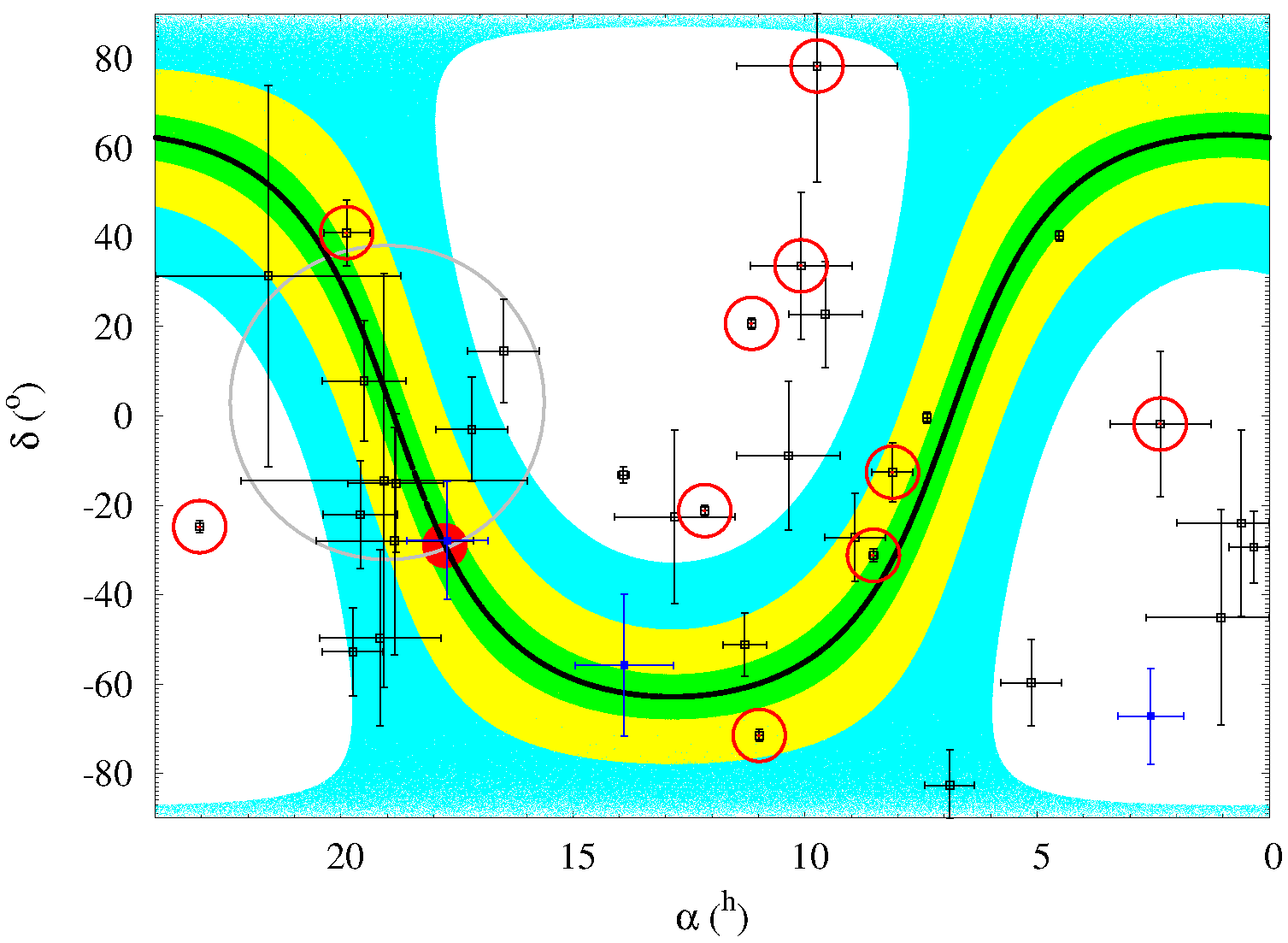
Figure 1: Distribution in equatorial coordinates (right ascension and declination) of 36 events observed by IceCube. Data and errors as in Supplementary Table 1 of Aartsen et al. (2014a). Events with deposited energies in excess of 1 PeV (3) appear in blue (filled squares), the others in black (empty squares). Events containing muon tracks can be identified by their much smaller positional error bars. The Galactic plane/equator appears as a continuous black line. The Galactic disk is arbitrarily defined as the region confined between galactic latitude $-5$and 5(in green). The position of the Galactic centre is represented by a filled red circle. The region enclosed between galactic latitude $-15$and 15appears in yellow, and the one confined by $-30$and 30in cyan. See Table 1 for the number of events found towards these regions. The large gray empty circle signals the approximate location of the Local Void. Event 18 is the leftmost one, event 10 is the rightmost one; both are well away from the bulk of the Galactic disk. Red empty circles signal probable background events (see the text for details).

It is widely accepted that the observed neutrinos come from two different sources, atmospheric and extraterrestrial. Atmospheric neutrinos are constantly being produced from all directions in the sky as they are the result of cosmic ray interactions in the upper atmosphere and subsequent decay of mesons; their deposited energies are expected to be under 100 TeV. The neutrino candidate events in Fig. 1 correspond to a deviation from the atmospheric background at the 5.7$\sigma$ level (Aartsen et al. 2014a). This means that out of 37 events, about 11 are background and the remaining 26 are extraterrestrial neutrinos. Aartsen et al. (2014a) already pointed out that the properties of events 3, 8, 18, 28 and 32 are consistent with them being background detections.

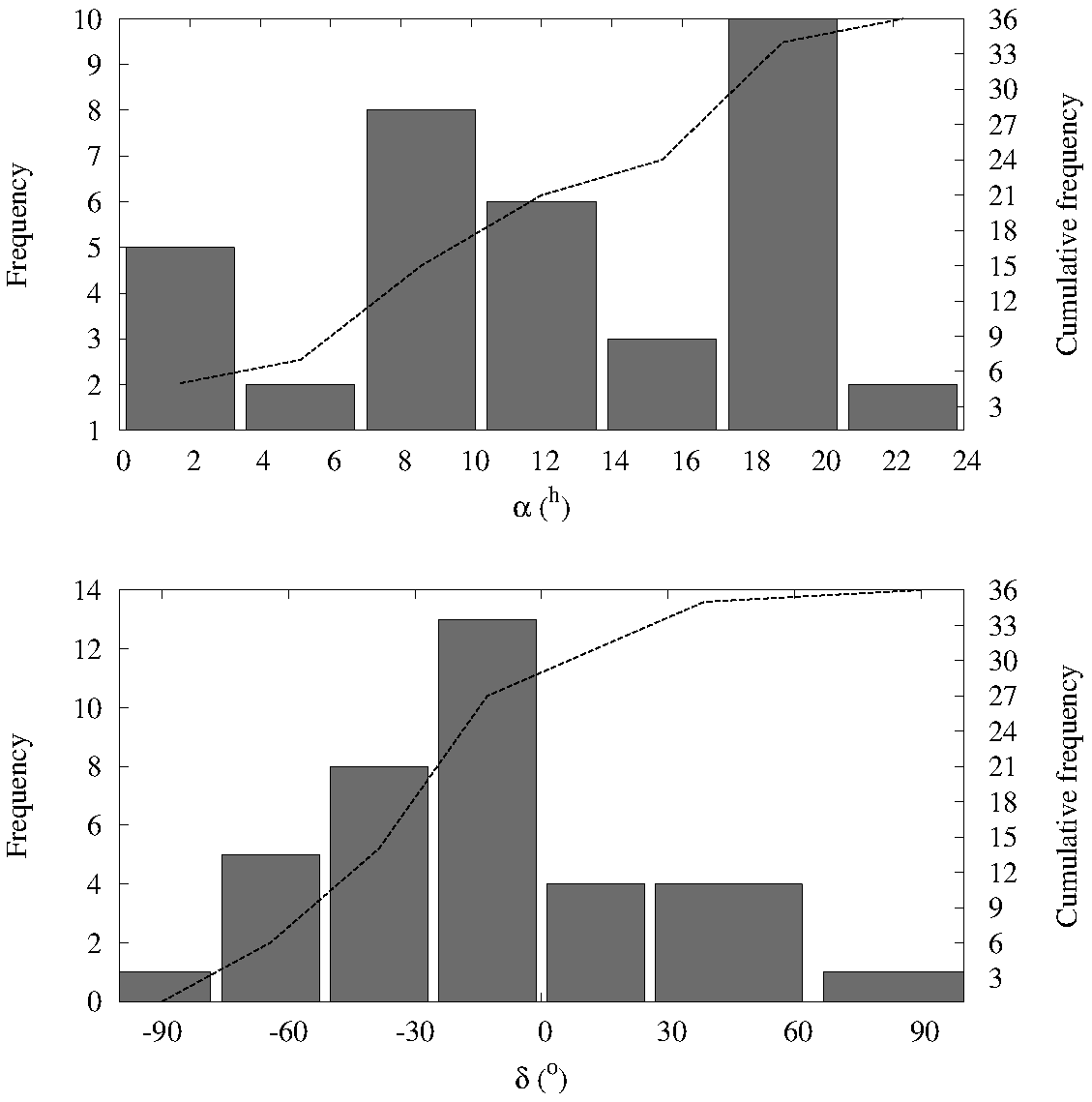
Figure 2: Frequency distribution in equatorial coordinates (right ascension, top panel, and declination, bottom panel) of the 36 neutrino candidate events that appear in Supplementary Table 1 of Aartsen et al. (2014a). The number of bins is 2 $n^{1/3}$ where $n=36$. An obvious excess of events in the right ascension range 8^h to 20^h is observed.

Figure 2 shows the frequency distribution in equatorial coordinates ($\alpha,\delta$) of the 36 neutrino candidate events discussed above. There is an obvious anisotropy in declination induced by the fact pointed out above that 27 events arrived from the southern celestial hemisphere. The source of this anisotropy is an observational bias, the IceCube neutrino observatory is more sensitive to events arriving from that direction. There is also an obvious excess of events in the right ascension range 8^h to 20^h. This range contains 27 events, outnumbering by 18 the 9 events in the ranges (0, 8)^h plus (20, 24)^h; this is a 4.2$\sigma$ departure from an isotropic distribution, where $\sigma=\sqrt{n}/2$ is the standard deviation for binomial statistics and $n$ is the number of events. It may be argued that the identified excess of neutrino candidate events towards the right ascension range 8^h to 20^h could be an effect of the instrumental acceptance. However, the Earth rotation guarantees the uniform exposure of the detectors in right ascension (Aguilar et al. 2013). If we focus on the 27 southern events, there are 18 of them within the right ascension range 8^h to 20^h and this still translates into a somewhat significant 2.45$\sigma$ departure from an isotropic distribution. Besides, this excess of neutrino candidate events towards the right ascension range 8^h to 20^h is consistent with the anisotropy in TeV cosmic rays identified by Schwadron et al. (2014).

In their study, Schwadron et al. (2014) have found a broad relative excess of cosmic rays between $\alpha\approx 8^{\rm h}$ and $\alpha\approx 18^{\rm h}$. The details of the observed anisotropy depend on the cosmic ray energy range considered. The relative excess in arrival direction is oriented towards the region of the sky that includes the downstream direction of the interstellar wind and the downfield direction of the Local Interstellar Magnetic Field (LIMF; Schwadron et al. 2014). These TeV cosmic ray anisotropies are related to the Interstellar Boundary Explorer (IBEX) ribbon (McComas et al. 2009). Neutrinos are not affected by the LIMF, but high-energy cosmic ray particles are and they can produce neutrinos when they interact with atomic nuclei creating unstable particles whose decay generates the neutrinos. As the parent high-energy cosmic ray particles can be deflected by magnetic fields, their original sources are almost impossible to trace. In this scenario, it is theoretically possible to produce extraterrestrial neutrinos at hundreds of AUs in the outskirts of the solar system; in fact, the structure observed by the IBEX spacecraft is a bright, narrow ($\sim$20wide) ribbon of energetic neutral atom emission that likely hints at the presence of an associated overdensity of matter. A putative production of neutrinos towards the edge of the solar system could further complicate the interpretation of the available data.

Figure 3 shows the location of the IBEX ribbon structure with respect to the Galactic equator and the IceCube events. The continuous yellow line follows the Local Interstellar Medium (LISM) magnetic equator as derived by Heerikhuisen et al. (2010). A 20 wide band around the LISM magnetic equator appears in pink. The IBEX ribbon is found within that area. Some events appear to be aligned along the band. As the arrival distribution of high energy cosmic rays appears to be affected by perturbations induced in the local interstellar magnetic field by the heliosphere wake (see, e.g., Desiati & Lazarian 2012; Schwadron et al. 2014) some of the detected neutrinos may have been generated in that region.

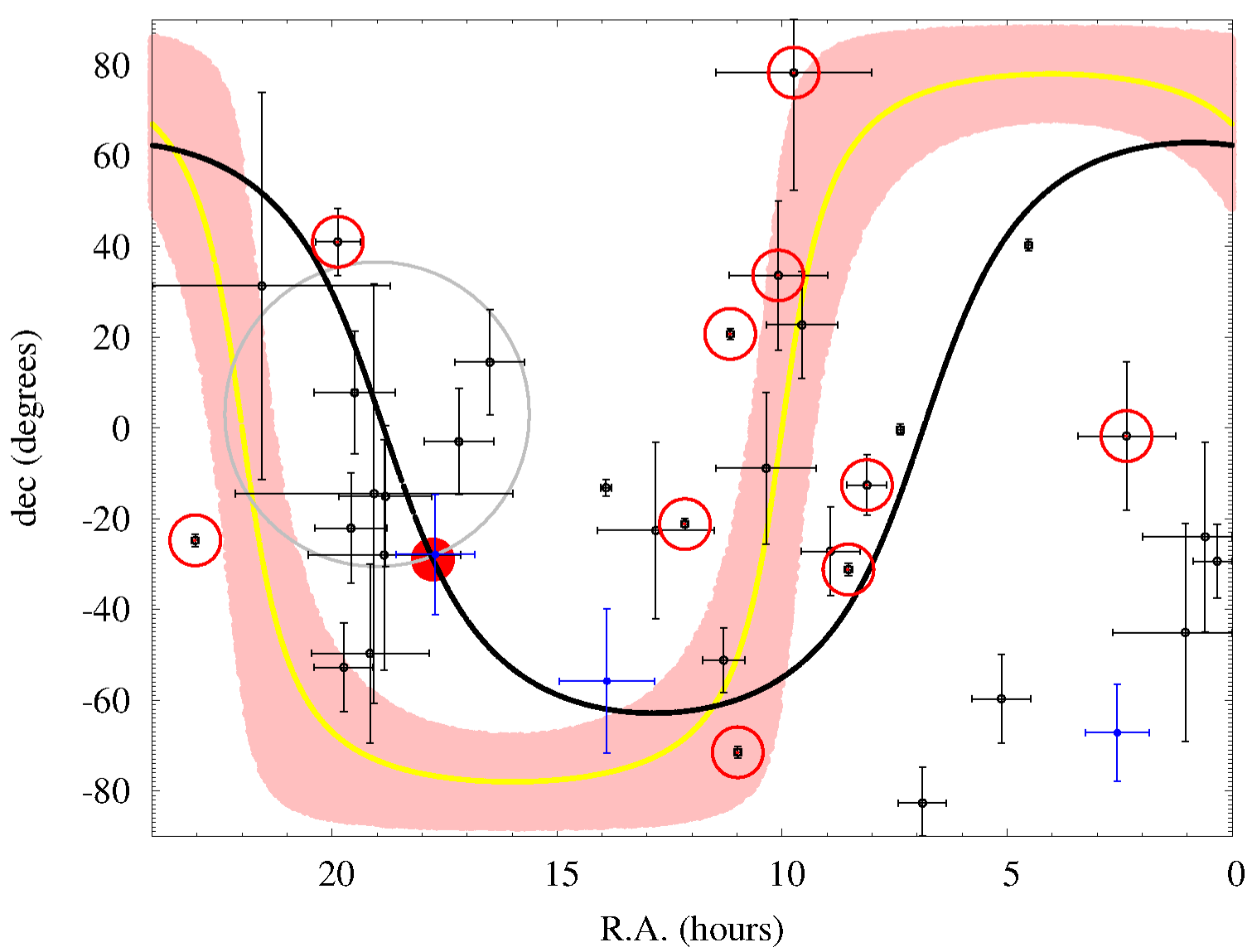
Figure 3: Distribution in equatorial coordinates (right ascension and declination) of 36 events observed by IceCube as plotted in Fig. 1. The Galactic plane appears as a continuous black line. The position of the Galactic centre is represented by a filled red circle. The large gray empty circle signals the approximate location of the Local Void. The continuous yellow line follows the LISM magnetic equator as derived by Heerikhuisen et al. (2010). A narrow ribbon ($\sim$20 wide) around the great circle defined by the LISM magnetic equator appears in pink. This area matches approximately the location of the IBEX ribbon (McComas et al. 2009).

Returning to the connection between neutrino candidate events and discrete sources, Bai et al. (2014) have provided robust evidence on the possible Sagittarius A^∗ origin of some of the events observed by IceCube. In particular, event 25 coincides spatially as well as temporally with some transient activity observed in X-rays towards Sagittarius A^∗ on 2012 February 9. Another notable spatial coincidence is the galaxy 2dFGRS TGS070Z303 and event 18 (a muon-track event), separated by just over 59 arcseconds. Galaxy 2dFGRS TGS070Z303 has a radial velocity of 37,866 km s^-1 (Colless et al. 2001). Also the galaxy 2dFGRS TGS280Z153 and event 10 (of shower-like topology) are separated by 218. Galaxy 2dFGRS TGS280Z153 has a radial velocity of 53,795 km s^-1 (Colless et al. 2001). An additional, perhaps significant, coincidence is the LINER AGN 2MASX J13550744-1309568 that is 516 from event 23, another muon-track event at coordinates $\alpha$ = 1391, $\delta=-$132. AGN 2MASX J13550744-1309568 has a radial velocity of 24,924 km s^-1 (Mauch & Sadler 2007).

3 A Monte Carlo-based angular distribution analysis

Let us consider a sample of $n$ events observed projected on the surface of a sphere, the sky in our case. We want to study the possible non-uniform spatial distribution of these events. In order to do that, we generate random points on the surface of a sphere using an algorithm due to Marsaglia (1972). The positions of these points on the sky have right ascension in the range (0^h, 24^h) and declination in the range (-90, 90). We perform 10⁷ experiments, each one including $n$ events, randomly distributed on the sky. In our histograms, the adopted number of bins is 2 $n_{\rm p}^{1/3}$, where $n_{\rm p}$ is the number of pairs. We compute the angular distance, $d$, between two given points (or events) using the equation $\cos d=\cos(\alpha_{1}-\alpha_{2})\cos\delta_{1}\cos\delta_{2}+\sin\delta_{1}\sin\delta_{2}$, where $(\alpha_{1},\delta_{1})$ and $(\alpha_{2},\delta_{2})$ are the equatorial coordinates of both points. Then count the number of pairs per bin and divide by the number of experiments performed.

The black continuous curves in Fig. 4 show the expected distribution of separations between events on the sky if they are uniformly distributed. The most probable separation is $\pi/2$ radians or 90. The distribution associated with the data in Supplementary Table 1 of Aartsen et al. (2014a) is far from regular (top panel) but only one bin deviates $\sim$2$\sigma$ (2.25$\sigma$) from a uniform distribution. Here, we use the approximation given by Gehrels (1986) when $n_{\rm p}<21$ to compute the error bars as Poisson statistics applies: $\sigma\sim 1+\sqrt{0.75+n_{\rm p}}$ ($\sigma=\sqrt{n_{\rm p}}$ otherwise), where $n_{\rm p}$ is the number of pairs. In principle, all the events are uncorrelated and distributed according to Poisson statistics. The addition of two independent Poissonian variables (considering terrestrial and extraterrestrial events, see above) is still Poissonian.

Figure 4, top panel, does not take into account the fact that a fraction of the events (11 out of 37) likely have terrestrial origin. Only the extraterrestrial neutrinos are of interest here, i.e. the sample must be decontaminated. Background rejection is implemented following the conclusions obtained by Aartsen et al. (2014a), and also using an algorithm in which we assume that they will have deposited energies under 100 TeV and that (approximately and based on Fig. 2 in Aartsen et al. 2014a) 8 background events have energies in the range 30–53.3 TeV, 2 in the range 53.3–76.7 TeV, and 1 in the range 76.7–100 TeV. In addition, we rank events based on how high is their probability of being part of an isotropic distribution. At the energies of interest here, the angular distribution of atmospheric neutrinos is expected to be very nearly isotropic. We compute the separation distributions for all the possible combinations (more than 600 million) of 11 events and compare with that of an isotropic distribution of the same size. Those combinations of 11 events with root-mean-square deviation from the isotropic behaviour $<$ 0.0047 are selected and the number of times each event appears is counted. Statistically speaking, those with the highest number of counts are more likely to be part of an isotropically distributed subsample. Using the conclusions from Aartsen et al. (2014a) and the events ranked as described, we conclude that the most probable background events are: 1, 3, 8, 9, 18, 27, 28, 29, 31, 32 and 37. These events appear as red empty circles in Fig. 1 (for a different approach to the issue of background rejection see Padovani & Resconi 2014).

If we focus on the 26 events (or 325 pairs) which are most probably of extraterrestrial origin, we obtain the bottom panel in Fig. 4. For this decontaminated sample, the difference between the theoretical (isotropic) value and the actual one is always $<2.5\sigma$. However, the range 0 to $\pi$/2 radians contains 195 pairs, outnumbering by 65 the 130 pairs in the range $\pi$/2 to $\pi$ radians; this is a 3.6$\sigma$ departure from an isotropic distribution, where $\sigma=\sqrt{n_{\rm p}}/2$ is now the standard deviation for binomial statistics. Therefore, the irregular distribution on the celestial sphere is different from that of a sample of points uniformly scattered, i.e. an anisotropy exists. An excess of events appears to be located towards the equatorial coordinates (187, $-23$); this has already been pointed out by Aartsen et al. (2013c). This region is relatively far from the Galactic disk, the densest part of the Milky Way Galaxy, and towards the Local Void (Tully & Fisher 1987). This area of the sky has a confirmed low local density of galaxies with radial velocities below 3,000 km s^-1 (see, e.g., Fig. 2 in Nasonova & Karachentsev 2011). This region of low density extends up to distances of 40 to 60 Mpc centred at least 23 Mpc from the Milky Way (Tully et al. 2008) and it may be even larger, perhaps connecting with the Microscopium/Sagittarius void (Kraan-Korteweg et al. 2008). The geometric centre of the Local Void is found towards the equatorial coordinates (190, +3), starting at the edge of the Local Group (Nasonova & Karachentsev 2011). The large gray empty circle in Fig. 1 signals the approximate location and projected extension of the Local Void. Taking into account the error bars, it encloses nearly 25% of all the IceCube events.

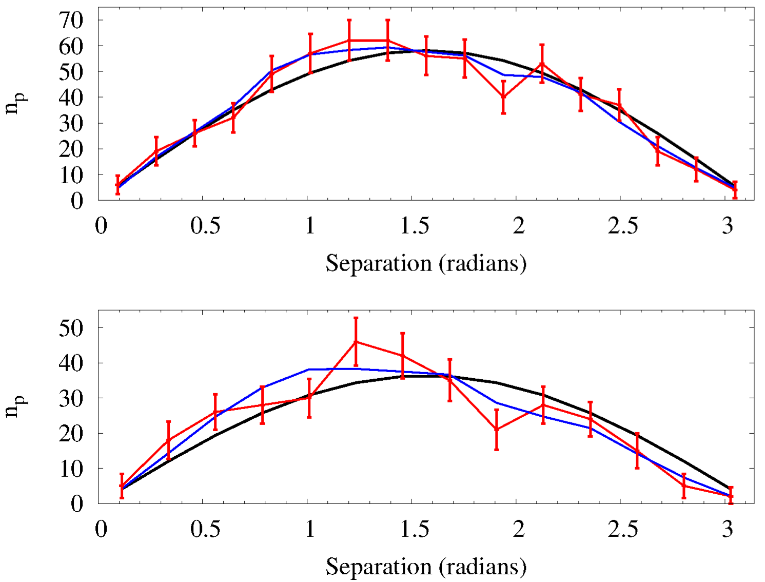
Figure 4: Separation distribution for the events in Supplementary Table 1 of Aartsen et al. (2014a), red line/points with error bars, the number of pairs is $n_{\rm p}$. The theoretical separation distribution for an uniformly spread sample across the sky of $n$ = 36 events (or 630 pairs, top panel) and $n$ = 26 events (or 325 pairs, bottom panel) is displayed as a continuous black line. The top panel displays the entire sample of 36 events and the bottom panel shows the results excluding events of probable terrestrial origin, a subsample of 26. The blue lines correspond to the average separation distribution when the positional errors associated with the events are taken into account (see the text for details). The 1$\sigma$ error bars have been computed as described in the text. The number of bins is 2 $n_{\rm p}^{1/3}$.

On the other hand, the Galactic disk is the brightest source of gamma rays in the sky, can the excess of events pointed out above have their origin in the disk? To test this hypothesis we count the number of IceCube events within bands whose boundaries are limited in galactic latitude, $b$ (see Table 1). For example, points within the Galactic disk have $|\Delta b|$ = 5and are confined between galactic latitude $-5$and 5(green area in Fig. 1). We repeat the process using the same uniformly distributed model studied before. Differences between the observational data and the isotropic model are not statistically significant. It appears unlikely that the dominant source of these high-energy neutrinos is in or near the Galactic disk. This is somewhat consistent with results obtained by Aartsen et al. (2014a); in their work, it is found that the correlation with the Galactic plane is not significant, with a probability of 2.8% for a width of the disk of $\pm$75. Restricting the analysis to the range of right ascension 16^h to 22^h does not show any significant changes and that also makes the Galactic bulge an unlikely source. Results are equivalent for the full sample and the decontaminated one (see Table 1, in boldface).

Table 1: Number of events detected by IceCube as a function of the galactic latitude, $b$, or distance from the Galactic plane in steps of 5and the expected number of events derived from an isotropic model (see the text) with its associated error. The difference between the observational data and the isotropic model in units of $\sigma$ is also given. Results for the decontaminated sample appear in boldface. See Fig. 1 for a reference on the various $|\Delta b|$ regions.

$|\Delta b|$ ()	isotropic ($\pm\sigma$)	IceCube data	Difference (in units of $\sigma$)
5	3.14$\pm$2.97	3	0.05
	2.27$\pm$2.74	2	0.10
10	6.25$\pm$3.65	10	1.03
	4.51$\pm$3.29	8	1.06
15	9.32$\pm$4.17	15	1.36
	6.73$\pm$3.73	11	1.14
20	12.31$\pm$4.61	16	0.80
	8.89$\pm$4.10	12	0.75
25	15.21$\pm$4.99	18	0.56
	10.98$\pm$4.42	14	0.68
30	18.00$\pm$5.33	20	0.38
	13.00$\pm$4.71	16	0.64

Our previous analysis has not taken into consideration that the positional errors associated with the events, in particular to those of shower topology, are very large, much larger than those typical of optical astrometry. What is the impact of these errors on our previous analysis? In order to evaluate the effect of large angular errors on the separation distribution, we generate sets of synthetic events Monte Carlo-style (Metropolis & Ulam 1949) using the equatorial coordinates and median angular errors in Supplementary Table 1 of Aartsen et al. (2014a). For a given event of coordinates $(\alpha,\delta)$ and median angular error $\Delta e$, we generate a synthetic event of coordinates $(\alpha_{\rm s},\delta_{\rm s})$ where the new coordinates are such that the angular distance between the synthetic coordinates and the original ones is given by $d^{*}=|{\rm GRND}|\ \Delta e$, with GRND being a random number in the interval (-1, 1) following a Gaussian distribution obtained using the Box-Muller method (Press et al. 2007) with zero mean and unit variance. If the North Celestial Pole is within the error circle, declination is restricted to the range $\delta-\Delta e$ to $+\pi$/2, when the South Celestial Pole is included the declination range is $-\pi$/2 to $\delta+\Delta e$; in both cases, the right ascension can take any value in the range 0^h to 24^h as parts of all meridians are within the error circle as well. This approach is not singular at the poles. When none of the poles is included within the error circle, the range in declination is $\delta-\Delta e$ to $\delta+\Delta e$ and the equivalent in right ascension is $\alpha-\Delta e$ to $\alpha+\Delta e$. The average separation distribution for 10⁷ sets of synthetic events based on the original ones and their positional errors is displayed as a blue line in Fig. 4 (top panel). Taking into account the positional errors significantly reduces the difference between the observational angular separation distribution and that of an isotropic case. However, for the clean sample (bottom panel) there is still a 3.1$\sigma$ departure from an isotropic distribution when considering separations smaller than $\pi$/2. The approach outlined here has also been used to strengthen the results of our decontamination algorithm (see above) and our list of most probable background events has been obtained after hundreds of trials that use the median angular errors.

4 The atmospheric background

The background produced by atmospheric neutrinos is of diffuse nature. These atmospheric neutrinos result from cosmic rays interacting with the atmosphere. So far, our analysis has assumed that this background follows a mathematically isotropic model as the theory predicts. However, in the calculations carried out by the IceCube collaboration, the significance of their results is evaluated by comparing with a distribution obtained by performing yet another analysis over a sample of only-background data sets that are obtained by scrambling real data in right ascension. In other words, right ascension is randomized while keeping the original values in declination. This is done to take into account that the detector has anisotropic acceptance, i.e. its instrumental response function is unknown. This approach assumes that the unknown instrumental response function does not change over time, i.e. it remains the same over the entire search period. Figure 5 shows that under this approach the separation distribution of the 27 southern events and that of an average of $10^{7}$ only-background data sets are compatible, i.e. the angular distribution of the events is isotropic. However, deviations close to 1.5$\sigma$ are observed.

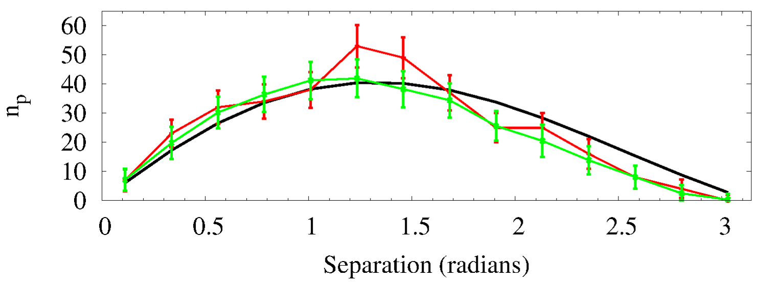
Figure 5: Separation distribution (red line/points with error bars, top panel) for the 27 events located towards the southern hemisphere (negative declination) in Supplementary Table 1 of Aartsen et al. (2014a), the number of pairs is $n_{\rm p}$. The analogous separation distribution for an uniformly distributed sample across a semisphere of $n$ = 27 events or 531 pairs is displayed as a continuous black line. The continuous green line shows the average of $10^{7}$ experiments where the right ascension is randomized as described in the text.

5 Discussion

After being emitted, neutrinos move unaffected by gas, dust or magnetic fields. The somewhat significant excess observed towards the equatorial coordinates (187, $-23$) is an important clue to the origin of the observed events as their associated neutrinos have travelled very little distance (if their sources are Galactic) or across mostly empty space in their final leg, the Local Void (if they are of extragalactic origin). This is probably the key fact to understand the place of origin of the majority of events detected so far by the IceCube neutrino observatory, extragalactic versus local. Our analysis shows no statistically significant excess of events associated with the Galactic disk (see above). If sources in the Galactic halo are expected to follow a uniform spread, then our findings are somewhat incompatible with such origin. As for sources within the Local Group, multiple events are observed towards an area of the sky where the density of galaxies with radial velocities below 3,000 km s^-1 is quite low. The alternative explanation is straightforward: sources located at cosmological distances, well beyond the Local Group.

The spatial distribution of galaxies situated at cosmological distances has been found to be hierarchical (see, e.g., Pietronero 1987) and this is also consistent with numerical expectations since early studies (e.g. Aarseth et al. 1979). In an attempt to further explore this interesting possibility, a dominant extragalactic origin for these events, we restrict our analysis to the sample of 27 events located towards the southern hemisphere in Supplementary Table 1 of Aartsen et al. (2014a). The separation distribution of this subsample (on the surface of a semisphere) is quite different from that in Fig. 4, with a reduced number of pairs separated by more than $\pi/2$ radians (the average angular distance for points uniformly spread on a sphere) with respect to the full sample (see Fig. 6).

In order to check if the angular distribution of events on the semisphere is isotropic, we proceed as we did with the full sample and perform 10⁷ experiments, each one including 27 events randomly distributed on the southern half of the celestial sphere, counting the number of pairs within a certain range of separations. The results are plotted as a black continuous line in Fig. 6. Differences between the uniform case and the subsample are consistent across the entire separation range and they are marginally significant for some bins (the largest difference is 1.8$\sigma$). Our analysis shows that, for events observed towards the southern hemisphere, the angular distribution is not isotropic. There is a 3.7$\sigma$ departure from an isotropic distribution when considering separations smaller than $\pi$/2; as pointed out above, the deviation for the entire celestial sphere is 3.6$\sigma$. If we replace the original set of 27 data by sets of synthetic events obtained from the original ones and their Gaussian positional errors (see above) and average the results of 10⁷ experiments, we obtain the blue curve in Fig. 6 (top panel) that deviates even more clearly from the isotropic arrival scenario (black curve) for separations larger than the average (the largest difference is now close to 3$\sigma$ near the high end of the distribution). We observe 98 pairs with angular separation in the range $\pi$/2 to $\pi$ instead of the expected 149 in the isotropic case, a 5.5$\sigma$ deviation. This reduced number of pairs characterized by large separations strongly favours the existence of some type of weak but noticeable clustering for these neutrino sources. Absence of strong anisotropy is usually interpreted as an indication of cosmological origin. Using the decontaminated sample (see Fig. 6, bottom panel), we observe a 3.9$\sigma$ departure (149 observed pairs instead of 121 in the isotropic case for a total of 210 pairs) from an isotropic distribution when considering separations smaller than $\pi$/2. When taking into account the positional errors the statistical significance is reduced to 2.8$\sigma$.

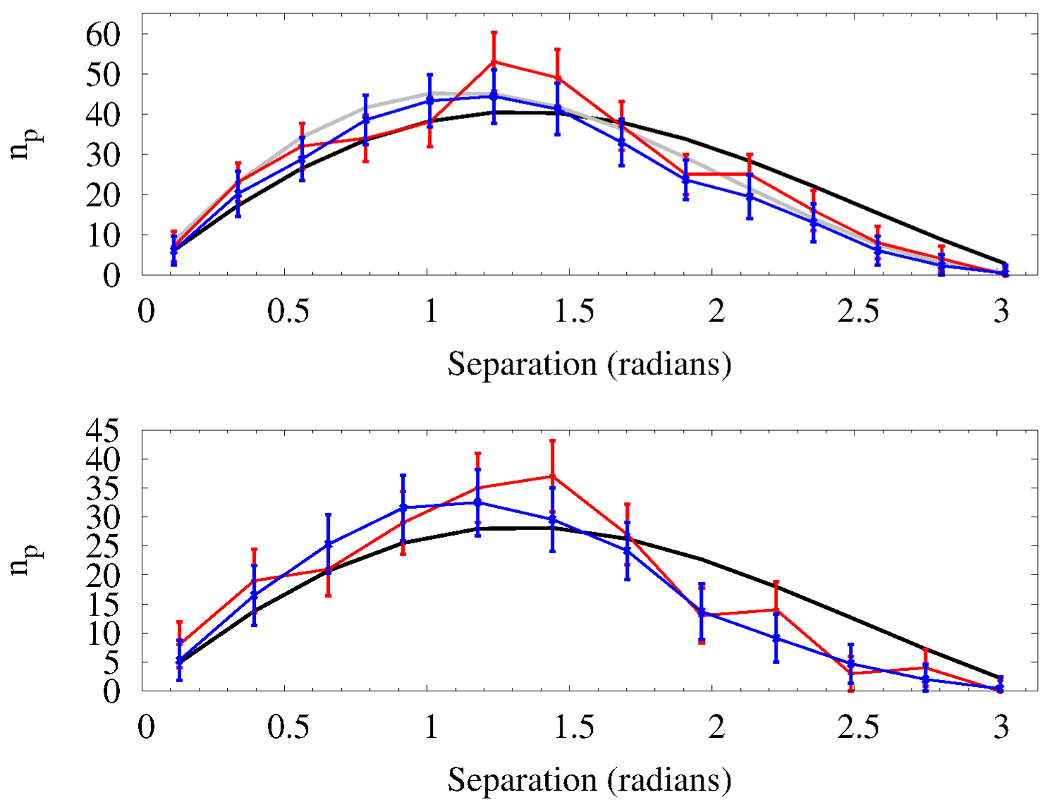
Figure 6: Separation distribution (red line/points with error bars, top panel) for the 27 events located towards the southern hemisphere (negative declination) in Supplementary Table 1 of Aartsen et al. (2014a), the number of pairs is $n_{\rm p}$. The analogous separation distribution for an uniformly distributed sample across a semisphere of $n$ = 27 events or 531 pairs is displayed as a continuous black line in both panels. The average separation distribution for a set of synthetic events obtained from the original events and their Gaussian positional errors appears as a blue line, the average number of synthetic events is $\sim$25.8 and the associated number of pairs is $\sim$319.9, more details in the text. The gray line shows the best fractal-like distribution (see the text for details). The bottom panel plots the equivalent results for the decontaminated sample of 21 events. The 1$\sigma$ error bars have been computed as described in the text. The number of bins is 2 $n_{\rm p}^{1/3}$, where $n_{\rm p}$ is 531 (top) and 210 (bottom).

If the sources of these neutrinos are located at cosmological distances, probably within remote galaxy clusters, one may expect that they are organized following a hierarchical fractal model. Star formation within the Milky Way follows a fractal pattern (e.g. de la Fuente Marcos & de la Fuente Marcos 2006a); similar patterns are observed in starburst galaxies (e.g. de la Fuente Marcos & de la Fuente Marcos 2006b,c). Soneira & Peebles (1978) showed that the appearance of the projected distribution of galaxies can be reproduced using a model based on the superposition of fractal clumps. In order to test this hipothesis we consider $n_{\rm a}$ uniformly distributed points, $(\alpha_{n},\delta_{n})$, on the surface of the unit semisphere. Each point is the centre of an arc of radius $R/\lambda$. Within each arc we consider $n_{\rm a}$ additional uniformly distributed points, each one is centre for an associated arc of radius $R/\lambda^{2}$. Within each arc and on the surface of the unit semisphere, we generate $n_{\rm a}$ uniformly distributed points. The approach is similar to the one described by Soneira & Peebles (1978).

In our case, and in order to have 27 points (events) per experiment, we consider $n_{\rm a}$ = 3, $R$ in the range $\sim$0 to $\sim 2\pi$ and $\lambda\in(0,2)$. After performing a large number of tests, each one consisting of 10⁶ experiments, the best fit to the southern hemisphere data is found for $R=\pi$ and $\lambda=0.9$. The gray curve in Fig. 6, top panel, shows the distribution of separations for our fractal-like model. Although unable to reproduce the asymmetric behaviour at separations in the range 0.5-1.5 radians (top panel), its deviations from the actual data are not statistically significant and its overall agreement improves for the average separation distribution of synthetic events (blue curve in Fig. 6, top panel). These deviations are always smaller than those from a uniform distribution. In order to find out how significant the differences between the two models (fractal-like versus isotropic) are and because the sample is rather small, we use the likelihood formula due to Saha (1998). The average value of the $W$ estimator for the fractal-like model is 6 times greater than the one for the isotropic model; therefore, it is statistically more robust. The distribution of events over the southern hemisphere is almost certainly anisotropic.

6 Conclusions

In this paper, we have studied the angular distribution of IceCube high-energy events trying to answer the astrophysically relevant question of whether or not their spread is isotropic to conclude that the observed events are very probably not evenly distributed on the sky. Differences between a uniform angular distribution and the observed one are indeed marginally significant at the 2$\sigma$ level or better. Our main findings can be summarized as follows:

• The angular distribution of IceCube high-energy events exhibits a modest but statistically significant anisotropy.

• There is no statistically significant excess of events projected towards the Galactic disk.

• The observed distribution of events appears to be incompatible with an origin in the Milky Way halo.

• A relatively significant excess of events appears projected towards the Local Void. This suggests either a Galactic origin or one well beyond the Local Group for these events.

• The angular distribution of events towards the southern hemisphere appears to be anisotropic and it is statistically more compatible with an origin in a distant, fractal-like organized structure than with the currently assumed isotropicity.

We must stress that our results are based on small number statistics. However, they are compatible with well-established results for GRBs, namely that short GRBs are distributed anisotropically (Balázs et al. 1998). Anisotropy is also observed for the highest energy cosmic rays (e.g. Abreu et al. 2012; Schwadron et al. 2014). Because of the small size of the current data set compared to those of short GRBs or high-energy cosmic rays, the results of our study are necessarily limited in scope as only very large effects can be reliably identified. Although a small fraction of closer sources is possible (perhaps those putatively related to the IBEX ribbon), remote hierarchical structures appear to be the main source of these energetic neutrinos.

- [1] Aarseth, S.J., Turner, E.L., & Gott, J.R. III 1979, ApJ, 228, 664
- [2] Aartsen, M.G., Abbasi, R., Abdou, Y., et al. (IceCube Coll.) 2013a, Sci, 342, 1242856
- [3] Aartsen, M.G., Abbasi, R., Abdou, Y., et al. (IceCube Coll.) 2013b, Phys. Rev. Lett., 111, 021103
- [4] Aartsen, M.G., Abbasi, R., Ackermann, M., et al. (IceCube Coll.) 2013c, Phys. Rev. D, 88, 112008
- [5] Aartsen, M.G., Ackermann, M., Adams, J., et al. (IceCube Coll.) 2014a, Phys. Rev. Lett., 113, 101101
- [6] Aartsen, M.G., Ackermann, M., Adams, J., et al. (IceCube Coll.) 2014b, ApJ, 796, 109
- [7] Abreu, P., Aglietta, M., Ahlers, M., et al. 2012, J. Cosmol. Astropart. Phys., 4, 40
- [8] Aguilar, J.A., Aartsen, M.G., Abbasi, R., et al. (IceCube Coll.) 2013, Nuclear Physics B - Proceedings Supplements, 239–240, 184 (arXiv:1010.6263)
- [9] Ahlers, M., & Murase, K. 2014, Phys. Rev. D, 90, 023010
- [10] Anchordoqui, L.A., Goldberg, H., Lynch, M.H., et al. 2014a, Phys. Rev. D, 89, 083003
- [11] Anchordoqui, L.A., Paul, T.C., da Silva, L.H.M., Torres, D.F., & Vlcek, B.J. 2014b, Phys. Rev. D, 89, 127304
- [12] Arnett, W.D., Bahcall, J.N., Kirshner, R.P., & Woosley, S.E. 1989, ARA&A, 27, 629
- [13] Bahcall, J.N. 2005, Phys. Scr., T121, 46
- [14] Bai, Y., Barger, A.J., Barger, V., et al. 2014, Phys. Rev. D, 90, 063012
- [15] Balázs, L.G., Mészáros, A., & Horváth, I. 1998, A&A, 339, 1
- [16] Becker Tjus, J., Eichmann, B., Halzen, F., Kheirandish, A., & Saba, S.M. 2014, Phys. Rev. D, 89, 123005
- [17] Bellerive, A. 2004, Int. J. Mod. Phys. A, 19, 1167
- [18] Bhattacharya, A., Choubey, S., Gandhi, R., & Watanabe, A. 2010, J. Cosmol. Astropart. Phys., 9, 9
- [19] Chen, C.-Y., Dev, P.S.B., & Soni, A. 2014, Phys. Rev. D, 89, 033012
- [20] Colless, M., Dalton, G., Maddox, S., et al., 2001, MNRAS, 328, 1039
- [21] de la Fuente Marcos, R., & de la Fuente Marcos, C. 2006a, A&A, 452, 163
- [22] de la Fuente Marcos, R., & de la Fuente Marcos, C. 2006b, A&A, 454, 473
- [23] de la Fuente Marcos, R., & de la Fuente Marcos, C. 2006c, MNRAS, 372, 279
- [24] Desiati, P., & Lazarian, A. 2012, ApJ, 762, 44
- [25] Ema, Y., Jinno, R., & Moroi, T. 2014, Phys. Lett. B, 733, 120
- [26] Gehrels, N. 1986, ApJ, 303, 336
- [27] Halzen, F. 2014, Astron. Nachr., 335, 507
- [28] Heerikhuisen, J., Pogorelov, N.V., Zank, G.P., et al. 2010, ApJ, 708, L126
- [29] Joshi, J.C., Winter, W., & Gupta, N. 2014, MNRAS, 439, 3414
- [30] Kraan-Korteweg, R.C., Shafi, N., Koribalski, B.S., et al. 2008, Outlining the Local Void with the Parkes HI ZOA and Galactic Bulge Surveys, in Galaxies in the Local Universe, ed. B.S. Koribalski, & H. Jerjen, Springer Netherlands, Astrophysics and Space Science Proceedings, 13
- [31] Krauß F., Kadler, M., Mannheim, K., et al. 2014, A&A, 566, L7
- [32] Liu, R.-Y., Wang, X.-Y., Inoue, S., Crocker, R., & Aharonian, F. 2014, Phys. Rev. D, 89, 083004
- [33] Lunardini, C., Razzaque, S., Theodoseau, K.T., & Yang, L. 2014, Phys. Rev. D, 90, 023016
- [34] Marsaglia, G. 1972, Ann. Math. Stat., 43, 645
- [35] Mauch, T., & Sadler, E.M. 2007, MNRAS, 375, 931
- [36] McComas, D.J., Allegrini, F., Bochsler, P., et al. 2009, Sci, 326, 959
- [37] Metropolis, N., & Ulam, S. 1949, J. Am. Stat. Assoc., 44, 335
- [38] Murase, K., Ahlers, M., & Lacki, B.C. 2013, Phys. Rev. D, 88, 121301
- [39] Nasonova, O.G., & Karachentsev, I.D. 2011, Astrophys., 54, 1
- [40] Padovani, P., & Resconi, E. 2014, MNRAS, 443, 474
- [41] Pietronero, L. 1987, Physica A, 144, 257
- [42] Press, W.H., Teukolsky, S.A., Vetterling, W.T., & Flannery, B.P. 2007, Numerical Recipes: The Art of Scientific Computing, 3rd Edition (Cambridge Univ. Press, Cambridge), 364
- [43] Razzaque, S. 2013a, Phys. Rev. D, 88, 081302
- [44] Razzaque, S. 2013b, Phys. Rev. D, 88, 103003
- [45] Saha, P. 1998, AJ, 115, 1206
- [46] Schwadron, N.A., Adams, F.C., Christian, E.R., et al. 2014, Sci, 343, 988
- [47] Soneira, R.M., & Peebles, P.J.E. 1978, AJ, 83, 845
- [48] Taylor, A.M., Gabici, S., & Aharonian, F. 2014, Phys. Rev. D, 89, 103003
- [49] Tully, R.B., & Fisher, J.R. 1987, Nearby Galaxies Atlas (Cambridge Univ. Press, Cambridge)
- [50] Tully, R.B., Shaya, E.J., Karachentsev, I.D., et al. 2008, ApJ, 676, 184
- [51] Winter, W. 2013, Phys. Rev. D, 88, 083007
- [52] Zavala, J. 2014, Phys. Rev. D, 89, 123516