Odd frequency pairing of interacting Majorana fermions

Abstract

Majorana fermions are rising as a promising key component in quantum computation. While the prevalent approach is to use a quadratic (i.e. non-interacting) Majorana Hamiltonian, when expressed in terms of Dirac fermions, generically the Hamiltonian involves interaction terms. Here we focus on the possible pair correlations in a simple model system. We study a model of Majorana fermions coupled to a boson mode and show that the anomalous correlator between different Majorana fermions, located at opposite ends of a topological wire, exhibits odd frequency behavior. It is stabilized when the coupling strength $g$ is above a critical value $g_{c}$. We use both, conventional diagrammatic theory and a functional integral approach, to derive the gap equation, the critical temperature, the gap function, the critical coupling, and a Ginzburg-Landau theory allowing to discuss a possible subleading admixture of even-frequency pairing.

Introduction

Recent advances in material fabrication techniques have brought Majorana fermions out of a theoretician’s toy box and placed them onto the stage of realistic objects. Majorana fermions are particles with the peculiar property of being their own anti-particles. While its status as a fundamental particle is still unclear in the arena it was first proposed, namely neutrino in particle physics, in condensed matter physics, on the other hand, there have been realistic proposals and indeed fairly convincing experimental signatures that these will come into existence as zero energy modes Kitaev (2001); Alicea (2012); Cheng et al. (2010); Rokhinson et al. (2012); Wilczek (2009); Mourik et al. (2012); Churchill et al. (2013); Wang et al. (2014). Apart from the obvious theoretical interest, such Majorana zero modes are particularly attractive as a potential key component in topological quantum computation Kitaev (2003); Nayak et al. (2008); Beenakker (2013) because their origin is often of a topological nature (vortices, end modes, topological Dirac materials, etc.), hence their existence is robust and protected against disruptions such as defects, perturbations and decoherence. Since they also exhibit anyonic statistics under suitable conditions, their mutual braiding would constitute the fundamental operation to encode and process information. They are thus well suited for fault-tolerant quantum computation.

While Majorana fermions are most often studied using an effective Hamiltonian bilinear in Majorana operators, the fundamental object in the condensed matter context, however, is still Dirac fermions. These effective Hamiltonians, when written in terms of Dirac fermions, generically contain both particle ($c^{\dagger}c$) and pairing ($cc$) terms, which is why any condensed matter platform for Majorana fermions necessarily contains superconductivity Wilczek (2009). As pairing inevitably arises from interaction, an important question one should ask is what types of instability would ensue. For conventional fermions and bosons, such instabilities would generate non-vanishing anomalous correlation functions which represent the onset of steady orders such as charge, spin, or pair susceptibilities. The same can be done for Majorana fermions Asano and Tanaka (2013); Liu et al. (2015). The effective Hamiltonian formalism, being time-independent in its nature, implicitly assumes that these instabilities are dominated by their equal time behavior (i.e. the even-in-time component). However, the very nature of Majorana fermions being simultaneously a particle and an anti-particle hints to the possibility that time (or frequency) dependence in the order parameter has a fundamental role to play. As a heuristic example, the pairing correlator $M_{\tau}\equiv\langle\mathcal{T}\mu(\tau)\mu(0)\rangle$ of Majorana operator $\mu$ separated by (Matsubara) time $\tau$ is forced to be odd in time, and therefore vanishes at equal time. A more complete discussion on the pairing symmetries of Majorana fermions will be presented later.

Historically, an odd frequency (odd-f) pairing state was first pointed out by Berezinskii Berezinskii (1974) in 1974 as a candidate state for superfluid He3. While this was eventually proven not to be the case, Berezinskii’s pioneering paper set the stage for subsequent searches of other possible odd-f states, such as spin singlet odd-f pairing state Balatsky and Abrahams (1992); Belitz and Kirkpatrick (1992). Although initial search of models and systems realizing such states turned out to be inconclusive Abrahams et al. (1995), more recent discussions of odd-f states have moved to systems of superconducting heterostructures where one can have conventional pairs converted into odd-f states at the interfaces Bergeret et al. (2005); Tanaka et al. (2012); Burset et al. (2015); Ebisu et al. (2015). Moreover, odd-f states can also be realized in homogeneous multiband superconductors Black-Schaffer et al. (2013); Black-Schaffer and Balatsky (2013). If we take the broader view that odd-f states represent a novel class of hidden order, then this concept may be extended beyond superconductivity to encompass a whole set of states that might have odd-f order parameters Abrahams et al. (1995); Bergeret et al. (2005); Tanaka et al. (2012), e.g., spin nematics Balatsky and Abrahams (1995), BEC Balatsky (2014), and density waves Kedem and Balatsky (2015).

In this work, we will study pairing of Majorana fermions in the presence of interaction induced by coupling to an external boson. Our focus will be on the pairing between different Majorana modes because it arises solely as a consequence of interaction. Unlike same-mode pairing which, as discussed before, is required to be odd-f due to fermionic statistics, there is no a priori requirement on the frequency dependence for cross-mode Majorana pairing. Indeed, as we will show, both even-f and odd-f solutions exist for the gap equation, yet the odd-f solution has a lower free energy and is hence more stable than the even-f state. We determine the phase diagram in the temperature-coupling constant plane showing the disordered high temperature phase and a pair-correlated low-temperature phase, separated by a second-order transition. Interestingly, we find a quantum phase transition at a critical coupling, in contrast to conventional BCS theory where any weak attractive interaction induces pairing, if only at an exponentially small temperature. We derive the gap equation and solve it both, analytically in the limit of high and low temperature, and numerically. The critical coupling at low $T$ may be linked to the first excited state of an effective Schrödinger equation, enabling a determination of the critical coupling. We also derive a functional integral representation of the partition function in terms of the pair order field, which allows to estimate the condensation energy. The latter may also be used to derive an approximate Ginzburg-Landau expansion in terms of both, the odd- and even-frequency order parameters.

Majorana pairing state and Extension of Berezinskii’s classification

To set the stage, first consider the notion of pairing state. A state is paired when any two-particle anomalous expectation is finite: for any particle operator $O^{a}(r,\tau)$, where $a$ denotes a collective quantum number, its pairing amplitude is

$$P_{O}^{ab}(r,\tau)=\langle\mathcal{T}O^{a}(r,\tau)O^{b}(0,0)\rangle$$ (1)

The cases of fermions $O(r,\tau)=c(r,\tau)$ , spins $O^{a}(r,\tau)=S^{a}(r,\tau)$ ($a$ denoting directions), and boson $O^{a}(r,\tau)=b_{a}(r,\tau)$ ($a$ denoting, say, species) all fall within the category of thus defined paired states. This does not necessarily mean there is a true superconducting or superfluid order. For example, a typical pairing state that supports a superflow would exhibit a $U(1)$ gauge symmetry breaking related to phase coherence and off-diagonal long range order, and has other attributes like phase stiffness. We instead accept that thus defined pairing correlation is the basic property that we investigate in the context of Majorana fermions. Since Majorana operators are real, the only symmetry left to be broken is $Z_{2}$ symmetry. Thus there are important distinctions between the “paired” Majorana states and conventional pairing. Yet the question about the appearance of anomalous order in models with Majorana states stands and needs to be addressed. We focus on the pairing correlator as a fundamental ingredient that any “super” state must possess – such correlations might be important indicators of incipient orders.

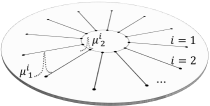
Figure 1: Schematics of superconducting wires that host Majorana fermions $\mu^{i}_{a}$ on their edges, where $i$ is the wire index and $a=1,2$ labels the edge. Dashed line illustrates possible coupling between Majorana fermions on neighboring wires.

We start with the extension of the Berezinskii classification for Majorana operators. Consider a set of Majorana states that emerge from materials like the ends of magnetic or semiconducting wires, see Fig. 1. We introduce Majorana operators

$$\mu_{a}^{i}=(\mu_{a}^{i})^{{\dagger}}\quad,\quad i=1...N\ ,\ a=1,2\ ,$$ (2)

where $i$ is the wire index and $a$ denotes the two ends of the wire. Following Eq. 1, consider the matrix of pair amplitudes

$$M_{ab}^{ij}(\tau)=\langle\mathcal{T}\mu_{a}^{i}(\tau)\mu_{b}^{j}(0)\rangle=-M^{ji}_{ba}(-\tau)\ .$$ (3)

The antisymmetry follows from the definition of time ordering, regardless of the Majorana nature of the operators and is similar to Berezinskii’s classification. Majorana fermion pairing is analogous to same spin Dirac fermion pairing.

In the simplest case where $i=j$ and in the absence of any interaction, one has

$$M^{ii}_{ab}(\tau)\equiv M_{ab}(\tau)=M(\tau)\delta_{ab}=-M(-\tau)\delta_{ab}\ .$$ (4)

Thus the only pairing channel open to a single Majorana fermion is the odd-f pairing. Mixed pairs may form in the odd-f channel, with a possible admixture of even-f component. From the free action $S=\int d\tau\mu\partial_{\tau}\mu=2\sum_{\omega_{n}>0}i\omega_{n}\mu_{\omega_{n}}\mu_{-\omega_{n}}$, the propagator, which is also the pairing amplitude, reads

$$M(\omega_{n})=\frac{1}{2i\omega_{n}}\quad,\quad M(\tau)=\frac{1}{4}\textsf{sgn}(\tau)\ .$$ (5)

Thus a free Majorana state has odd-f pairing built in. Upon analytic continuation, $M(\omega+i\delta)=M^{\prime}(\omega)+iM^{\prime\prime}(\omega)$, with

$$M^{\prime}(\omega)=\textsf{Pf}\frac{1}{2\omega}\quad,\quad M^{\prime\prime}(\omega)=\frac{\pi}{2}\delta(\omega)\ ,$$ (6)

where Pf stands for principal factor. Some comments are in order: i) this analysis suggests that a free Majorana state at zero energy is the simplest realization of odd-f state. Since the Majorana fermion is both a particle and a hole, the single particle propagator is a pair propagator. The natural question would be to identify the pairing states that would emerge from interacting fermions, which we shall address later. There are attempts to build in this direction Chiu et al. (2014); Katsura et al. (2015). ii) Real part of the pairing susceptibility is odd in frequency and time while the imaginary part is even. This reversal of parities of real and imaginary parts with respect to the case of BCS (even frequency pairing) is expected Balatsky and Abrahams (1992). The imaginary part $M^{\prime\prime}(\omega)$ that represents the decay of the pairs has a sharp peak at zero energy, which indicates the strong decay of odd-f pairing at zero frequency. i.e. at long times. The situation here is similar but not identical to the case of odd-f states found in superconducting heterostructures where a peak in DOS and in $M^{\prime\prime}(\omega)$ is present and is associated with Andreev scattering Tanaka et al. (2012).

While the analysis above is for zero-energy Majorana modes, the inherent connection between single particle propagator and pairing remains for the general case of a propagating Majorana branch of exictations,

$$G(k,\tau)=M(k,\tau)=\langle\mathcal{T}\mu_{-k}(\tau)\mu_{k}(0)\rangle\ .$$ (7)

In the remainder of this paper, therefore, we will not concern ourselves with the effect of dispersion, but instead focus on how interaction affects the fate of odd-f Majorana pairing.

Model of interacting Majorana fermions

The minimal model for investigating the effect of interaction is to consider a pair of Majorana fermions. We focus in the following on a single topological wire with particle-hole symmetric edge states. Let $c,c^{\dagger}$ be the electron operators, then the corresponding Majorana operators $\mu_{a},a=1,2$, are defined as coherent superpositions of particles and holes that satisfy

$$c=\mu_{1}+i\mu_{2}\quad,\quad c^{\dagger}=\mu_{1}-i\mu_{2}\ .$$ (8)

We note that $\{\mu_{a}(\tau),\mu_{b}(\tau)\}=\frac{1}{2}\delta_{ab}$. The electron pair operator may be expressed as $c(\tau)c(0)=\mu_{1}(\tau)\mu_{1}(0)-\mu_{2}(\tau)\mu_{2}(0)+i\mu_{1}(\tau)\mu_{2}(0)+i\mu_{2}(\tau)\mu_{1}(0)$. The point to note now is that whereas pair correlations of like Majorana fermions are correlations in time of a single Majorana fermion at either end of the wire, pair correlations of unlike fermions, i.e. a finite amplitude of $\mu_{1}\mu_{2}$, describe nonlocal correlations between Majorana fermions at opposite ends of the wire. The latter amplitude is zero for free fermions, but will be generated by interaction, as we will show below.

We now couple the Majorana fermions to a single boson mode of frequency $\Omega$, as described by the Hamiltonian

$$H_{eb}=g(b^{\dagger}+b)i(\mu_{1}\mu_{2}-\mu_{2}\mu_{1})+\Omega\Bigl{(}b^{\dagger}b+\frac{1}{2}\Bigr{)}\ ,$$ (9)

where $g$ is the coupling strength. Such a boson mode can arise from an optical phonon, for example. We have chosen to couple the boson equally to both particle and hole, as $i(\mu_{1}\mu_{2}-\mu_{2}\mu_{1})=c^{\dagger}c-\frac{1}{2}=\frac{1}{2}c^{\dagger}c-\frac{1}{2}cc^{\dagger}$. The Euclidean action corresponding to Eq. 9 is $S_{eb}=\int d\tau\,\bar{\psi}\partial_{\tau}\psi+\bar{\phi}(\partial_{\tau}+\Omega)\phi+g(\bar{\phi}+\phi)\bar{\psi}\psi$, where $\psi$ and $\phi$ are fields for $c$ and $b$, respectively. Integrating out the boson then leads to an interacting action of the fermion, $S\equiv-\log\textsf{Tr}_{\phi}e^{-S_{eb}}=\int d\tau\,\bar{\psi}\partial_{\tau}\psi-g^{2}\int d\tau d\tau^{\prime}\,\bar{\psi}_{\tau}\psi_{\tau}K_{\tau,\tau^{\prime}}\bar{\psi}_{\tau^{\prime}}\psi_{\tau^{\prime}}$, where $K_{\tau,\tau^{\prime}}=\frac{1}{2}\langle\mathcal{T}(b+b^{\dagger})(\tau)(b+b^{\dagger})(\tau^{\prime})\rangle$ is the boson propagator in time domain,

$$K_{\tau,\tau^{\prime}}=\frac{1}{2}\left[e^{-\Omega|\tau^{\prime}-\tau|}+\frac{2\cosh\left[\Omega(\tau^{\prime}-\tau)\right]}{e^{\beta\Omega}-1}\right]\ ,$$ (10)

and $\beta=T^{-1}$ is the inverse temperature. In the Majorana basis, using the notation $\mu=\mu_{1},\eta=\mu_{2}$, the effective action is

$$S=\int d\tau(\mu\partial_{\tau}\mu+\eta\partial_{\tau}\eta)-8g^{2}\int\limits_{\mathclap{\tau<\tau^{\prime}}}d\tau d\tau^{\prime}K_{\tau,\tau^{\prime}}\mu_{\tau}\mu_{\tau^{\prime}}\eta_{\tau}\eta_{\tau^{\prime}}\ .$$ (11)

Since $K_{\tau,\tau^{\prime}}=K_{\tau^{\prime},\tau}$, the $\tau>\tau^{\prime}$ interaction is identical to that of $\tau<\tau^{\prime}$ and is accounted for by doubling the prefactor.

Gap equation for $\mu\eta$ pairing

We now sketch out derivation of the gap equation. To decouple the four-Majorana interaction, we employ Hubbard Stratonovich (HS) transformation, after which the interaction term becomes (cf. SM)

$$S_{\textsf{int}}^{\textsf{HS}}=\int d\tau d\tau^{\prime}\left[\frac{\Delta_{\tau,\tau^{\prime}}\Delta_{\tau^{\prime},\tau}}{16g^{2}K_{\tau,\tau^{\prime}}}-\Delta_{\tau,\tau^{\prime}}\mu_{\tau}\eta_{\tau^{\prime}}\right]\ ,$$ (12)

where $\Delta_{\tau,\tau^{\prime}}$ are complex HS fields subject to the constraint

$$\Delta_{\tau,\tau^{\prime}}=\Delta_{\tau^{\prime},\tau}^{*}\implies\Delta_{\omega_{n}}\in\mathbb{R}\ ,$$ (13)

which originates from the aforementioned redundancy of the $\tau>\tau^{\prime}$ interaction (cf. SM), and the frequency domain constraint follows assuming $\Delta$ depends only on $\tau^{\prime}-\tau$. Integrating out $\mu$ and $\eta$, one obtains the effective action of $\Delta$,

$$S_{\textsf{Eff}}=\sum_{\mathclap{\omega_{m},\omega_{n}}}\frac{\Delta_{\omega_{m}}\Delta_{\omega_{n}}}{16g^{2}\beta}\left[\frac{1}{K}\right]_{\omega_{m}-\omega_{n}}\mathclap{-}\sum_{\omega_{n}>0}\log\left(\omega_{n}^{2}-\frac{\Delta_{\omega_{n}}\Delta_{-\omega_{n}}}{4}\right)\ ,$$ (14)

where $\omega_{n}=(2n+1)\pi T$ are fermionic Matsubara frequencies. Demanding $\delta S_{\textsf{Eff}}/\delta\Delta_{\omega_{n}}=0$ then yields the gap equation,

$$\frac{T}{2g^{2}}\sum_{\omega_{m}}\left[\frac{1}{K}\right]_{\quad\ \mathclap{\omega_{n}-\omega_{m}}}\Delta_{\omega_{m}}=\frac{\Delta_{-\omega_{n}}}{\frac{1}{4}\Delta_{\omega_{n}}\Delta_{-\omega_{n}}-\omega_{n}^{2}}\ .$$ (15)

This equation may be expressed in the more familiar form

$$\Delta_{\omega_{n}}=8g^{2}T\sum_{\omega_{m}}K_{{\omega_{n}-\omega_{m}}}M^{21}_{\omega_{m}}.$$ (16)

where $M^{21}=(\Delta^{-}-\Delta^{+})/[4\omega_{n}^{2}+(\Delta^{-})^{2}-(\Delta^{+})^{2}]$ is the anomalous Green’s function (cf. Eq.3) found by inverting the matrix

$$M^{-1}=2i\omega_{n}-\sigma^{x}\Delta^{-}_{\omega_{n}}-i\sigma^{y}\Delta^{+}_{\omega_{n}}.$$ (17)

where $\Delta^{\pm}_{\omega_{n}}=\frac{1}{2}(\Delta_{\omega_{n}}\pm\Delta_{-\omega_{n}})$, and the phonon propagator $K_{\nu_{n}}=\Omega/[(\Omega)^{2}-(i\nu_{n})^{2}]$ is the Fourier transform of Eq. 10. Here we used the symmetry property of Eq. 3. It is worth mentioning that the gap equation Eq. 16 differs from the conventional gap equation by a factor of $4$. This is due to the fact that the diagram rules for Majorana fermions as compared to usual fermions have to be modified by applying a factor of $n$ at each interaction vertex involving $n$ Majoranas (at the electron-phonon vertex this would be a factor of 2), see also SM.

Emergence of odd-f pairing

We now discuss the solutions to the gap equation. The normal state ($\Delta_{\omega_{n}}=0$) is a trivial solution. Nonzero solutions can be found analytically at high and low temperatures. At high temperatures $T>>\Omega$, the kernel may be taken to be diagonal, $K_{\omega_{n}-\omega_{m}}=\delta_{mn}/\Omega=\delta_{mn}K_{\tau,\tau}/T$ where $K_{\tau,\tau}$ is the equal time boson propagator, see Eq. 10. Eq. 16 only has pure odd-f and even-f solutions,

$$\Delta_{\omega_{n}}^{(s)}=s\Delta_{-\omega_{n}}^{(s)}=2\sqrt{2g^{2}K_{\tau,\tau}+s\omega_{n}^{2}}\quad,\quad s=\pm 1\ .$$ (18)

We emphasize that no assumption was made on how $\Delta$ transforms under $\omega_{n}\leftrightarrow-\omega_{n}$, yet the saddle point solutions acquire a symmetry. The pure odd-f (even-f) solution is found to have a lower (higher) free energy than the unpaired state (cf. SM), hence we will focus on the odd-f case. Stability of the odd-f state is consistent with Ref. Solenov et al. (2009) and is discussed in more detail in SM. The reality constraint Eq. 13 imposes a frequency cutoff $\omega_{c}=\sqrt{2g^{2}T/\Omega}$ for the odd-f solution above which the gap function falls back to zero. Since the smallest possible $|\omega_{n}|$ is $\omega_{0}=\pi T$, requiring $\omega_{c}\geq\omega_{0}$ entails that there is a critical temperature $T_{c}$ above which the system is normal,

$$T_{c}=\frac{2g^{2}}{\pi^{2}\Omega}\ .$$ (19)

Closely below $T_{c}$, the first nonzero gap component $\Delta^{-}_{\omega_{0}}$ has the usual mean field temperature dependence

$$\Delta^{-}_{\omega_{0}}=2\pi T_{c}\sqrt{1-T/T_{c}}\ .$$ (20)

At low temperatures $T\ll\Omega$, the kernel $K_{\nu_{n}}$ is approximately constant for $\nu_{n}<\Omega$ and drops as $\nu_{n}^{-2}$ beyond. Therefore we expect $\Delta_{\omega_{n}}$ to be maximum at $\omega_{n}\sim\Omega$. Approximating $\Delta$ by its value at this typical frequency on both sides of Eq. 16, one is left with the frequency summation $T\sum_{\nu_{n}}K_{\nu_{n}}=K_{\tau,\tau}\sim\frac{1}{2}$. The resulting $\Delta_{\omega_{n}=\Omega}$ is again given by Eq. 18, hence a real valued solution can only be found for $g>g_{c}\sim\Omega$.

For generic temperatures, we have obtained the gap function numerically by minimizing the action Eq. 14. Fig. 2 shows results of $\frac{\Delta_{\omega_{n}}}{\Omega}$ versus $\frac{\omega_{n}}{\Omega}$ for a fixed value of $\frac{g}{\Omega}=6$ and several values of $T<T_{c}$. The peak sits at the dominant energy scale: $\omega_{\textsf{peak}}=\pi T$ for $T\gg\Omega$, and $\omega_{\textsf{peak}}\sim\Omega$ for $T\rightarrow 0$. The slope $\frac{\Delta_{\omega_{\textsf{peak}}}}{\omega_{\textsf{peak}}}$ serves as an order parameter for odd-f pairing.

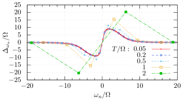
Figure 2: (Color online) Pairing of different Majorana fermions. Coupling strength is set to $g=6\Omega$. The gap function peaks at the larger of the two energy scales, temperature $\pi T$ or boson frequency $\Omega$.

Critical coupling and effective Schrödinger equation

The $T\ll\Omega$ analysis above indicates the possibility of a critical coupling $g_{c}\sim\Omega$ at zero temperature. This agrees with our numerically determined phase diagram Fig. 3. To clarify this question, we now analyze the gap equation at $T=0$ and $\Delta\rightarrow 0$, which may then be linearized and transformed into a differential equation in time

$$\left[-\frac{d^{2}}{dx^{2}}-V(x)\right]Y(x)=0\ ,$$ (21)

where $x=\tau^{\prime}-\tau$, $Y(x)=-Y(-x)$ is the Fourier transform of $\Delta^{-}_{\omega}/\omega^{2}$, and $V(x)=g^{2}e^{-\Omega|x|}$. This is a “Schrödinger equation” for energy eigenvalue $E=0$. The condition for the lowest-lying odd-parity state to have energy $E=0^{-}$ is found as

$$g_{c}(T=0)=\frac{\pi}{\gamma}\Omega\ ,$$ (22)

where $\gamma=2$ if $V(x)$ is approximated by a square well of depth $g^{2}$ and width $\Omega^{-1}$, in which case $Y(x)\propto\sin(g_{c}x)$ inside the potential well and decays rapidly on the outside, hence $\Delta_{\omega_{n}}^{-}$ peaks at $\omega_{\textsf{peak}}=g_{c}$. Numerically we found $\gamma\simeq 2.6$, see Fig. 3. We have a quantum critical point at $g=g_{c}$ separating the normal phase from the paired phase.

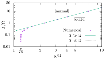
Figure 3: (Color online) Phase diagram in log scale at $\Omega=1$. Colored crosses: numerical results for the phase boundary $T_{c}(g)$. Green solid line: high $T$ limit Eq. 19. Gray dashed line: $T\rightarrow 0$ limit Eq. 22.

Ginzburg-Landau theory

In order to understand the interplay of odd-f and even-f pairing better we now formulate a Ginzburg-Landau free energy expression. As a suitable order parameter for odd-f pairing we choose the slope $A$ of the frequency dependent gap function, $\Delta^{-}=A\omega$ in the low frequency regime $|\omega_{n}|<\omega_{x}$. The even-f order parameter we define as $B=\Delta^{+}/\Omega$. Then, the free energy of low frequency modes as derived from Eq.14 may be approximated as (see SM)

$$F=c_{0}\Bigl{[}\left(t-1\right)A^{2}+\frac{A^{4}}{8}\Bigr{]}+\Bigl{[}\left(b_{0}t+4c_{1}\right)B^{2}+2c_{2}B^{4}\Bigr{]}-c_{1}A^{2}B^{2}$$ (23)

where $t\equiv\frac{T}{T_{c}}$, $b_{\ell}=T_{c}\sum_{m,n}^{\prime}\frac{(\omega_{m}\omega_{n})^{\ell}}{16g^{2}\Omega^{2(\ell-1)}}[K^{-1}]_{mn}$, $c_{\ell}=\frac{1}{4}\sum_{n}^{\prime}[\frac{\Omega}{2\omega_{n}}]^{2\ell}$ and $\sum^{\prime}$ is restricted to $|\omega_{n}|<\omega_{x}$, with $\omega_{x}$ chosen such that $b_{1}=c_{0}$. It is seen that as found numerically odd-f pairing appears for $T<T_{c}$ (provided $g>g_{c}$), whereas even-f pairing always increases the free energy, even taking into account the negative contribution of the mixed term (for details, see SM).

Conclusion

We extended Berezinskii’s classification of pairing order parameters to Majorana fermions, and showed that odd frequency pairing arises naturally in both free and interacting Majorana theories. For free Majoranas, odd-f pairing is the only pairing channel allowed by the fermionic exchange statistics. With interaction, pairing of Majorana fermions at opposite ends of a topological wire may be induced. We show that within a model of phonon-mediated interaction there is a critical coupling strength for pairing, which implies the existence of a quantum critical point, and can be determined by mapping the gap equation onto an effective Schrödinger equation. We find possible pairing solutions both analytically and numerically and show that only odd-f pairing is stable, although even-f pairing is in principle allowed. To this end we define two frequency-independent order parameters characterizing both odd-f and even-f pairing and propose an effective Ginzburg-Landau free energy derived from the microscopic mean field action. The simple model study of Majorana pairing presented here opens the way for a study of more complex systems involving many Majorana states, e.g. located at opposite edges of a two-dimensional topological superconductor.

Note added

We recently became aware of a related work by Zhang and Nori Zhang and Nori (2015).

*

Appendix A Supplementary Material

In this note, we derive the gap equation in detail using both field theory and diagrammatic expansion. Then we discuss the free energy of the odd-f and even-f pairing fields.

Appendix B Field theoretic derivation of the gap equation

The Majorana action from the text is

$$S=S_{0}+S_{\textsf{int}}\quad,\quad S_{0}=\int d\tau(\mu\partial_{\tau}\mu+\eta\partial_{\tau}\eta)\quad,\quad S_{\textsf{int}}=-8g^{2}\int\limits_{\mathclap{\tau<\tau^{\prime}}}d\tau d\tau^{\prime}K_{\tau,\tau^{\prime}}\mu_{\tau}\mu_{\tau^{\prime}}\eta_{\tau}\eta_{\tau^{\prime}}\ ,$$ (1)

$$K_{\tau,\tau^{\prime}}=\frac{1}{2}\left[e^{-\Omega|\tau^{\prime}-\tau|}+\frac{2\cosh\left[\Omega(\tau^{\prime}-\tau)\right]}{e^{\beta\Omega}-1}\right]\quad,\quad K_{\nu_{n}}=\frac{\Omega}{\Omega^{2}+\nu_{n}^{2}}\ .$$ (2)

Since $K_{\tau,\tau^{\prime}}=K_{\tau^{\prime},\tau}$, the $\tau>\tau^{\prime}$ interaction is equivalent to that of $\tau<\tau^{\prime}$ and is accounted for by doubling the prefactor in $S_{\textsf{int}}$. The purpose of keeping track of such redundancy in the interacting action is to avoid introducing multiple Hubbard-Stratonovich (HS) fields for equivalent interaction terms.

HS transformation uses the following identity: for a real positive number $M$ and any four Grassmann variables $\psi_{1},\psi_{2},\psi_{3},\psi_{4}$,

$$e^{M\psi_{1}\psi_{2}\psi_{3}\psi_{4}}=e^{M\psi_{1}\psi_{2}\psi_{3}\psi_{4}}\times\left[\int d\hat{\Delta}d\hat{\Delta}^{*}\,e^{-(\hat{\Delta}^{*}-M\psi_{1}\psi_{2})M^{-1}(\hat{\Delta}-M\psi_{3}\psi_{4})}\right]=\int d\hat{\Delta}d\hat{\Delta}^{*}\exp\left[-\frac{|\hat{\Delta}|^{2}}{M}+\hat{\Delta}\psi_{1}\psi_{2}+\hat{\Delta}^{*}\psi_{3}\psi_{4}\right]\ ,$$ (3)

upon proper normalization of the integration measure $d\hat{\Delta}d\hat{\Delta}^{*}$. To decouple $S_{\textsf{int}}$ in the $\mu\eta$ pairing channel, we use Eq. 3 and introduce, for each pair of time indices $\tau,\tau^{\prime}$ with $\tau<\tau^{\prime}$, a complex field $\hat{\Delta}_{\tau,\tau^{\prime}}$. After HS transformation, $S_{\textsf{int}}$ becomes

$$S_{\textsf{int}}^{\textsf{HS}}=\int\limits_{\mathclap{\tau<\tau^{\prime}}}d\tau d\tau^{\prime}\,\left[\frac{\left|\hat{\Delta}_{\tau,\tau^{\prime}}\right|^{2}}{8g^{2}K_{\tau,\tau^{\prime}}}-\hat{\Delta}_{\tau,\tau^{\prime}}\mu_{\tau}\eta_{\tau^{\prime}}-\hat{\Delta}^{*}_{\tau,\tau^{\prime}}\mu_{\tau^{\prime}}\eta_{\tau}\right]\ .$$ (4)

Note that $\hat{\Delta}$ is only defined for $\tau<\tau^{\prime}$. One can introduce a new field $\Delta_{\tau,\tau^{\prime}}$ with unrestricted time indices,

$$\Delta_{\tau,\tau^{\prime}}=\begin{cases}\hat{\Delta}_{\tau,\tau^{\prime}}&\tau<\tau^{\prime}\\ \hat{\Delta}^{*}_{\tau^{\prime},\tau}&\tau>\tau^{\prime}\end{cases}\ .$$ (5)

If $\Delta_{\tau,\tau^{\prime}}$ only depends on the time difference $\tau^{\prime}-\tau$, then Eq. 5 entails that the Fourier transform of $\Delta(\tau^{\prime}-\tau)$ is real,

$$\Delta_{\omega_{n}}=\int d\tau\Delta(\tau)e^{i\omega_{n}\tau}=\int\limits_{\tau>0}d\tau\left(\Delta(\tau)e^{i\omega_{n}\tau}+\text{c.c.}\right)\in\mathbb{R}\ .$$ (6)

Using the $\Delta$ fields, Eq. 4 can be rewritten as

$$S_{\textsf{int}}^{\textsf{HS}}=\int d\tau d\tau^{\prime}\left[\frac{\Delta_{\tau,\tau^{\prime}}\Delta_{\tau^{\prime},\tau}}{16g^{2}K_{\tau,\tau^{\prime}}}-\Delta_{\tau,\tau^{\prime}}\mu_{\tau}\eta_{\tau^{\prime}}\right]\ .$$ (7)

Reinstating $S_{0}$ and going to frequency domain, the full action is

$$S^{\textsf{HS}}=\sum_{\omega_{m},\omega_{n}}\frac{\Delta_{\omega_{m}}\Delta_{\omega_{n}}}{16g^{2}\beta}\left[\frac{1}{K}\right]_{\omega_{n}-\omega_{m}}+\underbrace{\sum_{\omega_{n}>0}(\mu_{\omega_{n}}\ ,\ \eta_{\omega_{n}})\overbrace{\begin{pmatrix}2i\omega_{n}&-\Delta_{\omega_{n}}\\ \Delta_{-\omega_{n}}&2i\omega_{n}\end{pmatrix}}^{\equiv\hat{G}_{\omega_{n}}^{-1}}\begin{pmatrix}\mu_{-\omega_{n}}\\ \eta_{-\omega_{n}}\end{pmatrix}}_{\equiv S_{\textsf{Fer}}}\ .$$ (8)

The fermion part is bilinear and can be integrated out,

$$Z_{\textsf{Fer}}=\int D(\bar{\psi},\psi)e^{-S_{\textsf{Fer}}}=\prod_{\omega_{n}>0}\left[-\frac{1}{4}\textsf{Det}\hat{G}_{\omega_{n}}^{-1}\right]=\prod_{\omega_{n}>0}(\omega_{n}^{2}-\frac{1}{4}\Delta_{\omega_{n}}\Delta_{-\omega_{n}})\ ,$$ (9)

where the factor $-1/4$ comes from the Jacobian $\partial(\mu_{\omega},\mu_{-\omega},\eta_{\omega},\eta_{-\omega})/\partial(\bar{\psi}_{\omega},\psi_{\omega},\bar{\psi}_{-\omega},\psi_{-\omega})$. The effective action of $\Delta$ thus reads

$$S_{\textsf{Eff}}=\sum_{\mathclap{\omega_{m},\omega_{n}}}\frac{\Delta_{\omega_{m}}\Delta_{\omega_{n}}}{16g^{2}\beta}\left[\frac{1}{K}\right]_{\omega_{m}-\omega_{n}}\mathclap{-}\sum_{\omega_{n}>0}\log\left(\omega_{n}^{2}-\frac{1}{4}\Delta_{\omega_{n}}\Delta_{-\omega_{n}}\right)\ ,$$ (10)

and minimization with respect to $\Delta$ yields the gap equation

$$\frac{1}{2g^{2}\beta}\sum_{\omega_{m}}\left[\frac{1}{K}\right]_{\quad\ \mathclap{\omega_{n}-\omega_{m}}}\Delta_{\omega_{m}}=\frac{\Delta_{-\omega_{n}}}{\frac{1}{4}\Delta_{\omega_{n}}\Delta_{-\omega_{n}}-\omega_{n}^{2}}\ .$$ (11)

Appendix C Gap equation from diagrammatic expansion

In this section, we treat the interacting action $S_{\textsf{int}}$ (Eq. 1) as a perturbation, and derive the gap equation as the one-loop correction to the self energy. We will use $\nu$ and $\omega$ to denote bosonic and fermionic Matsubara frequencies, respectively.

Let us introduce two-component Grassmann vectors,

$$\Psi_{\omega}=\begin{pmatrix}\mu_{\omega}\\ \eta_{\omega}\end{pmatrix}\quad,\quad\bar{\Psi}_{\omega}=(\mu_{-\omega}\ ,\ \eta_{-\omega})\ .$$ (12)

The matrix Green’s function is defined as

$$\hat{G}_{\omega}\equiv\langle\Psi_{\omega}\bar{\Psi}_{\omega}\rangle=\Bigl{<}\begin{pmatrix}\mu_{\omega}\mu_{-\omega}&\mu_{\omega}\eta_{-\omega}\\ \eta_{\omega}\mu_{-\omega}&\eta_{\omega}\eta_{-\omega}\end{pmatrix}\Bigr{>}\ .$$ (13)

It is equivalent to the Majorana pairing matrix $M$ defined in the text. One has

$$\hat{G}_{\omega}^{\alpha\beta}=\frac{\langle\Psi_{\omega}^{\alpha}\bar{\Psi}_{\omega}^{\beta}e^{-S_{\textsf{int}}}\rangle_{0}}{\langle e^{-S_{\textsf{int}}}\rangle_{0}}$$ (14)

where $\langle\cdots\rangle_{0}$ denotes averaging over the free action $S_{0}$, and in the vector notation, the interacting action can be written as

$$-S_{\textsf{int}} =g^{2}\int d\tau d\tau^{\prime}K_{\tau\tau^{\prime}}\left[\bar{\Psi}_{\tau}\hat{\lambda}\Psi_{\tau}\right]\left[\bar{\Psi}_{\tau^{\prime}}\hat{\lambda}\Psi_{\tau^{\prime}}\right]$$ (15)

$$=g^{2}T\sum_{\nu,\omega_{1,2,3,4}}K_{\nu}\left[\bar{\Psi}_{\omega_{1}}\hat{\lambda}\Psi_{\omega_{2}}\right]\left[\bar{\Psi}_{\omega_{3}}\hat{\lambda}\Psi_{\omega_{4}}\right]\delta(\omega_{1}-\omega_{2}-\nu)\delta(\omega_{3}-\omega_{4}+\nu)\ ,$$ (16)

where the matrix $\hat{\lambda}=-\sigma_{y}$. The summand corresponds to the diagram Fig. 4a. To the order of $g^{2}$, Eq. 14 becomes

$$\hat{G}_{\omega}^{\alpha\beta}=\frac{\langle\Psi_{\omega}^{\alpha}\bar{\Psi}_{\omega}^{\beta}(1-S_{\textsf{int}})\rangle_{0}}{1-\langle S_{\textsf{int}}\rangle_{0}}=\langle\Psi_{\omega}^{\alpha}\bar{\Psi}_{\omega}^{\beta}\rangle_{0}+\langle\Psi_{\omega}^{\alpha}\bar{\Psi}_{\omega}^{\beta}\times(-S_{\textsf{int}})\rangle_{0}^{c}+\mathcal{O}(g^{4})\ ,$$ (17)

where the superscript $c$ denotes connected contractions, i.e. both $\Psi_{\omega}^{\alpha}$ and $\bar{\Psi}_{\omega}^{\beta}$ are to be contracted with fields in $S_{\textsf{int}}$, not with each other. Explicitly written out, one has (summing over repeated indices)

$$\langle\Psi_{\omega}^{\alpha}\bar{\Psi}_{\omega}^{\beta}\times(-S_{\textsf{int}})\rangle_{0}^{c}=g^{2}T\sum_{\nu,\omega_{1,2,3,4}}K_{\nu}\delta(\omega_{1}-\omega_{2}-\nu)\delta(\omega_{3}-\omega_{4}+\nu)\hat{\lambda}^{ab}\hat{\lambda}^{cd}\times\langle\Psi_{\omega}^{\alpha}\times\bar{\Psi}_{\omega_{1}}^{a}\Psi_{\omega_{2}}^{b}\bar{\Psi}_{\omega_{3}}^{c}\Psi_{\omega_{4}}^{d}\times\bar{\Psi}_{\omega}^{\beta}\rangle_{0}^{c}\ .$$ (18)

If we ignore the Hartree terms in $\langle\cdots\rangle_{0}^{c}$, i.e., those with the two external fields $\Psi^{\alpha}$ and $\bar{\Psi}^{\beta}$ contracting on the same $\hat{\lambda}$ vertex, then it corresponds to the diagram Fig. 4b, and since there is no distinction between particle and hole for Majorana fermions, $\Psi^{\alpha}$ can contract with any of $a,b,c,d$, and $\bar{\Psi}^{\beta}$ can then contract with two of $a,b,c,d$ on the opposite vertex of $\Psi^{\alpha}$. There are $4\times 2$ such contractions of identical results. For example, consider the contraction of $\langle\alpha,b\rangle\langle a,c\rangle\langle d,\beta\rangle$. The two “anomalous” ones are

$$\langle\Psi^{\alpha}_{\omega}\Psi^{b}_{\omega_{2}}\rangle_{0}=\delta_{\omega,-\omega_{2}}G_{\omega}^{(0)\alpha b}\quad,\quad\langle\bar{\Psi}_{\omega_{1}}^{a}\bar{\Psi}^{c}_{\omega_{3}}\rangle_{0}=\delta_{\omega_{1},-\omega_{3}}G_{-\omega_{1}}^{(0)ac}\ .$$ (19)

From the delta functions one has $\omega_{4}=-\omega_{2}=\omega$ and $\omega_{3}=-\omega_{1}=\omega-\nu$. The contribution to the RHS of Eq. 18 is thus

$$-g^{2}T\sum_{\nu}K_{\nu}\hat{\lambda}^{ab}\hat{\lambda}^{cd}\times\hat{G}_{\omega}^{(0)\alpha b}\hat{G}_{\omega-\nu}^{(0)ac}\hat{G}_{\omega}^{(0)d\beta}=g^{2}T\left[\hat{G}_{\omega}^{(0)}\hat{\lambda}\left(\sum_{\nu}K_{\nu}\hat{G}^{(0)}_{\omega-\nu}\right)\hat{\lambda}\hat{G}_{\omega}^{(0)}\right]^{\alpha\beta}\ ,$$ (20)

where the minus sign comes from exchanging the order of $a$ and $b$ in the contraction, and we used $-\hat{\lambda}^{T}=\hat{\lambda}$. Eq. 18 is then

$$\langle\Psi_{\omega}^{\alpha}\bar{\Psi}_{\omega}^{\beta}\times(-S_{\textsf{int}})\rangle_{0}^{c}=\left[\hat{G}_{\omega}^{(0)}\hat{\Sigma}_{\omega}\hat{G}_{\omega}^{(0)}\right]^{\alpha\beta}$$ (21)

where

$$\hat{\Sigma}_{\omega}=8\times g^{2}T\sum_{\nu}K_{\nu}\left[\hat{\lambda}\hat{G}_{\omega-\nu}^{(0)}\hat{\lambda}\right]\ .$$ (22)

Comparing Eq. 17 with the definition of self energy,

$$\Sigma_{\omega}\equiv(G^{(0)}_{\omega})^{-1}-G_{\omega}^{-1}\Leftrightarrow G_{\omega}=G_{\omega}^{(0)}+G_{\omega}^{(0)}\Sigma_{\omega}G_{\omega}^{(0)}+G_{\omega}^{(0)}\Sigma_{\omega}G_{\omega}^{(0)}\Sigma_{\omega}G_{\omega}^{(0)}+\cdots\ ,$$ (23)

one can identify that up to leading correction, Eq. 22 is indeed the self energy. Replacing $\hat{G}^{(0)}$ with the full $\hat{G}$ on the RHS of Eq. 22 then leads to the self consistent equation for the self energy matrix,

$$\hat{\Sigma}_{\omega}=8\times g^{2}T\sum_{\nu}K_{\nu}\left[\hat{\lambda}\hat{G}_{\omega-\nu}\hat{\lambda}\right]\ .$$ (24)

Now writing

$$\hat{G}_{\omega}^{-1}\equiv\begin{pmatrix}2i\omega&-\Delta_{\omega}\\ \Delta_{-\omega}&2i\omega\end{pmatrix}\implies\hat{G}_{\omega}=\frac{\begin{pmatrix}2i\omega&\Delta_{\omega}\\ -\Delta_{-\omega}&2i\omega\end{pmatrix}}{\textsf{Det}\hat{G}^{-1}_{\omega}}\implies\hat{\lambda}\hat{G}_{\omega}\hat{\lambda}=\frac{\begin{pmatrix}2i\omega&\Delta_{-\omega}\\ -\Delta_{\omega}&2i\omega\end{pmatrix}}{\textsf{Det}\hat{G}_{\omega}^{-1}}\ ,$$ (25)

note that $\hat{G}^{-1}$ is the same fermion kernel as one would get in the field theoretic approach, cf. Eq. 8. Then the self consistent equation for the matrix element $\hat{\Sigma}_{\omega}^{12}$ reads

$$\Delta_{\omega}=8g^{2}T\sum_{\omega^{\prime}}K_{\omega-\omega^{\prime}}\frac{\Delta_{-\omega^{\prime}}}{\Delta_{\omega^{\prime}}\Delta_{-\omega^{\prime}}-4{\omega^{\prime}}^{2}}\ ,$$ (26)

which is the same as Eq. 11 obtained from minimizing the HS action. Eqs. 11 and 26 appear to have different factors of $T$, this is due to the convention of the Fourier transform $A_{\nu}=\int d\tau A_{\tau}e^{i\nu\tau}$, and the fact that $K_{\tau}$ is dimensionless, thus both $K_{\nu}$ and $(1/K)_{\nu}$ have a dimension of time, hence the different factors of $T$.

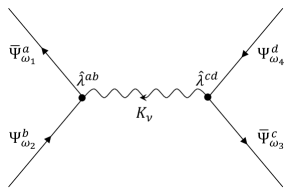
(a)

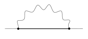
(b)

Figure 4: Feynman diagrams. (a): Interaction vertex, see Eq. 16. Frequencies going into the same $\hat{\lambda}$ vertex sum to zero, and arrows denote the sign of the corresponding frequency in the $\delta$ function. (b): Self energy at the one loop level, see discussion below Eq. 18 for multiplicity. Thick line represents the dressed Green’s function used in the self consistent equation Eq. 24.

Appendix D Free energy consideration of the odd-f and even-f pairing states

Consider the action Eq. 10 relative to the normal state $\Delta=0$ (which is always a solution of the gap equation),

$$\delta S(\Delta)\equiv S_{\textsf{Eff}}(\Delta)-S_{\textsf{Eff}}(0)=\sum_{\mathclap{\omega_{m},\omega_{n}}}\frac{\Delta_{\omega_{m}}\Delta_{\omega_{n}}}{16g^{2}\beta}\left[\frac{1}{K}\right]_{\omega_{m}-\omega_{n}}\mathclap{-}\sum_{\omega_{n}>0}\log\left(1-\frac{\Delta_{\omega_{n}}\Delta_{-\omega_{n}}}{4\omega_{n}^{2}}\right)\ .$$ (27)

For any even-f configuration $\Delta_{-\omega_{n}}=\Delta_{\omega_{n}}$, $\delta S(\Delta)\geq 0$, because the first term is positive definite, and in the second term, $\log(1-\Delta_{\omega_{n}}^{2}/4\omega_{n}^{2})<0$. Thus without solving the gap equation, one can already conclude that any even-f state will be unstable.

In the diagonal limit $K_{\nu_{n}}=\delta_{\nu_{n},0}K_{0}$, the odd-f solution to Eq. 26 is

$$\Delta_{\omega_{n}}^{-}=-\Delta_{-\omega_{n}}^{-}=2\sqrt{g^{2}TK_{0}-\omega_{n}^{2}}\ .$$ (28)

From Eq. 27, the action contributed by $\Delta_{\omega_{n}}$ and $\Delta_{-\omega_{n}}$ is

$$\delta S_{\omega_{n}}=1-\frac{\omega_{n}^{2}}{2g^{2}TK_{0}}-\log\frac{2g^{2}TK_{0}}{\omega_{n}^{2}}\ .$$ (29)

One can verify that $1-x+\log x\leq 0$, with equality occuring at $x=1$, thus the odd-f solution Eq. 28 has a lower free energy than the normal state and is stable.

To understand in a more general way why only the odd-f state is stable, one may adopt the Ginzburg-Landau perspective and expand the $\log$ term in Eq. 27 to quartic order in $\Delta$, keeping both, odd-f and even-f components, $\Delta^{\pm}_{\omega_{n}}=\frac{1}{2}(\Delta_{\omega_{n}}\pm\Delta_{-\omega_{n}})$,

$$\delta S(\Delta)=\sum_{\mathclap{\omega_{m},\omega_{n}}}\frac{\Delta^{-}_{\omega_{m}}\Delta^{-}_{\omega_{n}}+\Delta^{+}_{\omega_{m}}\Delta^{+}_{\omega_{n}}}{16g^{2}\beta}\left[\frac{1}{K}\right]_{\omega_{m}-\omega_{n}}+\sum_{\omega_{n}>0}\left[\frac{(\Delta^{+}_{\omega_{n}})^{2}-(\Delta^{-}_{\omega_{n}})^{2}}{4\omega_{n}^{2}}+\frac{(\Delta^{+}_{\omega_{n}})^{4}+(\Delta^{-}_{\omega_{n}})^{4}-2(\Delta^{+}_{\omega_{n}})^{2}(\Delta^{-}_{\omega_{n}})^{2}}{32\omega_{n}^{\,4}}\right]+\mathcal{O}(\Delta^{6})\ .$$ (30)

The first term on the r.h.s. does not have a mixed term owing to the even symmetry of $1/K$. We now immediately see that the odd-f component contributes a negative contribution in quadratic order, which may induce a transition, while the even-f contribution does not. However, while the fourth order terms of both pure odd-f and pure even-f type are positive, the mixed term is negative. This opens the possibility that in an odd-f paired state, even-f pairing may be induced at some lower temperature. In order to explore this scenario we first simplify the analysis by defining frequency independent dimensionless order parameters $A,B$ , where $A$ is the initial slope of $\Delta^{-}$, $\Delta^{-}_{\omega_{n}}=A\omega_{n}$ and $B=\Delta^{+}_{\omega_{n}}/\Omega$ . We restrict the frequency integrations to low frequency, $|\omega_{n}|<\omega_{x}$, where the cutoff $\omega_{x}$ is to be suitably defined later. The above action may then be expressed as a Ginzburg-Landau free energy expansion in the order parameters $A,B$,

$$F(A,B)\equiv\delta S(\Delta)=c_{0}\left[\left(t-1\right)A^{2}+\frac{A^{4}}{8}\right]+\Bigl{[}\left(b_{0}t+4c_{1}\right)B^{2}+2c_{2}B^{4}\Bigr{]}-c_{1}A^{2}B^{2}+\mathcal{O}(A^{6},B^{6},\cdots)\ .$$ (31)

Here we defined $t=\frac{T}{T_{c}}$ and the positive dimensionless coefficients

$$b_{\ell}=T_{c}\sideset{}{{}^{\prime}}{\sum}_{\omega_{m},\omega_{n}}\frac{(\omega_{m}\omega_{n})^{\ell}}{16g^{2}\Omega^{2(\ell-1)}}\left[\frac{1}{K}\right]_{\omega_{m}-\omega_{n}}\quad,\quad c_{\ell}=\frac{1}{4}\sideset{}{{}^{\prime}}{\sum}_{\omega_{n}>0}\left[\frac{\Omega}{2\omega_{n}}\right]^{2\ell}\ ,$$ (32)

the primed sum imposes the aforementioned frequency cutoff $\omega_{x}$ implicitly determined by requiring

$$b_{1}\stackrel{{\scriptstyle!}}{{=}}c_{0}\ .$$ (33)

If we now substitute the meanfield solution $A^{2}=4(1-T/T_{c})$ for odd-f pairing (assuming $g>g_{c}$) into the mixed term we find that the determining equation for $B$,

$$\frac{\partial F}{\partial(B^{2})}=(b_{0}+4c_{1})t+4c_{2}B^{2}\stackrel{{\scriptstyle!}}{{=}}0\ ,$$ (34)

does not have a real solution for any positive $t$.

References

- Kitaev (2001) A. Y. Kitaev, Physics-Uspekhi 44, 131 (2001).
- Alicea (2012) J. Alicea, Reports on Progress in Physics 75, 076501 (2012).
- Cheng et al. (2010) M. Cheng, R. M. Lutchyn, V. Galitski, and S. Das Sarma, Phys. Rev. B 82, 094504 (2010).
- Rokhinson et al. (2012) L. P. Rokhinson, X. Liu, and J. K. Furdyna, Nature Physics 8, 795 (2012).
- Wilczek (2009) F. Wilczek, Nature Physics 5, 614 (2009).
- Mourik et al. (2012) V. Mourik, K. Zuo, S. M. Frolov, S. R. Plissard, E. P. A. M. Bakkers, and L. P. Kouwenhoven, Science 336, 1003 (2012).
- Churchill et al. (2013) H. O. H. Churchill, V. Fatemi, K. Grove-Rasmussen, M. T. Deng, P. Caroff, H. Q. Xu, and C. M. Marcus, Phys. Rev. B 87, 241401 (2013).
- Wang et al. (2014) D. Wang, Z. Huang, and C. Wu, Phys. Rev. B 89, 174510 (2014).
- Kitaev (2003) A. Kitaev, Annals of Physics 303, 2 (2003), ISSN 0003-4916.
- Nayak et al. (2008) C. Nayak, S. H. Simon, A. Stern, M. Freedman, and S. Das Sarma, Rev. Mod. Phys. 80, 1083 (2008).
- Beenakker (2013) C. Beenakker, Annual Review of Condensed Matter Physics 4, 113 (2013).
- Asano and Tanaka (2013) Y. Asano and Y. Tanaka, Phys. Rev. B 87, 104513 (2013).
- Liu et al. (2015) X. Liu, J. D. Sau, and S. Das Sarma, Phys. Rev. B 92, 014513 (2015).
- Berezinskii (1974) V. Berezinskii, JETP Lett 20, 287 (1974).
- Balatsky and Abrahams (1992) A. Balatsky and E. Abrahams, Phys. Rev. B 45, 13125 (1992).
- Belitz and Kirkpatrick (1992) D. Belitz and T. R. Kirkpatrick, Phys. Rev. B 46, 8393 (1992).
- Abrahams et al. (1995) E. Abrahams, A. Balatsky, D. J. Scalapino, and J. R. Schrieffer, Phys. Rev. B 52, 1271 (1995).
- Bergeret et al. (2005) F. S. Bergeret, A. F. Volkov, and K. B. Efetov, Rev. Mod. Phys. 77, 1321 (2005).
- Tanaka et al. (2012) Y. Tanaka, M. Sato, and N. Nagaosa, Journal of the Physical Society of Japan 81, 011013 (2012).
- Burset et al. (2015) P. Burset, B. Lu, G. Tkachov, Y. Tanaka, E. M. Hankiewicz, and B. Trauzettel, ArXiv e-prints (2015), eprint 1508.07173.
- Ebisu et al. (2015) H. Ebisu, B. Lu, K. Taguchi, A. A. Golubov, and Y. Tanaka, ArXiv e-prints (2015), eprint 1509.01914.
- Black-Schaffer et al. (2013) A. M. Black-Schaffer et al., Phys. Rev. B 87, 220506 (2013).
- Black-Schaffer and Balatsky (2013) A. M. Black-Schaffer and A. V. Balatsky, Phys. Rev. B 88, 104514 (2013).
- Balatsky and Abrahams (1995) A. V. Balatsky and E. Abrahams, Phys. Rev. Lett. 74, 1004 (1995).
- Balatsky (2014) A. V. Balatsky, ArXiv e-prints (2014), eprint 1409.4875.
- Kedem and Balatsky (2015) Y. Kedem and A. V. Balatsky, ArXiv e-prints (2015), eprint 1501.07049.
- Chiu et al. (2014) C.-K. Chiu, D. I. Pikulin, and M. Franz, ArXiv e-prints (2014), eprint 1411.5802.
- Katsura et al. (2015) H. Katsura, D. Schuricht, and M. Takahashi, ArXiv e-prints (2015), eprint 1507.04444.
- Note (1) Note1, can be understood as the statistical weight of the Majorana pair .
- Solenov et al. (2009) D. Solenov, I. Martin, and D. Mozyrsky, Phys. Rev. B 79, 132502 (2009).
- Zhang and Nori (2015) P. Zhang and F. Nori, Phys. Rev. B 92, 115303 (2015).
*