Phenomenological description of the nonlocal magnetization relaxation in magnonics, spintronics, and domain-wall dynamics

Abstract

A phenomenological equation called Landau-Lifshitz-Baryakhtar (LLBar) equation, which could be viewed as the combination of Landau-Lifshitz (LL) equation and an extra “exchange damping” term, was derived by Baryakhtar using Onsager’s relations. We interpret the origin of this “exchange damping” as nonlocal damping by linking it to the spin current pumping. The LLBar equation is investigated numerically and analytically for the spin wave decay and domain wall motion. Our results show that the lifetime and propagation length of short-wavelength magnons in the presence of nonlocal damping could be much smaller than those given by LL equation. Furthermore, we find that both the domain wall mobility and the Walker breakdown field are strongly influenced by the nonlocal damping.

I Introduction

The genuine complexity of magnetic and spintronic phenomena occurring in magnetic samples and devices imposes both fundamental and technical limits on the applicability of quantum-mechanical and atomistic theories to their modeling. To a certain degree, this challenge can be circumvented by exploiting phenomenological theories based on the continuous medium approximation. The theories operate with the magnetization (i.e. the magnetic moment density) and the effective magnetic field as generalized coordinates and forces respectively Landau and Lifshitz (1935); Akhiezer et al. (1968). The effective magnetic field is defined in terms of various magnetic material parameters, which are determined by fitting theoretical results to experimental data, and at least in principle, can be calculated using the quantum-mechanical or atomistic methods. However, solving the phenomenological models analytically is still a formidable task in the majority of practically important cases. The difficulty is primarily due to the presence of the long range magneto-dipole interaction and associated non-uniformity of the ground state configurations of both the magnetization and effective magnetic field. Hence, the phenomenological models are solved instead numerically, using either finite-difference or finite-element methods realized in a number of micromagnetic solvers Donahue and Porter (1999); Scholz et al. (2003); Fischbacher et al. (2007); Berkov and Gorn (2008); Vansteenkiste et al. (2014).

Traditionally, the software for such numerical micromagnetic simulations of magnetization dynamics is based on solving the Landau-Lifshitz equation Landau and Lifshitz (1935) with a transverse magnetic relaxation term, either in the original (Landau) Landau and Lifshitz (1935) or ”Gilbert” Gilbert (2004) form. Over time, dictated by the experimental and technological needs, the solvers have been modified to include finite temperature effects García-Palacios and Lázaro (1998) and additional contributions to the magnetic energy (and therefore to effective magnetic field) Shu et al. (2004). The recent advances in spintronics and magnonics have led to the implementation of various spin transfer torque terms Zhang and Li (2004); Thiaville et al. (2005) and periodic boundary conditions Lebecki et al. (2008); Wang et al. (2010); Krueger and Selke (2013). Furthermore, the progress in experimental investigations of ultrafast magnetization dynamics Kirilyuk et al. (2010) has exposed the need to account for the variation of the length of the magnetization vector in response to excitation by femtosecond optical pulses, leading to inclusion of the longitudinal relaxation of the magnetization within the formalism of numerical micromagnetics Au et al. (2013). Provided that a good agreement between the simulated and measured results is achieved, a microscopic (i.e. quantum-mechanical or atomistic) interpretation of the experiments can then be developed.

The described strategy relies on the functional completeness of the phenomenological model. For instance, a forceful use of incomplete equations to describe phenomena originating from terms missing from the model may result in false predictions and erroneous values of fitted parameters, and eventually in incorrect conclusions. The nature of the magnetic relaxation term and associated damping constants in the Landau-Lifshitz equation is of paramount importance both fundamentally and technically. It is this term that is responsible for establishment of equilibrium both within the magnetic sub-system and with its environment (e.g. electron and phonon sub-systems), following perturbation by magnetic fields, spin currents, and/or optical pulses Kirilyuk et al. (2010). Moreover, it is the same term that will eventually determine the energy efficiency of any emerging nano-magnetic devices, including both those for data storage Terris and Thomson (2005) and manipulation Kruglyak et al. (2010).

In this report, we demonstrate how the phenomenological magnetic relaxation term derived by Baryakhtar to explain the discrepancy between magnetic damping constants obtained from ferromagnetic resonance (FMR) and magnetic domain wall velocity measurements in dielectrics Baryakhtar (1998); Bar’yakhtar et al. (1986); Baryakhtar and Danilevich (2013) can be applied to magnetic metallic samples. We show that the Landau-Lifshitz equation with Baryakhtar relaxation term (Landau-Lifshitz-Baryakhtar or simply LLBar equation) contains the Landau-Lifshitz-Gilbert (LLG) equation as a special case, while also naturally including the contribution from the nonlocal damping in the tensor form of Zhang and Zhang Zhang and Zhang (2009) and De Angeli De Angeli et al. (2009). The effects of the longitudinal relaxation and the anisotropic transverse relaxation on the magnetization dynamics excited by optical and magnetic field pulses, respectively, in continuous films and magnetic elements were discussed e.g. in Ref. [17; 25; 26]. So, here we focus primarily on the manifestations of the Baryakhtar relaxation in problems specific for magnonics Kruglyak et al. (2010) and domain wall dynamics Hillebrands and Thiaville (2006); Weindler et al. (2014). This is achieved by incorporating the LLBar equation within the code of the Object Oriented Micromagnetic Framework (OOMMF) Donahue and Porter (1999), probably the most popular micromagnetic solver currently available, and by comparing the results of simulations with those from simple analytical models. Specifically, we demonstrate that the Baryakhtar relaxation leads to increased damping of short wavelength spin waves and to modification of the domain wall mobility, the latter being also affected by the longitudinal relaxation strength.

The paper is organized as follows. In Sec. II, we review and interpret the Baryakhtar relaxation term. In Sec. III, we calculate and analyze the spin wave decay in a thin magnetic nanowire. In Sec. IV, we simulate the the suppression of standing spin waves in thin film. In Sec. V, we analyze the domain wall motion driven by the external field and compare the relative strength of contributions from the longitudinal and nonlocal damping. We conclude the discussion in Sec. VI.

II Basic equations

In the most general case, the LLBar equation can be written as Baryakhtar (1998); Dvornik et al. (2013a)

$$\frac{\partial\mathbf{M}}{\partial t}=-\gamma\mathbf{M}\times\mathbf{H}_{\mathrm{eff}}+\mathbf{R}$$ (1)

where $\gamma(>0)$ is the gyromagnetic ratio and the relaxation term $\mathbf{R}$ is

$$\mathbf{R}=\hat{\Lambda}_{r}\cdot\mathbf{H}_{\mathrm{eff}}-\hat{\Lambda}_{e,sp}\frac{\partial^{2}{\mathbf{H}_{\mathrm{eff}}}}{\partial x_{s}\partial x_{p}}.$$ (2)

Here and in the rest of the paper, the summation is automatically assumed for repeated indices. The two relaxation tensors $\hat{\Lambda}_{r}$ and $\hat{\Lambda}_{e}$ describe relativistic and exchange contributions, respectively, as originally introduced in Ref. [21].

To facilitate comparison with the LLB equation as written in Ref. [29], the magnetic interaction energy of the sample is defined as

$$w=w_{\mu}+\frac{\mu_{0}}{8\chi}\frac{(M^{2}-M_{e}^{2})^{2}}{M_{e}^{2}},$$ (3)

where $M_{e}$ is the equilibrium magnitude of the magnetization vector at a given temperature and zero micromagnetic effective field, i.e. the effective field derived from the micromagnetic energy density $w_{\mu}$, as used in standard simulations at constant temperature under condition $|\mathbf{M}|=M_{e}=\mathrm{const}$ (i.e. with only the transverse relaxation included). The second term in right-hand side of Eq. (3) describes the energy density induced by the small deviations of the magnetization length from its equilibrium value $M_{e}$ at the given temperature, i.e., $|M^{2}-M_{e}^{2}|\ll M_{e}^{2}$, and $\chi$ is the longitudinal magnetic susceptibility. Therefore, the associated effective magnetic field is

$$\mathbf{H}_{\mathrm{eff}}=-\frac{1}{\mu_{0}}\frac{\delta w}{\delta\mathbf{M}}=\mathbf{H}_{\mu}+\frac{1}{2\chi}(1-n^{2})\mathbf{M}$$ (4)

where $\mathbf{n}=\mathbf{M}/M_{e}$, $\mathbf{H}_{\mu}$ is the effective magnetic field associated to $w_{\mu}$. Hereafter we assume that our system is in contact with the heat bath, so that the equilibrium temperature and associated value of $M_{e}$ and $\chi$ remain constant irrespective of the magnetization dynamics.

In accordance with the standard practice of both micromagnetic simulations and analytical calculations, to solve LLBar equations (1-4), one first needs to the corresponding static equations obtained by setting the time derivatives to zero and thereby to derive the spatial distribution of the magnetization in terms of both its length and direction. We note that, in general (e.g. as in the case of a domain wall), the resulting distribution of the longitudinal effective field and therefore also of the equilibrium magnetization length is nonuniform, so that the length is not generally equal to $M_{e}$. With the static solution at hands, the dynamical problem is solved so as to find the temporal evolution of the magnetization length and direction following some sort of a perturbation. Crudely speaking, the effect of the relaxation terms is that, at each moment of time, the magnetization direction relaxes towards the instantaneous direction of the effective magnetic field, while the magnetization length relaxes towards the value prescribed by the instantaneous longitudinal effective magnetic field. The effective field itself varies with time, which makes the problem rather complex. However, this is the same kind of complexity as the one that has always been inherent to micromagnetics. The account of the longitudinal susceptibility within the LLBar equation only brings another degree of freedom (the length of the magnetization) into the discussion. One should note however that the longitudinal susceptibility has a rather small value at low temperature and so its account is only required at temperatures of the order of the Curie temperature.

We neglect throughout the paper any effects due to the anisotropy of relaxation, which could be associated e.g. with the crystalline structure of the magnetic material Baryakhtar (1998); Dvornik et al. (2013a). This approximation is justified for polycrystalline and amorphous soft magnetic metals, as has been confirmed by simulations presented in Ref. [25]. Hence, we represent the relaxation tensors as $\hat{\Lambda}_{r}=\lambda_{r}\hat{I}$ and $\hat{\Lambda}_{e}=\lambda_{e}\hat{I}$ where parameters $\lambda_{r}$ and $\lambda_{e}$ are the relativistic and exchange relaxation damping constants and $\hat{I}$ is the unit tensor. Then, Eq. (1) is reduced to

$$\partial_{t}\mathbf{M}=-\gamma\mathbf{M}\times\mathbf{H}_{\mathrm{eff}}+\lambda_{r}\mathbf{H}_{\mathrm{eff}}-\lambda_{e}\nabla^{2}\mathbf{H}_{\mathrm{eff}}.$$ (5)

We separate the equations describing the dynamics and relaxation of the length and direction of the magnetization vector. Representing the latter as a product of its magnitude and directional unit vector $\mathbf{M}=M\mathbf{m}$, we can write

$$M\frac{\partial\mathbf{m}}{\partial t}+\mathbf{m}\frac{\partial M}{\partial t}=-\gamma\mathbf{M}\times\mathbf{H}_{\mathrm{eff}}+\mathbf{R}.$$ (6)

We multiply this equation by $\mathbf{m}$ to obtain,

$$\frac{\partial M}{\partial t}=\mathbf{m}\cdot\mathbf{R}.$$ (7)

Then, subtracting the product of equation (7) and $\mathbf{m}$ from equation (6), we obtain

$$\frac{\partial\mathbf{m}}{\partial t}=-\gamma\mathbf{m}\times\mathbf{H}_{\mathrm{eff}}+\frac{1}{M}\mathbf{R}_{\perp}$$ (8)

where $\mathbf{R}_{\perp}=-\mathbf{m}\times(\mathbf{m}\times\mathbf{R})$. In the rest of the paper, we will use $\mathbf{A}_{\perp}\equiv(\mathbf{A})_{\perp}\equiv\mathbf{A}-(\mathbf{A}\cdot\mathbf{m})\mathbf{m}$ to represent the component of the vector $\mathbf{A}$ that is perpendicular (transverse) to vector $\mathbf{m}$. Note that only the perpendicular component of the torque contributes to $\partial_{t}\mathbf{m}\equiv\partial{\mathbf{m}}/\partial t$. For given temperature, $M_{e}$ is constant and we can define $\alpha=\lambda_{r}/(\gamma M_{e})$. In the limiting case of $\chi\rightarrow 0$, $M\rightarrow M_{e}$ and thus $\alpha$ is recognized as the Gilbert damping constant from the LLG equation. Let us now consider the case of $\hat{\Lambda}_{e}\neq 0$. The corresponding contribution to the relaxation term, which we denote here as $\mathbf{B}_{\mathrm{Bar}}$, can be written as

$$\mathbf{B}_{\mathrm{Bar}}=-\lambda_{e}\nabla^{2}\mathbf{H}_{\mathrm{eff}}\equiv-\partial_{i}\mathbf{j}_{i},$$ (9)

where $\partial_{i}\equiv\partial/\partial x_{i}$ and the quantity $\mathbf{j}_{i}=-\lambda_{e}\partial_{i}\mathbf{H}_{\mathrm{eff}}$ has the form of some magnetization current density (magnetization flux).

For the following, it is useful to split the effective field into its perpendicular (relative to $\mathbf{m}$) part ($\mathbf{H}_{\mathrm{eff}}^{\perp}$, “perpendicular field”) and parallel part ($\mathbf{H}_{\mathrm{eff}}^{\parallel}$, “parallel field”), i.e., $\mathbf{H}_{\mathrm{eff}}=\mathbf{H}_{\mathrm{eff}}^{\perp}+\mathbf{H}_{\mathrm{eff}}^{\parallel}$, and then to consider the associated magnetic fluxes and torques separately. The magnetic flux of $\mathbf{j}_{\parallel,i}=-\lambda_{e}\partial_{i}\mathbf{H}_{\mathrm{eff}}^{\parallel}$ and then the contribution of the associated torque $\bm{\tau}_{\parallel}=-\partial_{i}\mathbf{j}_{\parallel,i}$ onto $\mathbf{m}$ is

$$(\bm{\tau}_{\parallel})_{\perp}=-2\lambda_{e}\partial_{i}\mathbf{H}_{\mathrm{eff}}^{\parallel}\partial_{i}\mathbf{m}-\lambda_{e}\mathbf{H}_{\mathrm{eff}}^{\parallel}(\nabla^{2}\mathbf{m})_{\perp}.$$ (10)

The perpendicular field can be represented as

$$\mathbf{H}_{\mathrm{eff}}^{\perp}=\frac{1}{\gamma M^{2}}\left[\mathbf{M}\times\frac{\partial\mathbf{M}}{\partial t}\right]+O(\mathbf{R})\approx\frac{1}{\gamma}\left[\mathbf{m}\times\partial_{t}\mathbf{m}\right].$$ (11)

So, we can write for the magnetization flux associated with the perpendicular field

$$\mathbf{j}_{\perp,i}=-(\lambda_{e}/\gamma)\partial_{i}(\mathbf{m}\times\partial_{t}\mathbf{m}).$$ (12)

The right-hand side of Eq. (12) could be regarded as the torque generated by spin current pumping since $\mathbf{m}\times\partial_{t}\mathbf{m}$ can be considered as the exchange spin current Tserkovnyak et al. (2009), and then for the associated perpendicular torque $\bm{\tau}_{\perp}$, we obtain,

$$\bm{\tau}_{\perp}=-\partial_{i}\mathbf{j}_{\perp,i}=-\sigma M_{e}\partial_{i}\partial_{i}(\mathbf{m}\times\partial_{t}\mathbf{m}),$$ (13)

where we have introduced variable $\sigma=\lambda_{e}/(\gamma M_{e})$. We show that the torque $(\bm{\tau}_{\perp})_{\perp}$ could be written as (see Appendix A for details)

$$(\bm{\tau}_{\perp})_{\perp}=M_{e}\left[\mathbf{m}\times(\mathcal{D}\cdot\partial_{t}\mathbf{m})-\sigma\mathbf{m}\times\nabla^{2}\partial_{t}\mathbf{m}\right]$$ (14)

where $\mathcal{D}$ is a $3\times 3$ tensor Zhang and Zhang (2009); Fähnle and Zhang (2013),

$$\mathcal{D}_{\alpha\beta}=2\sigma(\mathbf{m}\times\partial_{i}\mathbf{m})_{\alpha}(\mathbf{m}\times\partial_{i}\mathbf{m})_{\beta}-\sigma(\partial_{i}\mathbf{m}\cdot\partial_{i}\mathbf{m})\delta_{\alpha\beta}.$$ (15)

In the limit of $\chi\rightarrow 0$, we assume $\mathbf{H}_{\mathrm{eff}}^{\parallel}=0$ and therefore obtain

$$\partial_{t}\mathbf{m}=-\gamma\mathbf{m}\times\mathbf{H}_{\mathrm{eff}}-\gamma\alpha\mathbf{m}\times(\mathbf{m}\times\mathbf{H}_{\mathrm{eff}})$$

$$+\mathbf{m}\times(\mathcal{D}\cdot\partial_{t}\mathbf{m})-\sigma\mathbf{m}\times\nabla^{2}\partial_{t}\mathbf{m}.$$ (16)

At the same time, Eq. (8) can then be written as

$$\frac{\partial\mathbf{m}}{\partial t}=-\gamma\mathbf{m}\times\mathbf{H}_{\mathrm{eff}}-\gamma\mathbf{m}\times(\mathbf{m}\times\mathbf{H}_{\mathrm{eff}}^{\mathrm{B}}),$$ (17)

where

$$\mathbf{H}_{\mathrm{eff}}^{\mathrm{B}}=\alpha\mathbf{H}_{\mathrm{eff}}-\sigma\nabla^{2}\mathbf{H}_{\mathrm{eff}}^{\perp},$$ (18)

and $\mathbf{H}_{\mathrm{eff}}^{\perp}$ is the transverse component of the effective field. The first term in Eq. (18) is kept as $\mathbf{H}_{\mathrm{eff}}$ since $\mathbf{m}\times\mathbf{H}_{\mathrm{eff}}=\mathbf{m}\times\mathbf{H}_{\mathrm{eff}}^{\perp}$. In practice, we use Eq. (17) rather than Eq. (II) for numerical implementation. As shown in Eq. (II) the damping terms contain both the form $-\mathbf{m}\times\nabla^{2}\partial_{t}\mathbf{m}$ Hankiewicz et al. (2008); Tserkovnyak et al. (2009) and tensor form $\mathbf{m}\times(\mathcal{D}\cdot\partial_{t}\mathbf{m})$ Zhang and Zhang (2009). Hence, we conclude that the exchange damping can be explained as the nonlocal damping, and Eq. (17) is the phenomenological equation to describe the nonlocal damping.

The intrinsic Gilbert damping is generally considered to have the relativistic origin Landau and Lifshitz (1935); Hickey and Moodera (2009). Phenomenologically, the Gilbert damping is local and the damping due to the nonuniform magnetization dynamics being ignored Gilbert (2004). The exchange relaxation term in the LLBar equation describes the nonlocal damping due to the nonuniform effective field. Despite the complexity of various damping mechanisms, the spin current $\mathbf{j}$ in conducting ferromagnets can be calculated, e.g. using the time-dependent Pauli equation within the s-d model. The spin current is then given by $\mathbf{j}_{i}=(g\mu_{B}\hbar G_{0}/4e^{2})(\partial_{t}\mathbf{m}\times\partial_{i}\mathbf{m})$, where $G_{0}$ is the conductivity Zhang and Zhang (2009), and thus the nonlocal damping of the tensor form can be obtained Zhang and Zhang (2009); Fähnle and Zhang (2013). As we can see from Appendix A, this spin current densities $\mathbf{j}_{i}$ and $\mathbf{j}_{i}^{a}$ have the same form, and therefore, we can establish that $\sigma\sim g\mu_{B}\hbar G_{0}/4e^{2}M_{e}$. The spin current component $\mathbf{j}_{i}^{b}$ (see Appendix A) gives the term $-\mathbf{m}\times\nabla^{2}\partial_{t}\mathbf{m}$ Tserkovnyak et al. (2009), and the value of $\sigma$ can be therefore interpreted as $\sigma\sim(\gamma/\mu_{0}M_{e})(\hbar/2)^{2}n_{e}\tau_{\mathrm{sc}}/m^{*}$, where $n_{e}$ is the conduction electron density, $m^{*}$ the effective mass and $\tau_{\mathrm{sc}}$ is the transverse spin scattering time Nembach et al. (2013).

It is of interest to compare Eq. (5) with Landau-Lifshitz-Bloch (LLB) equation Atxitia and Chubykalo-Fesenko (2011), which could be written as

$$\frac{\partial\mathbf{n}}{\partial t}=-\gamma\mathbf{n}\times\mathbf{H}_{\mathrm{eff}}+\frac{\gamma\alpha_{\parallel}}{n^{2}}[\mathbf{n}\cdot\mathbf{H}_{\mathrm{eff}}]\mathbf{n}-\frac{\gamma\alpha_{\perp}}{n^{2}}\mathbf{n}\times(\mathbf{n}\times\mathbf{H}_{\mathrm{eff}})$$ (19)

where $\mathbf{n}=\mathbf{M}/M_{e}(T)$ is the reduced magnetization and $M_{e}(T)$ is the equilibrium magnetization value at temperature $T$. The effective field $\mathbf{H}_{\mathrm{eff}}$ contains the usual micromagnetic contributions $\mathbf{H}_{\mathrm{int}}$ as well as the contribution from the temperature,

$$\mathbf{H}_{\mathrm{eff}}=\mathbf{H}_{\mathrm{int}}+\frac{m_{e}}{2\tilde{\chi}_{\parallel}}(1-n^{2})\mathbf{n}$$ (20)

where $m_{e}=M_{e}(T)/M_{e}(0)$ and $\tilde{\chi}_{\parallel}=\partial m/\partial H$ with $m=M/M_{e}(0)$ Atxitia and Chubykalo-Fesenko (2011). By substituting Eq. (20) into Eq. (19), one arrives at

$$\frac{\partial\mathbf{n}}{\partial t}=-\gamma\mathbf{n}\times\mathbf{H}_{\mathrm{int}}+\gamma\alpha_{\parallel}(\mathbf{H}_{\mathrm{int}})_{\parallel}+\gamma\alpha_{\perp}(\mathbf{H}_{\mathrm{int}})_{\perp}$$

$$+\frac{\alpha_{\parallel}\gamma m_{e}}{2\tilde{\chi}_{\parallel}}(1-n^{2})\mathbf{n}.$$ (21)

Meanwhile, if we neglect the $\lambda_{e}$ term in Eq. (5) and insert the effective field Eq. (3) into Eq. (5), we obtain

$$\frac{\partial\mathbf{n}}{\partial t}=-\gamma\mathbf{n}\times\mathbf{H}_{\mathrm{int}}+\gamma\lambda_{r}\mathbf{H}_{\mathrm{int}}+\frac{\lambda_{r}\gamma}{2\chi}(1-n^{2})\mathbf{n}.$$ (22)

As we can see, Eq. (22) is a special case of LLB equation with the assumption that $\alpha_{\perp}=\alpha_{\parallel}=\lambda_{r}/(\gamma M_{e})$ and $\chi=M_{e}(0)\tilde{\chi}_{\parallel}$. However, the LLB equation does not contain the $\lambda_{e}$-term (nonlocal damping term) which is the main focus in this work.

III Spin wave decay

To perform the micromagnetic simulation for the spin wave decay, we have implemented Eq. (17) as an extension for the finite difference micromagnetics package OOMMF. A new variable $\beta$ for the exchange damping is introduced with $\sigma=\beta G$, where $G$ is a coefficient to scale $\beta$ to the same order as $\alpha$. In practice, $G$ was chosen to be $G=A/(\mu_{0}M_{e}^{2})$.

The simulation geometry has dimensions $L_{x}=2002\,\textrm{nm}$, $L_{y}=2\,\textrm{nm}$ and $L_{z}=2\,\textrm{nm}$, and the cell size is $1\times 2\times 2\,\mathrm{nm}^{3}$. The magnetization aligns along the $\mathbf{e}_{x}$ direction for the equilibrium state and the parameters are typical of Permalloy: the exchange constant $A=1.3\times 10^{-11}\,\mathrm{J/m}$, the saturation magnetization $M_{e}=8.6\times 10^{5}\,\mathrm{A/m}$ and the Gilbert damping damping coefficient $\alpha=0.01$. The spin waves are excited locally in the region $0\leq x\leq 2\,\textrm{nm}$, and to prevent the spin wave reflection the damping coefficient is increased linearly Han et al. (2009) from 0.01 at $x=1802\,\textrm{nm}$ to 0.5 at $x=2002\,\textrm{nm}$.

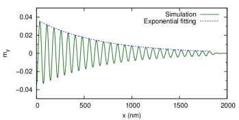
Figure 1: The spin wave amplitude decay along the rod, for a spin wave was excited locally by applying a microwave $\mathbf{H}=H_{0}\sin(2\pi ft)\mathbf{e}_{y}$ of frequency $f=30\,\mathrm{GHz}$ and amplitude $H_{0}=1000\,\mathrm{Oe}$ in the region $0\leq x\leq 2\,\mathrm{nm}$. The data were fitted using Eq. (23) with $\beta=0.02$ and $\alpha=0.01$.

Figure 1 illustrates the spin wave amplitude decay along the rod. The $y$ component of magnetization unit vector $m_{y}$ data for $30\leq x\leq 1800$ nm were fitted using (23) to extract the wave vector $k$ and the decay constant $\lambda$, and good agreement is observed due to the effective absence of spin wave reflection. We use data after having computed the time development of the magnetization for 4 ns to reach a steady state. The injected spin wave energy is absorbed efficiently enough within the right 200 nm of the rod due to the increased damping.

To analyze the simulation data, we exploit the uniform plane wave assumption with its exponential amplitude decay due to energy dissipation, i.e. magnetization with the form $e^{i(\mathrm{k}x-\omega t)}e^{-\lambda x}$, where $\lambda$ is the characteristic parameter of the spin wave damping. For a small amplitude spin wave propagation we have Seo et al. (2009)

$$\mathbf{m}=\mathbf{e}_{\mathrm{x}}+\mathbf{m}_{0}e^{i(kx-\omega t)}e^{-\lambda x}$$ (23)

where $|\mathbf{m}_{0}|\ll 1$, and the effective field of the long rod can be expressed as

$$\mathbf{H}_{\mathrm{eff}}=H_{s}m_{x}\mathbf{e}_{x}+D\nabla^{2}\mathbf{m},$$ (24)

where the ‘easy axis’ anisotropy field $H_{s}m_{x}\mathbf{e}_{x}$ originates from the demagnetizing field, and the constant $D$ measures the strength of the exchange field,

$$H_{s}=\frac{2K}{\mu_{0}M_{e}}=\frac{1}{2}M_{e},\qquad D=\frac{2A}{\mu_{0}M_{e}}.$$ (25)

To test the spin wave decay for this system, a sinusoidal field $\mathbf{H}=H_{0}\sin(2\pi ft)\mathbf{e}_{y}$ was applied to the rod in the region $0\leq x\leq 2\,\mathrm{nm}$ to generate spin waves.

Figure 2: The spin wave decay constant–wave vector product $\lambda k$ as a function of the frequency for different $\beta$ values. The slateblue line was drawn using Eq. (29) for the case $\beta=0.01$.

Figure 2 shows the product of spin wave decay constant $\lambda$ and wave vector $k$ as a function of the frequency. The dependence is linear for the $\beta=0$ case, which is agreement with the zero adiabatic spin torque case Seo et al. (2009). The addition of a nonzero $\beta$ term leads to a nonlinear relation, and the amplitude of the spin wave decay constant that is significantly larger than that given by the linear dependence. We also performed the simulation for $\chi>0$ case by using Eq. (5) which shows that $\beta$ term is the leading factor for this nonlinearity (the relative error is less than 1% for $\chi=1\times 10^{-3}$). To analyze the nonlinear dependence, we introduce the complex wave vector $\widetilde{k}$,

$$\widetilde{k}=k+\lambda i.$$ (26)

By linearizing Eq. (17) and setting the determinant of the matrix to zero we obtained (see Appendix B for details):

$$(\omega+\tilde{\omega}_{0}+i\tilde{\omega}_{1})(\omega-\tilde{\omega}_{0}+i\tilde{\omega}_{1})=0,$$ (27)

where $\tilde{\omega}_{0}=\gamma(H_{s}+D\tilde{k}^{2})$ and $\tilde{\omega}_{1}=\alpha\tilde{\omega}_{0}+\beta G\tilde{k}^{2}\tilde{\omega}_{0}$. The second term of the Eq. (27) is expected to be equal to zero, i.e., $\tilde{\omega}_{1}-i\omega+i\tilde{\omega}_{0}=0$. There are two scenarios to consider: First is the $\beta=0$ case, $k\lambda$ could be extracted by taking the imaginary part of $\tilde{k}^{2}$ at Eq. (26):

$$k\lambda=\frac{1}{2}\,\mathrm{Im}\left\{\tilde{k}^{2}\right\}=\frac{\alpha\omega}{2(1+\alpha^{2})\gamma D}.$$ (28)

The linear dependence of $k\lambda$ as a function of frequency matches the data plotted in Fig. 2. For the $\beta>0$ case, solving Eq. (27) yields in the linear with respect to the damping constants approximation,

$$k\lambda\approx\frac{\omega}{2\gamma D}(\alpha+\beta Gk^{2})$$ (29)

where the dispersion relation for the rod is $\omega=\gamma(H_{s}+Dk^{2})$. Eq. (29) shows there is an extra $k^{2}$ term associated with the exchange damping term besides the linear dependence between $k\lambda$ and $\omega$. The slateblue line in Fig. 2 is plotted using Eq. (29) with $\beta=0.01$ and $\alpha=0.01$, which shows a good approximation for the simulation data. Besides, this exchange damping could be important in determining the nonadiabatic spin torque. We could establish the value of $\beta$ using the existing experimental data, such as the transverse spin current data Nembach et al. (2013) gives $\beta\sim 0.1$ which hints the lifetime and propagation length of short-wavelength magnons could be much shorter than those given by the LLG equation Baryakhtar (2014).

IV Suppression of standing spin waves

In the presence of nonlocal damping, the high frequency standing spin waves in the thin films are suppressed Baryakhtar (2014). If the magnetization at the surfaces are pinned, the spin wave resonance can be excited by a uniform alternating magnetic field Kittel (1958). With given out-of-plane external field $H_{z}$ in the $z$-direction, the frequencies of the excited spin waves of the film are given by Stancil and Prabhakar (2009),

$$\omega_{n}=\omega_{0}+\omega_{M}\lambda_{\mathrm{ex}}^{2}\left(\frac{n\pi}{d}\right)^{2}$$ (30)

where $d$ is the film thickness, $\omega_{0}=\gamma(H_{z}-M_{e})$, $\omega_{M}=\gamma M_{e}$ and $\lambda_{\mathrm{ex}}=\sqrt{2A/(\mu_{0}M_{e}^{2})}$. The excited spin wave modes are labeled by the integer $n$, and the odd $n$ has a nonvanishing interaction with the given uniform alternating magnetic field Kittel (1958).

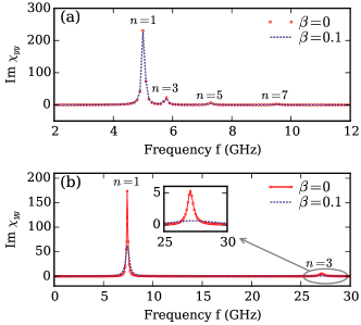
Figure 3: Imaginary parts of the dynamical susceptibility $\chi_{yy}$ of the film for (a) thickness $d=300$ nm, and (b) thickness $d=60$ nm.

To reduce the simulation time, we consider a system with cross-sectional area $4\times 4$ nm² in $xy$-plane and apply the two-dimensional periodic boundary conditions Wang et al. (2010) to the system. We use the Permalloy as the simulation material with external field $H_{z}=1\times 10^{6}$ A/m and the cell size is $4\times 4\times 2$ nm³. Instead of applying microwaves to the system, we calculate the magnetic absorption spectrum of the film by applying a sinc-function field pulse $h=h_{0}\mathrm{sinc}(\omega_{0}t)$ to the system Dvornik et al. (2013b). With the collected average magnetization data, the dynamic susceptibility $\chi$ is computed using Fourier transformation Liu et al. (2008). For example, the component $\chi_{yy}$ is computed using $m_{y}$ when the pulse is parallel to the $y$-axis.

Figure 3(a) shows the imaginary part of the dynamic susceptibility $\chi_{yy}$ for a film with $d=300$ nm. As we can see, the spin wave of modes $n=1,3,5,\dots$ are excited, and the influence of the “exchange damping” is small. However, the presence of the “exchange damping” suppresses the spin wave excitation ($n>1$ mode) significantly for the film with thickness $d=60$ nm, as shown in Fig. 3(b). The reason is because the damping of the standing spin waves is proportional to $k^{4}$ in the presence of exchange damping Baryakhtar (2014).

V Domain wall motion

We implemented Eq. (5) in a finite element based micromagnetic framework to study the effect of parallel relaxation process on domain wall motion. The simulated system for the domain wall motion is a one-dimensional (1D) mesh with length 20000 nm and discretization size $4\,\mathrm{nm}$, a head-to-head domain wall is initialized with its center near $x=500$ nm. In this section, the demagnetizing fields are simplified as $\mathbf{H}_{\mathrm{d}}=-N\mathbf{M}$ and the demagnetizing factors are chosen to be $N_{x}=0$, $N_{y}=0.2$ and $N_{z}=0.8$, respectively. The domain wall moves under the applied field for $50$ ns and the domain wall velocities at different external field strengths are computed. Figure 4 shows the simulation results of domain wall motion under external fields for different susceptibilities without consideration of exchange damping, i.e., $\beta=0$. For Nickel and Permalloy, the longitudinal susceptibility is around $10^{-4}$ at room temperature and increases with the temperature up until the Curie point Atxitia and Chubykalo-Fesenko (2011). We find that the longitudinal susceptibilities have no influence on the maximum velocity but change the Walker breakdown field $H_{w}$ significantly. The domain wall velocity in the limit $\chi\rightarrow 0$ is almost the same with the case of $\chi=10^{-4}$, which could be explained by the relation that the difference proportional to the ratio of $(\chi/\alpha)^{2}$ in Eq. (53).

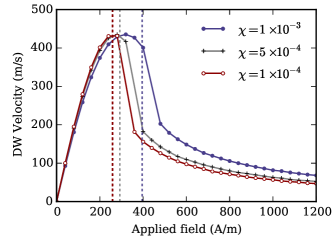
Figure 4: Simulations results of domain wall velocities for various susceptibilities. The parameters used are: $\alpha=0.001$, $\beta=0$, $N_{y}=0.2$ and $N_{z}=0.8$. The vertical dash lines are the breakdown fields computed using Eq. (53).

To investigate the effect of longitudinal magnetic susceptibility $\chi$ and exchange relaxation damping $\sigma$ on the domain wall motion, we use the remainder of this section for analytical studies. We start from the constant saturation magnetization of one-dimensional domain wall model, such as the 1D head-to-head wall Nakatani et al. (2005). The static 1D domain wall profile can be expressed as

$$m_{x}=-\tanh\left(\frac{x-q}{\Delta}\right),\quad m_{t}=\mathrm{sech}\left(\frac{x-q}{\Delta}\right)$$ (31)

where $m_{t}$ is the perpendicular component of the unit magnetization vector, $\Delta$ is the wall width parameter and $q$ is the position of the domain wall center.

We consider the case that the system is characterized by two anisotropies, easy uniaxial anisotropy $K$ and hard plane anisotropy $K_{\perp}$, which originate from demagnetization. The aim is to analyze the impact of the longitudinal magnetic susceptibility under the 1D domain wall model, the demagnetization energy density could be written as

$$E_{\mathrm{an}}=-\frac{K}{M_{e}^{2}}M_{x}^{2}+\frac{K_{\perp}}{M_{e}^{2}}M_{z}^{2}$$ (32)

where $K=(1/2)(N_{y}-N_{x})\mu_{0}M_{e}^{2}$ and $K_{\perp}=(1/2)(N_{z}-N_{y})\mu_{0}M_{e}^{2}$. In the limit case $\chi\rightarrow 0$ case, the effective anisotropy energy density $E_{\mathrm{an}}$ can be rewritten as

$$E^{\prime}_{\mathrm{an}}=K\sin^{2}\theta(1+\kappa\sin^{2}\varphi),$$ (33)

where $\mathbf{m}=(\cos\theta,\sin\theta\cos\varphi,\sin\theta\sin\varphi)$ is used and $\kappa=K_{\perp}/K$ is the ratio between hard plane anisotropy strength and easy uniaxial anisotropy strength.

The dynamics of the domain wall with 1D profile can be described using 3 parameters O’Brien et al. (2012): the domain width $\Delta$, the domain wall position $q$ and the domain wall tilt angle $\phi$. In this domain wall model, one can assume that $\varphi(x,t)=\phi(t)$ is only a function of time. Thus, the magnetization profile for the head-to-head domain wall is given by

$$\theta(x,t)=2\tan^{-1}\exp\left(\frac{x-q(t)}{\Delta(t)}\right),\quad\varphi(x,t)=\phi(t).$$ (34)

Using the magnetization unit vector to calculate the exchange energy is a good approximation for the case $\chi\ll 1$, thus, the total energy density can be rewritten as

$$E_{\mathrm{tot}}=\frac{\mu_{0}}{8\chi}\frac{(M^{2}-M_{e}^{2})^{2}}{M_{e}^{2}}+M^{2}w_{\mu}(\mathbf{m}),$$ (35)

where

$$w_{\mu}(\mathbf{m})=\frac{A}{M_{e}^{2}}(\nabla\mathbf{m})^{2}-\frac{K}{M_{e}^{2}}m_{x}^{2}+\frac{K_{\perp}}{M_{e}^{2}}m_{z}^{2}.$$ (36)

Within the 1D domain wall profile, $H_{\mathrm{m}}$, the longitudinal component of the effective field is obtained:

$$H_{\mathrm{m}}=\mathbf{m}\cdot\mathbf{H}_{\mathrm{eff}}=\frac{M}{2\chi M_{e}^{2}}(M_{e}^{2}-M^{2})-2MP\sin^{2}\theta$$ (37)

where $P$ is defined as

$$P=\frac{1}{\mu_{0}M_{e}^{2}}\left[\frac{A}{\Delta^{2}}+K(1+\kappa\sin^{2}\phi)\right].$$ (38)

As we can see, $P$ is a function of the tilt angle $\phi$ and the domain wall width $\Delta$. At the static state, $H_{m}$ should equal zero, i.e., ${dM}/{dt}=0$, which gives

$$M^{2}=(1-4\chi P\sin^{2}\theta)M_{e}^{2}.$$ (39)

Eq. (39) shows that the difference between magnetization length $M$ and $M_{e}$ reaches its maximum at the center of the domain wall due to the effect of the exchange field, which also peaks in the centre of the domain wall. According to Eq. (39), we can estimate that the magnetization length difference is $\delta M\approx-2\chi P\sin^{2}\theta$ for $\chi\ll 1$ case. Figure 5 shows the magnetization length differences of a 1D domain wall for various $\chi$, it can be seen that this approximation for $\delta M$ agrees very well with the simulation results.

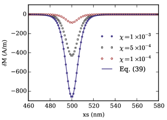
Figure 5: Simulation results of the magnetization length difference $\delta M$ for a 1D domain wall located at $x=500$ nm with $M_{e}=8.6\times 10^{5}\,\mathrm{A/m}$ and $A=1.3\times 10^{-11}$ J/m. The demagnetizing factors are selected to be $N_{x}=0$ and $N_{y}=N_{z}=0.5$.

In the dynamic case, $H_{m}$ is not equal to zero. If we wrote Eq. (37) as $H_{\mathrm{m}}=FM$, we can find that the nontrivial term that contributes to $H_{m}$ is

$$F=\frac{1}{2\chi}(1-M^{2}/M_{e}^{2})-2P\sin^{2}\theta.$$ (40)

As an approximation for $H_{\mathrm{m}}$, we expect $dF/dt=0$ Sobolev et al. (1997), which gives

$$H_{\mathrm{m}}=\frac{4P}{\Delta}\frac{\chi}{\alpha}\frac{\dot{q}}{\gamma}m_{t}^{2}m_{x}.$$ (41)

In this approximation, we have ignored the terms containing $dP/dt$ and thus the amplitude of $H_{\mathrm{m}}$ is influenced by the domain wall velocity $\dot{q}$ only. We employ the Lagrangian equation combined with dissipation function $\mathcal{F}$ to compute the domain wall dynamics Hillebrands and Thiaville (2006). The Lagrange equations are

$$\frac{\partial\mathcal{L}}{\partial X}-\frac{d}{dt}\left(\frac{\partial\mathcal{L}}{\partial\dot{X}}\right)+\frac{\partial\mathcal{F}}{\partial\dot{X}}=0,$$ (42)

where $X$ refers to $q$, $\phi$ and $\Delta$. The dissipation function is defined by $\mathcal{F}=\int\!F\,dx$ where

$$F=\frac{1}{2}\mu_{0}M_{e}\gamma[\alpha\mathbf{H}_{\mathrm{eff}}^{2}+\sigma(\nabla\mathbf{H}_{\mathrm{eff}})^{2}]$$ (43)

is the dissipation density function.

V.1 Parallel relaxation

We neglect the exchange damping term with assumption that $\sigma\ll\alpha\Delta^{2}$ and arrive at

$$F=\frac{1}{2}\alpha\mu_{0}M_{e}\gamma\mathbf{H}_{\mathrm{eff}}^{2}=\frac{1}{2}\alpha\mu_{0}M_{e}\gamma(\mathbf{H}_{\perp}^{2}+\mathbf{H}_{m}^{2}).$$ (44)

where $\mathbf{H}_{\perp}$ and $\mathbf{H}_{m}$ are the perpendicular and parallel components of the effective field. If we also assume that $\alpha\sim\chi\ll 1$, $\mathbf{H}_{\perp}^{2}$ can be approximated by Eq. (11),

$$\mathbf{H}_{\perp}^{2}=\frac{1}{\gamma^{2}}\dot{\mathbf{m}}^{2}=\frac{1}{\gamma^{2}}(\dot{\theta}^{2}+\sin^{2}\theta\dot{\phi}^{2}).$$ (45)

Substituting Eq. (41) and Eq. (45) into Eq. (44) and integrating over space, we obtain

$$\mathcal{F}=\frac{\alpha\mu_{0}M_{e}}{\gamma}\left[\dot{\phi}^{2}\Delta+\frac{\dot{q}^{2}}{\Delta}(1+Q)\right],$$ (46)

where we have ignored the $\dot{\Delta}$ term. This term leads to the optimal domain wall width Hillebrands and Thiaville (2006):

$$\Delta=\sqrt{A/(K+K_{\perp}\sin^{2}\phi)}$$ (47)

and for $\kappa=0$ the optimal domain wall width reduces to $\Delta_{0}=\sqrt{A/K}$. In what follows, the domain wall width parameter $\Delta(t)$ is approximated by the optimal wall width. The parameter $P$ is then given by

$$P=\frac{2K(1+\kappa\sin^{2}\phi)}{\mu_{0}M_{e}^{2}}=\frac{2}{\mu_{0}M_{e}^{2}}\frac{A}{\Delta^{2}},$$ (48)

and it is straightforward to find its minimum $P_{0}=2K/(\mu_{0}M_{e}^{2})$, which corresponds to $\Delta=\Delta_{0}$.

The introduced paramter $Q$ in Eq. (46) is given by $Q=(32/15)P^{2}(\chi/\alpha)^{2}$ and its value is determined by the ratio of $\chi$ and $\alpha$, which could be $\sim 1$ although we assume $\chi\sim\alpha\ll 1$. Following the treatment of Ref. [27], the integrated Lagrangian action $\mathcal{L}$ is given by

$$\begin{split}\mathcal{L}&=\int\!(E_{\mathrm{tot}}+\frac{\mu_{0}M_{e}}{\gamma}\dot{\phi}\cos\theta)\,dx\\ &=\frac{2A}{\Delta}+2\Delta K(1+\kappa\sin^{2}\phi)(1-V)\\ &\qquad-2\mu_{0}M_{e}H_{a}q+\frac{2\mu_{0}M_{e}}{\gamma}\dot{\phi}q,\end{split}$$ (49)

where $\mu_{0}M_{e}\dot{\phi}\cos\theta/\gamma$ is the Berry phase term Shibata et al. (2011), $V=8\chi P/3$ is a result of the varying magnetization that introduced a pinning potential. However, the potential is fairly small and therefore is negligible since $V\ll Q$. By substituting Eq. (49) and Eq. (44) into Eq. (42),

$$\begin{split}&\dot{\phi}+\alpha\frac{\dot{q}}{\Delta}\left(1+Q\right)=\gamma H_{a},\\ &\frac{\dot{q}}{\Delta}-\alpha\dot{\phi}=\gamma\frac{H_{k}}{2}\sin 2\phi.\end{split}$$ (50)

where $H_{k}=2K_{\perp}/(\mu_{0}M_{e})$. The domain wall dynamics is governed by Eq. (50), by eliminating $\dot{q}$ we obtain an equation about $\phi$,

$$\dot{\phi}=\frac{\gamma}{1+\alpha^{2}(1+Q)}\left[H_{a}-H_{w}(1+Q)\sin 2\phi\right]$$ (51)

where $H_{w}=\alpha H_{k}/2$ is the Walker breakdown field. From Eq. (51) we can find that the critical value of $\phi$ is approximately equal to $\pi/4$ if $Q\ll 1$, which leads to the maximum value of $P$ to be $P_{1}=2K(1+\kappa/2)/(\mu_{0}M_{e}^{2})$. There exists an equilibrium state $\phi^{*}$ such that $\dot{\phi}=0$ if $H_{a}<H_{w}(1+Q)$,

$$\sin(2\phi^{*})=h\equiv\frac{H_{a}}{H_{w}(1+Q)},$$ (52)

which means the Walker breakdown field $H^{\prime}_{w}$ for $\chi>0$ case is increased to $H_{w}(1+\max\{Q\})$, i.e.,

$$H^{\prime}_{w}=H_{w}\left[1+\frac{32}{15}P_{1}^{2}\left(\frac{\chi}{\alpha}\right)^{2}\right],$$ (53)

where $P_{1}$ is the maximum vlaue of $P$. For this steady-state wall motion, the domain wall velocity is

$$\dot{q}=\frac{\gamma H_{a}}{\alpha}\frac{\Delta^{*}}{1+Q(\Delta^{*})},$$ (54)

where

$$\Delta^{*}=\Delta_{0}/\sqrt{1+\frac{\kappa}{2}(1-\sqrt{1-h^{2}})}.$$ (55)

Therefore, $\Delta^{*}\rightarrow\Delta_{0}$ in the limit case $H_{a}\rightarrow 0$, and the domain wall mobility $\mu$ is given by

$$\mu=\frac{\gamma\Delta}{\alpha}\left[1+\frac{32}{15}P_{0}^{2}(\frac{\chi}{\alpha})^{2}\right]^{-1}$$ (56)

where $P_{0}$ is the minimum value of $P$. In Fig. 4 the corresponding Walker breakdown fields are plotted in vertical dash lines, which gives a good approximation for $\chi=5\times 10^{-4}$ and $\chi=1\times 10^{-4}$ cases. The simulation results show that the Walker breakdown field $H_{w}$ could be changed significantly if the longitudinal susceptibility is comparable to the damping constant.

V.2 Nonlocal damping

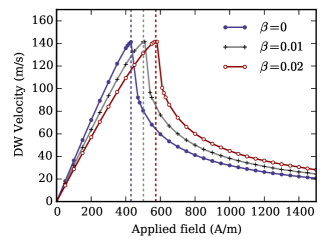
Figure 6: Simulations results of domain wall velocities for the limit case that $\chi\rightarrow 0$ with various exchange dampings. The parameters used are: $\alpha=0.005$, $N_{y}=0.4$ and $N_{z}=0.6$. The vertical dash lines are the breakdown fields computed with Eq. (60).

In this part we consider the domain wall motion influenced by exchange damping for the case that $\chi\rightarrow 0$. The dissipation density function (43) thus becomes

$$F=\frac{1}{2}\mu_{0}M_{e}\gamma\left[\alpha\mathbf{H}_{\perp}^{2}+\sigma(\nabla H_{\theta})^{2}+\sigma(\nabla H_{\phi})^{2}\right]$$ (57)

where $H_{\theta}$ and $H_{\phi}$ are the two components of the effective field, and $\mathbf{H}_{\perp}$ is computed using Eq. (45). After calculation we obtain

$$\mathcal{F}=\frac{\mu_{0}M_{e}}{\gamma}\left[\dot{\phi}^{2}(\alpha\Delta+\frac{1}{3}\frac{\sigma}{\Delta})+\frac{\dot{q}^{2}}{\Delta}(\alpha+\frac{1}{3}\frac{\sigma}{\Delta^{2}})\right].$$ (58)

We take the same Lagrangian action (49) for $\chi=0$ and arrive at

$$\begin{split}&\dot{\phi}+(\alpha+\frac{\sigma}{3\Delta^{2}})\frac{\dot{q}}{\Delta}=\gamma H_{a},\\ \frac{\dot{q}}{\Delta}&-(\alpha+\frac{\sigma}{3\Delta^{2}})\dot{\phi}=\gamma\frac{H_{k}}{2}\sin 2\phi.\end{split}$$ (59)

Similarly, the corresponding Walker breakdown field changes to

$$H^{\prime}_{w}=\frac{1}{2}H_{k}\left(\alpha+\frac{1}{3}\frac{\sigma}{\Delta^{2}_{1}}\right),$$ (60)

where $\Delta_{1}=\Delta_{0}\sqrt{1/(1+\kappa/2)}$. The domain wall mobility is given by

$$\frac{1}{\mu}=\frac{1}{\gamma\Delta_{0}}\left(\alpha+\frac{1}{3}\frac{\sigma}{\Delta^{2}_{0}}\right).$$ (61)

As we can see, the nonlocal damping term $\sigma$ influences the domain wall motion as well, and we can establish that $\sigma/\Delta^{2}=\beta(1+\kappa/2)K/(\mu_{0}M_{e}^{2})\propto\beta$. Therefore, for the scenarios that $K\sim\mu_{0}M_{e}^{2}$, the contributions from the Gilbert and nonlocal damping are of the order of magnitude for both the domain wall mobility and Walker breakdown field.

Figure 6 shows the domain wall velocities for domain wall motion driven by external fields in the limiting case of $\chi\rightarrow 0$. The simulation results are based on a one-dimensional mesh with length $10000$ nm with cell size of $2$ nm. The damping $\alpha$ is set to $0.005$ and the demagnetizing factors are chosen to be $N_{x}=0$, $N_{y}=0.4$ and $N_{z}=0.6$. As predicted by Eq. (60), the nonlocal damping $\beta$ leads to an increment of the Walker breakdown field, and Eq. (60) fits the simulation results very well.

VI Summary

We explain the “exchange damping” in the Landau-Lifshitz-Baryakhtar (LLBar) equation as nonlocal damping by linking it to the spin current pumping, and therefore the LLBar (17) can be considered as a phenomenological equation to describe the nonlocal damping. In the presence of nonlocal damping, the lifetime and propagation length of short-wavelength magnons could be much shorter than those given by the LLG equation. Our simulation results show that the spin wave amplitude decays much faster in the presence of nonlocal damping when spin waves propagate along a single rod. The analytical result shows that there is extra nonlinear dependence scaling with $k^{2}$ between $\lambda k$ (the product of spin wave decay constant $\lambda$ and wave vector $k$) and frequency $\omega$ due to the nonlocal damping. Using the micromagnetic simulation based on the LLBar equation, we show that the difference between magnetization length $M$ and $M_{e}$ reaches its maximum at the center of the domain wall. For the cases that $\chi\sim\alpha$ where $\chi$ is the longitudinal magnetic susceptibility and $\alpha$ is the Gilbert damping, the Walker breakdown field will increase significantly. By using a 1D domain wall model, we also show that both the domain wall mobility and the Walker breakdown field are strongly influenced by the nonlocal damping as well.

Appendix A Derivation of equation (II)

We split the perpendicular spin current $\mathbf{j}_{\perp,i}$ into two components,

$$\mathbf{j}_{\perp,i}=\mathbf{j}_{i}^{a}+\mathbf{j}_{i}^{b},$$ (62)

where we write $\lambda_{e}/\gamma$ as $\tilde{\sigma}$,

$$\mathbf{j}_{i}^{a}=-\tilde{\sigma}(\partial_{i}\mathbf{m}\times\partial_{t}\mathbf{m})$$ (63)

$$\mathbf{j}_{i}^{b}=-\tilde{\sigma}(\mathbf{m}\times\partial_{i}\partial_{t}\mathbf{m})$$ (64)

The torque $\bm{\tau}_{a}$ generated by spin current $\mathbf{j}_{i}^{a}$ is given by $\bm{\tau}_{a}=(\partial_{i}\mathbf{j}_{i}^{a})_{\perp}$, i.e.,

$$\bm{\tau}_{a}=\tilde{\sigma}\mathbf{m}\times[\partial_{i}\mathbf{m}\times(\partial_{t}\mathbf{m}\times\partial_{i}\mathbf{m})]$$ (65)

where we have used the identities $\mathbf{m}\cdot\partial_{i}\partial_{t}\mathbf{m}=-\partial_{i}\mathbf{m}\cdot\partial_{t}\mathbf{m}$ and $\mathbf{m}\cdot\partial_{i}\partial_{i}\mathbf{m}=-\partial_{i}\mathbf{m}\cdot\partial_{i}\mathbf{m}$. Meanwhile, the corresponding torque $\bm{\tau}_{b}$ can be computed by $\bm{\tau}_{b}=(\partial_{i}\mathbf{j}_{i}^{b})_{\perp}$, which gives

$$\bm{\tau}_{b}=\bm{\tau}_{a}-\tilde{\sigma}(\partial_{i}\mathbf{m}\cdot\partial_{i}\mathbf{m})\mathbf{m}\times\partial_{t}\mathbf{m}-\tilde{\sigma}\mathbf{m}\times\nabla^{2}\partial_{t}\mathbf{m}$$ (66)

Note that $\bm{\tau}_{a}=\tilde{\sigma}\partial_{i}\mathbf{m}[(\partial_{t}\mathbf{m}\times\partial_{i}\mathbf{m})\cdot\mathbf{m}]$ can be changed into the tensor form,

$$\bm{\tau}_{a}=\mathbf{m}\times(\mathcal{D}^{0}\cdot\partial_{t}\mathbf{m}),$$ (67)

where

$$\mathcal{D}^{0}_{\alpha\beta}=\tilde{\sigma}(\mathbf{m}\times\partial_{i}\mathbf{m})_{\alpha}(\mathbf{m}\times\partial_{i}\mathbf{m})_{\beta}.$$ (68)

Therefore, we obtain for $\bm{\tau}_{a}+\bm{\tau}_{b}$,

$$\bm{\tau}_{a}+\bm{\tau}_{b}=\mathbf{m}\times(\mathcal{D}\cdot\partial_{t}\mathbf{m})-\tilde{\sigma}\mathbf{m}\times\nabla^{2}\partial_{t}\mathbf{m}$$ (69)

where $\mathcal{D}$ is a $3\times 3$ tensor,

$$\mathcal{D}_{\alpha\beta}=2\tilde{\sigma}(\mathbf{m}\times\partial_{i}\mathbf{m})_{\alpha}(\mathbf{m}\times\partial_{i}\mathbf{m})_{\beta}-\tilde{\sigma}(\partial_{i}\mathbf{m}\cdot\partial_{i}\mathbf{m})\delta_{\alpha\beta}.$$ (70)

Appendix B Derivation of equation (27)

We introduce a new variable $\mathbf{s}$ to represent the second term in the (23), i.e., $\mathbf{s}=\mathbf{m}_{0}e^{i(\tilde{k}x-\omega t)}$, so we have

$$\mathbf{m}=\mathbf{e}_{\mathrm{x}}+\mathbf{s},$$ (71)

$$\frac{d\mathbf{m}}{dt}=-i\,\omega\,\mathbf{s},$$ (72)

$$\mathbf{H}_{\mathrm{eff}}=H_{s}(1+s^{\prime}_{x})\mathbf{e}_{\mathrm{x}}-D\tilde{k}^{2}\mathbf{s}$$ (73)

where $s^{\prime}_{x}\approx(1/2)(s_{x}^{2}-s^{2})$. Considering the fact $|\mathbf{s}|\ll 1$ and neglect the high order term $s^{2}$, one obtains $\mathbf{H}_{\mathrm{eff}}^{\perp}=-(H_{s}+D\tilde{k}^{2})\mathbf{s}$ and thus

$$\mathbf{H}_{\mathrm{eff}}^{b}=c\,\mathbf{e}_{\mathrm{x}}+d\,\mathbf{s}$$ (74)

where

$$c=\alpha H_{s}(1+s^{\prime}_{x}),$$ (75)

$$d=-\beta G\tilde{k}^{2}(D\tilde{k}^{2}+H_{s})-\alpha D\tilde{k}^{2}$$ (76)

Substituting the above equations into (17), we have

$$\frac{i\omega}{\gamma}\left[\begin{array}[]{c}s_{x}\\ s_{y}\\ s_{z}\end{array}\right]=f\left[\begin{array}[]{c}0\\ s_{z}\\ -s_{y}\end{array}\right]+(c-d)\left[\begin{array}[]{c}-(s_{y}^{2}+s_{z}^{2})\\ (1+s_{x})s_{y}\\ (1+s_{x})s_{z}\end{array}\right],$$ (77)

where $f=H_{s}(1+s^{\prime}_{x})+D\tilde{k}^{2}$. Neglecting high order terms such as $s_{x}^{2}$ and $s_{x}s_{y}$ we obtained,

$$\begin{bmatrix}\gamma(\alpha H_{s}-d)-i\omega&\tilde{w}_{0}\\ -\tilde{w}_{0}&\gamma(\alpha H_{s}-d)-i\omega\end{bmatrix}\begin{bmatrix}s_{y}\\ s_{z}\end{bmatrix}=\begin{bmatrix}0\\ 0\end{bmatrix}.$$ (78)

Therefore, Eq. (27) can be obtained by setting the determinant of the matrix in (78) to zero.

References

- Landau and Lifshitz (1935) L. Landau and E. Lifshitz, Phys. Z. Sowjetunion 169, 14 (1935).
- Akhiezer et al. (1968) A. I. Akhiezer, V. G. Bar’yakhtar, and S. V. Peletminskii, Spin waves (North-Holland, Amsterdam, 1968).
- Donahue and Porter (1999) M. Donahue and D. Porter, “OOMMF User’s Guide, Version 1.0,” (1999), http://math.nist.gov/oommf/.
- Scholz et al. (2003) W. Scholz, J. Fidler, T. Schrefl, D. Suess, R. Dittrich, H. Forster, and V. Tsiantos, Comput. Mater. Sci. 28, 366 (2003).
- Fischbacher et al. (2007) T. Fischbacher, M. Franchin, G. Bordignon, and H. Fangohr, IEEE Trans. Magn. 43, 2896 (2007).
- Berkov and Gorn (2008) D. V. Berkov and N. L. Gorn, J. Phys. D. Appl. Phys. 41, 164013 (2008).
- Vansteenkiste et al. (2014) A. Vansteenkiste, J. Leliaert, M. Dvornik, M. Helsen, F. Garcia-Sanchez, and B. Van Waeyenberge, AIP Advances 4, 107133 (2014).
- Gilbert (2004) T. Gilbert, IEEE Trans. Magn. 40, 3443 (2004).
- García-Palacios and Lázaro (1998) J. L. García-Palacios and F. J. Lázaro, Phys. Rev. B 58, 14937 (1998).
- Shu et al. (2004) Y. Shu, M. Lin, and K. Wu, Mech. Mater. 36, 975 (2004).
- Zhang and Li (2004) S. Zhang and Z. Li, Phys. Rev. Lett. 93, 127204 (2004).
- Thiaville et al. (2005) A. Thiaville, Y. Nakatani, J. Miltat, and Y. Suzuki, Europhys. Lett. 69, 990 (2005).
- Lebecki et al. (2008) K. M. Lebecki, M. J. Donahue, and M. W. Gutowski, J. Phys. D. Appl. Phys. 41, 175005 (2008).
- Wang et al. (2010) W. Wang, C. Mu, B. Zhang, Q. Liu, J. Wang, and D. Xue, Comput. Mater. Sci. 49, 84 (2010).
- Krueger and Selke (2013) B. Krueger and G. Selke, IEEE Trans. Magn. 49, 4749 (2013).
- Kirilyuk et al. (2010) A. Kirilyuk, A. V. Kimel, and T. Rasing, Rev. Mod. Phys. 82, 2731 (2010).
- Au et al. (2013) Y. Au, M. Dvornik, T. Davison, E. Ahmad, P. Keatley, A. Vansteenkiste, B. Van Waeyenberge, and V. Kruglyak, Phys. Rev. Lett. 110, 097201 (2013).
- Terris and Thomson (2005) B. D. Terris and T. Thomson, J. Phys. D. Appl. Phys. 38, R199 (2005).
- Kruglyak et al. (2010) V. V. Kruglyak, S. O. Demokritov, and D. Grundler, J. Phys. D. Appl. Phys. 43, 264001 (2010).
- Baryakhtar (1998) V. Baryakhtar, in Front. Magn. Reduc. Dimens. Syst. (1998) pp. 63–94.
- Bar’yakhtar et al. (1986) V. G. Bar’yakhtar, B. A. Ivanov, T. K. Soboleva, and A. L. Sukstanskii, Zh. Éksp. Teor. Fiz 64, 857 (1986).
- Baryakhtar and Danilevich (2013) V. G. Baryakhtar and A. G. Danilevich, Low Temp. Phys. 39, 993 (2013).
- Zhang and Zhang (2009) S. Zhang and S. S.-L. Zhang, Phys. Rev. Lett. 102, 086601 (2009).
- De Angeli et al. (2009) L. De Angeli, D. Steiauf, R. Singer, I. Köberle, F. Dietermann, and M. Fähnle, Phys. Rev. B 79, 052406 (2009).
- Dvornik et al. (2013a) M. Dvornik, A. Vansteenkiste, and B. Van Waeyenberge, Phys. Rev. B 88, 054427 (2013a).
- Yastremsky et al. (2014) I. A. Yastremsky, P. M. Oppeneer, and B. A. Ivanov, Phys. Rev. B 105, 024409 (2014).
- Hillebrands and Thiaville (2006) B. Hillebrands and A. Thiaville, Spin Dynamics in Confined Magnetic Structures III (Springer, New York, 2006).
- Weindler et al. (2014) T. Weindler, H. G. Bauer, R. Islinger, B. Boehm, J.-Y. Chauleau, and C. H. Back, Phys. Rev. Lett. 113, 237204 (2014).
- Atxitia and Chubykalo-Fesenko (2011) U. Atxitia and O. Chubykalo-Fesenko, Phys. Rev. B 84, 144414 (2011).
- Tserkovnyak et al. (2009) Y. Tserkovnyak, E. Hankiewicz, and G. Vignale, Phys. Rev. B 79, 094415 (2009).
- Fähnle and Zhang (2013) M. Fähnle and S. Zhang, J. Magn. Magn. Mater. 326, 232 (2013).
- Hankiewicz et al. (2008) E. Hankiewicz, G. Vignale, and Y. Tserkovnyak, Phys. Rev. B 78, 020404 (2008).
- Hickey and Moodera (2009) M. Hickey and J. Moodera, Phys. Rev. Lett. 102, 137601 (2009).
- Nembach et al. (2013) H. T. Nembach, J. M. Shaw, C. T. Boone, and T. J. Silva, Phys. Rev. Lett. 110, 117201 (2013).
- Han et al. (2009) D.-S. Han, S.-K. Kim, J.-Y. Lee, S. J. Hermsdoerfer, H. Schultheiss, B. Leven, and B. Hillebrands, Appl. Phys. Lett. 94, 112502 (2009).
- Seo et al. (2009) S.-M. Seo, K.-J. Lee, H. Yang, and T. Ono, Phys. Rev. Lett. 102, 147202 (2009).
- Baryakhtar (2014) V. G. Baryakhtar, Low Temp. Phys. 40, 626 (2014).
- Kittel (1958) C. Kittel, Phys. Rev. 110, 1295 (1958).
- Stancil and Prabhakar (2009) D. Stancil and A. Prabhakar, Spin Waves: Theory and Applications (Springer, 2009).
- Dvornik et al. (2013b) M. Dvornik, Y. Au, and V. V. Kruglyak, Top. Appl. Phys., 125, 101 (2013b).
- Liu et al. (2008) R. Liu, J. Wang, Q. Liu, H. Wang, and C. Jiang, J. Appl. Phys. 103, 013910 (2008).
- Nakatani et al. (2005) Y. Nakatani, A. Thiaville, and J. Miltat, J. Magn. Magn. Mater. 290, 750 (2005).
- O’Brien et al. (2012) L. O’Brien, E. Lewis, A. Fernández-Pacheco, D. Petit, R. Cowburn, J. Sampaio, and D. Read, Phys. Rev. Lett. 108, 187202 (2012).
- Sobolev et al. (1997) V. L. Sobolev, S. C. Chen, and H. L. Huang, J. Magn. Magn. Mater. 72, 83 (1997).
- Shibata et al. (2011) J. Shibata, G. Tatara, and H. Kohno, J. Phys. D. Appl. Phys. 44, 384004 (2011).