Distributed Resource Allocation for Relay-Aided Device-to-Device Communication Under Channel Uncertainties: A Stable Matching Approach

Abstract

Wireless device-to-device (D2D) communication underlaying cellular network is a promising concept to improve user experience and resource utilization. Unlike traditional D2D communication where two mobile devices in the proximity establish a direct local link bypassing the base station, in this work we focus on relay-aided D2D communication. Relay-aided transmission could enhance the performance of D2D communication when D2D user equipments (UEs) are far apart from each other and/or the quality of D2D link is not good enough for direct communication. Considering the uncertainties in wireless links, we model and analyze the performance of a relay-aided D2D communication network, where the relay nodes serve both the cellular and D2D users. In particular, we formulate the radio resource allocation problem in a two-hop network to guarantee the data rate of the UEs while protecting other receiving nodes from interference. Utilizing time sharing strategy, we provide a centralized solution under bounded channel uncertainty. With a view to reducing the computational burden at relay nodes, we propose a distributed solution approach using stable matching to allocate radio resources in an efficient and computationally inexpensive way. Numerical results show that the performance of the proposed method is close to the centralized optimal solution and there is a distance margin beyond which relaying of D2D traffic improves network performance.

I Introduction

We consider relay-assisted device-to-device (D2D) communication underlaying LTE-A cellular networks where D2D user equipments (UEs) are served by the relay nodes [1, 2]. When the link condition between two D2D UEs is too poor for direct communication, the D2D traffic can be transmitted via a relay node, which performs scheduling and resource allocation for the D2D UEs. We refer to this as relay-aided D2D communication which can be an efficient approach to provide better quality of service (QoS) for communication between distant D2D UEs. For this, we utilize the LTE-A Layer-3 (L3) relay  [3]. We consider scenarios in which the potential D2D UEs are located in the same macrocell; however, the proximity and link condition may not be favorable for direct communication. Therefore, they communicate via relays. The radio resources (e.g., resource blocks [RBs] and transmission power) at the relays are shared among the D2D communication links and the two-hop cellular links.

We formulate an optimization problem to allocate radio resources at a relay node in a muti-relay multi-user orthogonal frequency-division multiple access (OFDMA) cellular network (e.g., LTE-A network). Due to the NP-hardness of the resource allocation problem, we utilize time sharing strategy and provide an asymptotically optimal centralized solution. Considering the random nature of wireless channels, we reformulate the resource allocation problem using the worst-case robust optimization theory. The uncertainties in link gains are modeled using ellipsoidal uncertainty sets. Each relay node can centrally solve the problem taking channel uncertainty into consideration. However, considering the high (e.g., cubic to the number of UEs and RBs) computational overhead at the relay nodes, we provide a distributed solution based on stable matching theory which is computationally inexpensive (e.g., linear with the number of UEs and RBs). We also analyze the stability, uniqueness, and optimality of the proposed solution.

Considering the computational and signalling overheads and lack of scalability of the centralized solutions, game theoretical models have been widely used for wireless resource allocation problems. However, the analytical tractability of equilibrium in such game-theoretical models requires special properties for the objective functions, such as convexity, which may not be satisfied for many practical cases [4]. In this context, resource allocation using matching theory has several beneficial properties [5, 4]. For example, the stable matching algorithm terminates for every given preference profile. The outcome of matching provides suitable solutions in terms of stability and optimality, which can accurately reflect different system objectives. Besides, with suitable data structures, a Pareto optimal stable matching (e.g., allocation of resources to the UEs) can be obtained quickly for online implementation.

The goal of this work is to design a practical radio resource scheme for relay-aided D2D communication in a multi-user multi-relay OFDMA network. As opposed to most of the work in the literature where channel gain information is assumed to be perfect, we capture the dynamics of random and time-varying nature of wireless channels. To this end, we develop a low-complexity distributed solution based on the theory of stable matching and demonstrate how this scheme can be implemented in a practical LTE-A system. The major contributions of this work can be summarized as follows:

• We model and analyze the radio resource allocation problem for relay-aided D2D communication underlaying an OFDMA cellular network considering uncertainties in channel gains. We formulate an optimization problem to maximize system capacity in a two-hop network while satisfying the minimum data rate requirement for each UE and limiting the interference to other receiving nodes. We show that the convexity of the optimization problem is conserved under bounded channel uncertainty in both the useful and interference links.

• Using the theory of stable matching, we develop a distributed iterative solution, which considers bounded channel uncertainty. The stability, uniqueness, optimality, and complexity of the proposed solution are analyzed. We also present a possible implementation approach of our proposed scheme in an LTE-A system.

• Numerical results show that the proposed distributed solution performs close to the upper bound of the optimal solution obtained in a centralized manner; however, it incurs a lower (e.g., linear compared to cubic) computational complexity. Through simulations, we also compare the performance of the proposed approach with a traditional underlay D2D communication scheme and observe that after a distant margin, relaying of D2D traffic improves network performance.

We organize the rest of the paper as follows. We briefly review the related work in Section II. Section III presents the system model and related assumptions. Followed by the formulation of the nominal resource allocation problem in Section IV, we reformulate the resource allocation problem considering wireless channel gain uncertainties in Section V. We develop the stable matching-based distributed resource allocation algorithm in Section VI. Theoretical analysis of the proposed solution is presented in Section VII. In Section VIII, we present the performance evaluation results before we conclude the paper in Section IX.

II Related Work

TABLE I: Summary of Related Work and Comparison with Proposed Scheme

Reference	Problem focus	Relay-aided	Channel information	Solution approach	Solution type	Optimality
Work on D2D communication [6]	Resource allocation	No	Perfect	Proposed greedy heuristic	Centralized	Suboptimal
[7]	Resource allocation	No	Perfect	Column generation based greedy heuristic	Centralized	Suboptimal
[8]	Resource allocation	No*	Perfect	Numerical optimization	Semi-distributed	Pareto optimal
[9]	Resource allocation	No	Perfect	Interference graph coloring	Centralized	Suboptimal
[10]	Resource allocation	No	Perfect	Two-phase heuristic	Centralized	Suboptimal
[11]	Resource allocation, mode selection	No	Perfect	Particle swarm optimization	Centralized	Suboptimal
[12]	Resource allocation, mode selection	Yes	Perfect	Proposed heuristic	Distributed	Suboptimal
[13]	Theoretical analysis, performance evaluation	Yes	Perfect	Statistical analysis	Centralized	Optimal
[14]	Performance evaluation	Yes	Perfect	Heuristic, simulation	Centralized	N/A$\ddagger$
[1]	Resource allocation	Yes	Perfect	Numerical optimization	Centralized	Asymptotically optimal
[2]	Resource allocation	Yes	Uncertain#	Gradient-based iterative update	Distributed	Suboptimal
Work utilizes matching theory [15]	Resource allocation	N/A†	Perfect	One-to-one matching	Centralized	Optimal
[16]	Cross layer scheduling	N/A†	Perfect	Many-to-one matching	Centralized	N/A$\ddagger$
[17]	Spectrum sharing	N/A†	Complete, incomplete	One-to-one matching	Distributed	Pareto optimal
[18]	Cell association	N/A†	Perfect	Many-to-one matching	Distributed	N/A$\ddagger$
[19]	Resource allocation	N/A†	Perfect	Many-to-one matching	Distributed	N/A$\ddagger$
[20]	Resource allocation	N/A†	Perfect	One-to-one matching	Centralized	N/A$\ddagger$
Proposed scheme	Resource allocation	Yes	Uncertain	Matching theory (many-to-one matching)	Distributed	Weak Pareto optimal
*D2D UEs serve as relays to assist CUE-eNB communications.
$\ddagger$No information is available.
#Uncertainty in channel gain in the direct link between UEs (relays) and relays (eNB) is not considered.
†Not applicable for the considered system model.

Despite the fact that the resource allocation problems in cellular D2D communication have been intensively studied in the recent literature, only a very few work consider relays for D2D communication and incorporate wireless link uncertainties in the formulation of the resource allocation problem. In [6], a greedy heuristic-based resource allocation scheme is proposed for both uplink and downlink scenarios where a D2D pair shares the same resources with cellular UE (CUE) only if the achieved signal-to-interference-plus-noise ratio (${\rm SINR}$) is greater than a given ${\rm SINR}$ requirement. A resource allocation scheme based on column generation method is proposed in [7] to maximize the spectrum utilization by finding the minimum transmission length (i.e., time slots) for D2D links while protecting the cellular users from interference and guaranteeing QoS. A new spectrum sharing protocol for D2D communication overlaying a cellular network is proposed in [8], which allows the D2D users to communicate bi-directionally while assisting the two-way communications between the eNB and the CUE. A graph-based resource allocation method for cellular networks with underlay D2D communication is proposed in [9]. A two-phase resource allocation scheme for cellular network with underlaying D2D communication is proposed in [10]. In [11], the mode selection and resource allocation problem for D2D communication underlaying cellular networks is investigated and the solution is obtained by particle swarm optimization. The works above do not consider relays for D2D communication.

A distributed relay selection method for relay-assisted D2D communication system is proposed in [12]. In [13, 14], authors investigate the maximum ergodic capacity and outage probability of cooperative relaying in relay-assisted D2D communication considering power constraints at the eNB. Taking the advantage of L3 relays supported by the 3GPP standard, in [1], a centralized resource allocation approach is proposed for relay-assisted D2D communication assuming that perfect channel information is available. A gradient-based distributed resource allocation scheme is proposed in [2] for relay-aided D2D communication in a multi-relay network under uncertain channel information. In this multi-relay network, the interference link gain between a UE and other relays (to which the UE is not associated with) is modeled with ellipsoidal uncertainty sets. However, the uncertainty in direct channel gain between relay and the UE is not considered. In this paper, we remodel the previous formulation and extend the work in [2] by incorporating uncertainties in both the useful and interference links. In particular, we present a distributed resource allocation algorithm using stable matching considering the uncertainties in wireless channel gains (e.g., channel quality indicator [CQI] parameters according to the LTE-A terminology).

Although not in the context of D2D communication, matching theory has been used in the literature to address the radio resource allocation problems in wireless networks. A spectrum allocation algorithm using matching theory is proposed in [15] for a cognitive radio network (CRN) under perfect channel assumption. In [16], a two-sided stable matching algorithm is applied for adaptive multi-user scheduling in an LTE-A network. A distributed matching algorithm is proposed in [17] for cooperative spectrum sharing among multiple primary and secondary users with incomplete information in a CRN. In [18], a distributed algorithm is proposed to solve the user association problem in the downlink of small cell networks (SCNs). A matching-based subcarrier allocation approach is proposed in [19] for services with coupled uplink and downlink QoS requirements. The radio resource (e.g., subcarrier and power) allocation problem for a full-duplex OFDMA network is modeled as a transmitter-receiver-subcarrier matching problem in [20].

The matching-based solutions proposed in [15, 16, 17, 18, 19, 20] do not consider D2D-enabled networks. In the context of D2D communication, most of the works (e.g., [6, 10, 9, 11, 7, 13, 14, 1]) provide centralized solutions. Also, note that in [6, 8, 10, 9, 11, 7], the effect of relaying on D2D communication is not investigated. Moreover, the wireless link uncertainty is not considered in [6, 8, 10, 9, 11, 7, 12, 13, 14, 1, 15, 16, 18, 19, 20]. Different from the above works, we propose a stable matching-based distributed radio resource allocation approach considering the channel gain uncertainties in a multi-relay and multi-user relay-aided D2D communication scenario. A summary of the related work and comparison with our proposed approach is presented in Table I.

III System Model

III-A Network Model

Let $\mathcal{L}=\{1,2,\ldots,L\}$ denote the set of fixed-location L3 relays in the network (Fig. 1 in [2]). The system bandwidth is divided into $N$ orthogonal RBs denoted by $\mathcal{N}=\{1,2,\ldots,N\}$ which are used by all the relays in a spectrum underlay fashion. The set of CUEs and D2D pairs are denoted by $\mathcal{C}=\{1,2,\ldots,C\}$ and $\mathcal{D}=\{1,2,\ldots,D\}$, respectively. We assume that association of the UEs (both cellular and D2D) to the corresponding relays are performed before resource allocation. Prior to resource allocation, D2D pairs are also discovered and the D2D session is setup by transmitting known synchronization or reference signals [21].

We assume that the CUEs are outside the coverage region of the eNB and/or having bad channel condition, and therefore, the CUE-eNB communications need to be supported by the relays. Communication between two D2D UEs requires the assistance of a relay node due to poor propagation condition. The UEs assisted by relay $l$ are denoted by $u_{l}$. The set of UEs assisted by relay $l$ is $\mathcal{U}_{l}=\{1,2,\ldots,U_{l}\}$ such that $\mathcal{U}_{l}\subseteq\{\mathcal{C}\cup\mathcal{D}\},\forall l\in\mathcal{L}$, $\bigcup_{l}\mathcal{U}_{l}=\{\mathcal{C}\cup\mathcal{D}\}$, and $\bigcap_{l}\mathcal{U}_{l}=\varnothing$.

In the second hop, there could be multiple relays transmitting to their associated D2D UEs. We assume that multiple relays transmit to the eNB (in order to forward CUEs’ traffic) using orthogonal channels and this scheduling of relays is done by the eNB. In our system model, taking advantage of the capabilities of L3 relays, scheduling and resource allocation for the UEs is performed in the relay nodes to reduce the computational load at the eNB.

III-B Achievable Data Rate

Let $\gamma_{u_{l},l,1}^{(n)}$ denote the unit power ${\rm SINR}$ for the link between UE $u_{l}\in\mathcal{U}_{l}$ and relay $l$ using RB $n$ in the first hop and $\gamma_{l,u_{l},2}^{(n)}$ be the unit power ${\rm SINR}$ for the second hop. Note that, in the second hop, when the relays transmit CUEs’ traffic (i.e., $u_{l}\in\{\mathcal{C}\cap\mathcal{U}_{l}\}$), $\gamma_{l,u_{l},2}^{(n)}$ denotes the unit power ${\rm SINR}$ for the link between relay $l$ and the eNB. On the other hand, when a relay transmits to a D2D UE (i.e., $u_{l}\in\{\mathcal{D}\cap\mathcal{U}_{l}\}$), $\gamma_{l,u_{l},2}^{(n)}$ refers to the unit power ${\rm SINR}$ for the link between relay $l$ and the receiving D2D UE for the D2D-pair.

Let $P_{i,j}^{(n)}\geq 0$ denote the transmit power in the link between $i$ and $j$ over RB $n$ and $B_{RB}$ is the bandwidth of an RB. The achievable data rate for $u_{l}$ in the first hop can be expressed as $r_{u_{l},1}^{(n)}=B_{RB}\log_{2}\left(1+P_{u_{l},l}^{(n)}\gamma_{u_{l},l,1}^{(n)}\right)$. Similarly, the achievable data rate in the second hop is $r_{u_{l},2}^{(n)}=B_{RB}\log_{2}\left(1+P_{l,u_{l}}^{(n)}\gamma_{l,u_{l},2}^{(n)}\right)$. Since we consider a two-hop communication, the end-to-end data rate for $u_{l}$ on RB $n$ is half of the minimum achievable data rate over two hops [22], i.e.,

$$R_{u_{l}}^{(n)}=\frac{1}{2}\min\left\{r_{u_{l},1}^{(n)},r_{u_{l},2}^{(n)}\right\}.$$ (1)

IV Resource Allocation: Formulation of the Nominal Problem

In the following, we present the formulation of the resource allocation problem assuming that perfect channel gain information is available. This formulation is referred to as the nominal problem since the uncertainties in channel gains are not considered.

For each relay, the objective of radio resource (i.e., RB and transmit power) allocation is to obtain the assignment of RB and power level to the UEs that maximizes the system capacity, which is defined as the minimum achievable data rate over two hops. Let the maximum allowable transmit power for UE (relay) is $P_{u_{l}}^{max}$ ($P_{l}^{max}$) and let the QoS (i.e., data rate) requirement for UE $u_{l}$ be denoted by $Q_{u_{l}}$. The RB allocation indicator is a binary decision variable $x_{u_{l}}^{(n)}\in\{0,1\}$, where

$$x_{u_{l}}^{(n)}=\begin{cases}1,\quad\text{if RB $n$ is assigned to UE $u_{l}$}\\ 0,\quad\text{otherwise.}\end{cases}$$ (2)

IV-A Objective Function

Let $\displaystyle R_{u_{l}}=\sum_{n=1}^{N}x_{u_{l}}^{(n)}R_{u_{l}}^{(n)}$ denote the achievable sum-rate over allocated RB(s). We consider that the same RB(s) will be used by the relay in both the hops (i.e., for communication between relay and eNB and between relay and D2D UEs). The objective of resource allocation problem is to maximize the end-to-end rate for each relay $l\in\mathcal{L}$ as follows:

$$\underset{x_{u_{l}}^{(n)},P_{u_{l},l}^{(n)},P_{l,u_{l}}^{(n)}}{\operatorname{max}}~{}\sum_{u_{l}\in\mathcal{U}_{l}}\sum_{n=1}^{N}x_{u_{l}}^{(n)}R_{u_{l}}^{(n)}$$ (3)

where the rate of UE $u_{l}$ over RB $n$

$$R_{u_{l}}^{(n)}=\frac{1}{2}\min\left\{\begin{matrix}B_{RB}\log_{2}\left(1+P_{u_{l},l}^{(n)}\gamma_{u_{l},l,1}^{(n)}\right)\vspace*{0.5em}\\ B_{RB}\log_{2}\left(1+P_{l,u_{l}}^{(n)}\gamma_{l,u_{l},2}^{(n)}\right)\end{matrix}\right\}.$$

In (3), the unit power ${\rm SINR}$ for the first hop,

$$\gamma_{u_{l},l,1}^{(n)}=\frac{h_{u_{l},l,1}^{(n)}}{\sum\limits_{\begin{subarray}{c}\forall u_{j}\in\mathcal{U}_{j},\\ j\neq l,j\in\mathcal{L}\end{subarray}}x_{u_{j}}^{(n)}P_{u_{j},j}^{(n)}g_{u_{j},l,1}^{(n)}+\sigma^{2}}\vspace{-0.5em}$$ (4)

where $h_{i,j,k}^{(n)}$ denotes the direct link gain between node $i$ and $j$ over RB $n$ for hop $k\in\{1,2\}$, $\sigma^{2}=N_{0}B_{RB}$ in which $N_{0}$ denotes thermal noise. The interference link gain between relay (UE) $i$ and UE (relay) $j$ over RB $n$ in hop $k$ is denoted by $g_{i,j,k}^{(n)}$, where UE (relay) $j$ is not associated with relay (UE) $i$. Similarly, the unit power ${\rm SINR}$ for the second hop,

$$\gamma_{l,u_{l},2}^{(n)}=\begin{cases}\frac{h_{l,u_{l},2}^{(n)}}{\sum\limits_{\begin{subarray}{c}\forall u_{j}\in\{\mathcal{D}\cap\mathcal{U}_{j}\},\\ j\neq l,j\in\mathcal{L}\end{subarray}}x_{u_{j}}^{(n)}P_{j,u_{j}}^{(n)}g_{j,eNB,2}^{(n)}+\sigma^{2}},~{}u_{l}\in\{\mathcal{C}\cap\mathcal{U}_{l}\}\\ \frac{h_{l,u_{l},2}^{(n)}}{\sum\limits_{\begin{subarray}{c}\forall u_{j}\in\mathcal{U}_{j},\\ j\neq l,j\in\mathcal{L}\end{subarray}}x_{u_{j}}^{(n)}P_{j,u_{j}}^{(n)}g_{j,u_{l},2}^{(n)}+\sigma^{2}},\quad~{}~{}~{}~{}u_{l}\in\{\mathcal{D}\cap\mathcal{U}_{l}\}\end{cases}$$ (5)

where $h_{l,u_{l},2}$ denotes the channel gain between relay-eNB link for CUEs (e.g., $u_{l}\in\{\mathcal{C}\cap\mathcal{U}_{l}\}$) or the channel gain between relay and receiving D2D UEs (e.g., $u_{l}\in\{\mathcal{D}\cap\mathcal{U}_{l}\}$). From (1), the maximum data rate for UE $u_{l}$ over RB $n$ is achieved when $P_{u_{l},l}^{(n)}\gamma_{u_{l},l,1}^{(n)}=P_{l,u_{l}}^{(n)}\gamma_{l,u_{l},2}^{(n)}$. Therefore, in the second hop, the power $P_{l,u_{l}}$ allocated for UE $u_{l}$, can be expressed as a function of power allocated for transmission in the first hop, $P_{u_{l},l}$ as follows: $P_{l,u_{l}}^{(n)}=\frac{\gamma_{u_{l},l,1}^{(n)}}{\gamma_{l,u_{l},2}^{(n)}}P_{u_{l},l}^{(n)}\approx\frac{h_{u_{l},l,1}^{(n)}}{h_{l,u_{l},2}^{(n)}}P_{u_{l},l}^{(n)}$. Hence, the data rate for $u_{l}$ over RB $n$ can be expressed as $R_{u_{l}}^{(n)}=\frac{1}{2}B_{RB}\log_{2}\left(1+P_{u_{l},l}^{(n)}\gamma_{u_{l},l,1}^{(n)}\right)$. Considering the above, the objective function in (3) can be rewritten as

$$\underset{x_{u_{l}}^{(n)},P_{u_{l},l}^{(n)}}{\operatorname{max}}~{}\sum_{u_{l}\in\mathcal{U}_{l}}\sum_{n=1}^{N}\tfrac{1}{2}x_{u_{l}}^{(n)}B_{RB}\log_{2}\left(1+P_{u_{l},l}^{(n)}\gamma_{u_{l},l,1}^{(n)}\right).$$ (6)

For each relay $l\in\mathcal{L}$ in the network, the objective of resource allocation problem is to obtain the RB and power allocation vectors, i.e., $\mathbf{x}_{\boldsymbol{l}}=\left[x_{1}^{(1)},\ldots,x_{1}^{(N)},\ldots,x_{U_{l}}^{(1)},\ldots,x_{U_{l}}^{(N)}\right]^{\mathsf{T}}$ and $\mathbf{P}_{\boldsymbol{l}}=\left[P_{1,l}^{(1)},\ldots,P_{1,l}^{(N)},\ldots,P_{U_{l},l}^{(1)},\ldots,P_{U_{l},l}^{(N)}\right]^{\mathsf{T}}$, respectively, which maximize the data rate.

IV-B Constraint Sets

In order to ensure the required data rate for the UEs while protecting all receiver nodes from harmful interference, we define the following set of constraints.

• The constraint in (7) ensures that each RB is assigned to only one UE, i.e.,

  $$\displaystyle\sum_{u_{l}\in\mathcal{U}_{l}}x_{u_{l}}^{(n)} \leq 1,~{}\forall n\in\mathcal{N}.$$ (7)

• The following constraints limit the transmit power in each of the hops to the maximum power budget:

  $$\sum_{n=1}^{N}x_{u_{l}}^{(n)}P_{u_{l},l}^{(n)} \leq P_{u_{l}}^{max},~{}\forall u_{l}\in\mathcal{U}_{l}$$ (8)

  $$\sum_{u_{l}\in\mathcal{U}_{l}}\sum_{n=1}^{N}x_{u_{l}}^{(n)}P_{l,u_{l}}^{(n)} \leq~{}P_{l}^{max}.$$ (9)

• Similar to [24], we assume that there is a maximum tolerable interference threshold limit for each allocated RB. The constraints in (10) and (11) limit the amount of interference introduced to the other relays and the receiving D2D UEs in the first and second hop, respectively, to be less than some threshold, i.e.,

  $$\sum_{u_{l}\in\mathcal{U}_{l}}x_{u_{l}}^{(n)}P_{u_{l},l}^{(n)}g_{{u_{l}^{*}},l,1}^{(n)} \leq I_{th,1}^{(n)},~{}~{}\forall n\in\mathcal{N}$$ (10)

  $$\sum_{u_{l}\in\mathcal{U}_{l}}x_{u_{l}}^{(n)}P_{l,u_{l}}^{(n)}g_{l,{u_{l}^{*}},2}^{(n)} \leq I_{th,2}^{(n)},~{}~{}\forall n\in\mathcal{N}.$$ (11)

• The minimum data rate requirements for the CUE and D2D UEs is ensured by the following constraint:

  $$\quad R_{u_{l}}\geq Q_{u_{l}},~{}\forall u_{l}\in\mathcal{U}_{l}.$$ (12)

• The binary decision variable on RB allocation and non-negativity condition of transmission power is defined by

  $$x_{u_{l}}^{(n)}\in\{0,1\},~{}~{}P_{u_{l},l}^{(n)}\geq 0,~{}~{}~{}\forall u_{l}\in\mathcal{U}_{l},\forall n\in\mathcal{N}.$$ (13)

Note that in constraint (10) and (11), we adopt the concept of reference user. For example, to allocate the power level considering the interference threshold in the first hop, each UE $u_{l}$ associated with relay node $l$ obtains the reference user $u_{l}^{*}$ associated with the other relays and the corresponding channel gain $g_{{u_{l}^{*}},l,1}^{(n)}$ for $\forall n$ according to the following equation:

$$u_{l}^{*}=\underset{j}{\operatorname{argmax}}~{}g_{u_{l},j,1}^{(n)},~{}~{}u_{l}\in\mathcal{U}_{l},j\neq l,j\in\mathcal{L}.$$ (14)

Similarly, in the second hop, for each relay $l$, the transmit power will be adjusted accordingly considering interference introduced to the receiving D2D UEs (associated with other relays) considering the corresponding channel gain $g_{l,{u_{l}^{*}},2}^{(n)}$ for $\forall n$, where the reference user is obtained by

$$u_{l}^{*}=\underset{u_{j}}{\operatorname{argmax}}~{}g_{l,u_{j},2}^{(n)},~{}~{}j\neq l,j\in\mathcal{L},u_{j}\in\{\mathcal{D}\cap\mathcal{U}_{j}\}.$$ (15)

IV-C Centralized Solution

Corollary 1.

The objective function in (6) and the set of constraints in (7)-(13) turn the optimization problem to a mixed-integer non-linear program (MINLP) with non-convex feasible set. Therefore, the formulation described in Section IV is NP-hard.

A well-known approach to solve the above problem is to relax the constraint that an RB is used by only one UE by using the time-sharing factor [25]. In particular, we relax the optimization problem by replacing the non-convex constraint $x_{u_{l}}^{(n)}\in\{0,1\}$ with the convex constraint $0<x_{u_{l}}^{(n)}\leq 1$. Thus $x_{u_{l}}^{(n)}$ represents the sharing factor where each $x_{u_{l}}^{(n)}$ denotes the portion of time that RB $n$ is assigned to UE $u_{l}$ and satisfies the constraint $\displaystyle\sum_{u_{l}\in\mathcal{U}_{l}}x_{u_{l}}^{(n)}\leq 1,~{}\forall n$. Besides, we introduce a new variable $S_{u_{l},l}^{(n)}=x_{u_{l}}^{(n)}P_{u_{l},l}^{(n)}\geq 0$, which denotes the actual transmit power of UE $u_{l}$ on RB $n$ [26]. Then the relaxed problem can be stated as follows:

$$\mathbf{(P2)}\hskip 25.00003pt\underset{x_{u_{l}}^{(n)},S_{u_{l},l}^{(n)}}{\operatorname{max}}~{}\sum_{u_{l}\in\mathcal{U}_{l}}R_{u_{l}}$$ (16)

subject to(7), (12)  and

$$\sum_{n=1}^{N}S_{u_{l},l}^{(n)} ~{}~{}{\leq}~{}P_{u_{l}}^{max},~{}\forall u_{l}\hskip 20.00003pt$$ (17)

$$\sum_{u_{l}\in\mathcal{U}_{l}}\sum_{n=1}^{N}H_{u_{l},l}^{(n)}S_{u_{l},l}^{(n)} ~{}{\leq}~{}P_{l}^{max}~{}~{}~{}~{}~{}\hskip 20.00003pt$$ (18)

$$\sum_{u_{l}\in\mathcal{U}_{l}}S_{u_{l},l}^{(n)}g_{{u_{l}^{*}},l,1}^{(n)} ~{}{\leq}~{}I_{th,1}^{(n)},~{}~{}\forall n\hskip 20.00003pt$$ (19)

$$\sum_{u_{l}\in\mathcal{U}_{l}}H_{u_{l},l}^{(n)}S_{u_{l},l}^{(n)}g_{l,{u_{l}^{*}},2}^{(n)} ~{}{\leq}~{}I_{th,2}^{(n)},~{}~{}\forall n\hskip 20.00003pt$$ (20)

$$0~{}<~{}x_{u_{l}}^{(n)}~{}\leq~{}1,~{}S_{u_{l},l}^{(n)} {\geq}~{}0,~{}~{}~{}~{}~{}~{}\forall n,u_{l}\hskip 5.0pt$$ (21)

where $\gamma_{u_{l},l,1}^{(n)}=\tfrac{h_{u_{l},l}^{(n)}}{\sum\limits_{\begin{subarray}{c}\forall u_{j}\in\mathcal{U}_{j},\\ j\neq l,j\in\mathcal{L}\end{subarray}}S_{u_{j},j}^{(n)}g_{u_{j},l,1}^{(n)}+\sigma^{2}}$, $H_{u_{l},l}^{(n)}=\tfrac{h_{u_{l},l,1}^{(n)}}{h_{l,u_{l},2}^{(n)}}$ and $R_{u_{l}}=\displaystyle\sum_{n=1}^{N}\tfrac{1}{2}x_{u_{l}}^{(n)}B_{RB}\log_{2}\left(1+\tfrac{S_{u_{l},l}^{(n)}\gamma_{u_{l},l,1}^{(n)}}{x_{u_{l}}^{(n)}}\right)$.

Corollary 2.

The objective function in (16) is concave, the constraint in (12) is convex, and the remaining constraints in (7), (17)-(21) are affine. Therefore, the optimization problem $\mathbf{P2}$ is convex.

Since $\mathbf{P2}$ is a non-linear convex problem, each relay can solve the optimization problem using standard algorithms such as interior point method [27, Chapter 11]. The centralized optimization-based solution is summarized in Algorithm 1. Each relay locally solves the optimization problem $\mathbf{P2}$ and informs the other relays the allocation vectors using X2 interface. The process is repeated until the data rate is maximized, e.g., $R_{l}(t)-R_{l}(t-1)<\epsilon$ for $\forall l$, where $R_{l}(\cdot)=\displaystyle\sum_{u_{l}\in\mathcal{U}_{l}}R_{u_{l}}(\cdot)$ is the sum data rate for relay $l$ obtained by solving the optimization problem at iteration $(\cdot)$ and $\epsilon$ is a small value.

The duality gap of any optimization problem satisfying the time-sharing condition becomes negligible as the number of RBs becomes significantly large. The optimization problem $\mathbf{P2}$ satisfies the time-sharing condition, and therefore, the solution of the relaxed problem is asymptotically optimal [28].

Given the parameters of other relays (e.g., $\mathbf{x}_{\boldsymbol{j}}$, $\mathbf{P}_{\boldsymbol{j}}~{}\forall j\neq l,j\in\mathcal{L}$), at each iteration of Algorithm 1 the allocation vectors (e.g., $\mathbf{x}_{\boldsymbol{l}}$, $\mathbf{P}_{\boldsymbol{l}}$) obtained at each relay $l$ provide locally optimal solution for $l$. In addition, Algorithm 1 allows the relays to perform allocation repeatedly with a view to finding the best possible allocation. If the data rate at the $(t+1)$-th iteration is not improved compared to that in the previous iteration $t$, the algorithm terminates, and the allocation at iteration $t$ will be the resultant solution. Each of the iteration of Algorithm 1 outputs the solution of relaxed version of the original NP-hard optimization problem. Since the solution of relaxed problem gives us the upper bound, and at the termination of Algorithm 1, we obtain an upper bound of the achievable sum rate.

Algorithm 1 Optimization-based resource allocation

1:  Each relay $l\in\mathcal{L}$ estimates the CQI values from previous time slot and determines reference gains $g_{u_{l}^{*},l,1}^{(n)}$ and $g_{l,u_{l}^{*},2}^{(n)},\forall u_{l},n$.

2:  Initialize $t:=0$.

3:  repeat

4:     Update $t:=t+1$.

5:     Each relay $l\in\mathcal{L}$:

• solves the optimization problem $\mathbf{P2}$ and multicasts the allocation variables $\mathbf{x}_{\boldsymbol{l}}$, $\mathbf{P}_{\boldsymbol{l}}$ to all relay $j\neq l,j\in\mathcal{L}$ over X2 interface.

• calculates the achievable data rate based on current allocation as $\displaystyle R_{l}(t):=\sum_{u_{l}\in\mathcal{U}_{l}}R_{u_{l}}(t)$.

6:  until data rate not maximized and $t<T_{max}$.

7:  Allocate resources (i.e., RB and transmit power) to associated UEs for each relay.

V Resource Allocation Under Channel Uncertainty

For worst-case robust resource optimization problems, the channel gain is assumed to have a bounded uncertainty of unknown distribution. An ellipsoid is often used (e.g.,[29, 30, 31]) to approximate such an uncertainty region.

V-A Uncertainty Sets

Let the variable $F_{u_{l},u_{j},l}^{(n)}$ denote the normalized channel gain which is defined as follows:

$$F_{u_{l},u_{j},l}^{(n)}\triangleq\frac{g_{u_{j},l,1}^{(n)}}{h_{u_{l},l,1}^{(n)}},\quad\forall u_{j}\in\mathcal{U}_{j},j\neq l,j\in\mathcal{L}.$$ (22)

In addition, let $\mathcal{F}_{u_{l},l}^{(n)}$ denote the uncertainty set that describes the perturbation of link gains for $u_{l}$ over RB $n$. The normalized gain is then denoted by

$$F_{u_{l},u_{j},l}^{(n)}=\bar{F}_{u_{l},u_{j},l}^{(n)}+\Delta F_{u_{l},u_{j},l}^{(n)}$$ (23)

where $\bar{F}_{u_{l},u_{j},l}^{(n)}$ is the nominal value and $\Delta F_{u_{l},u_{j},l}^{(n)}$ is the perturbation part. The uncertainty in the CQI values is modeled under an ellipsoidal approximation as follows:

$$\mathcal{F}_{u_{l},l}^{(n)}=\left\{\bar{F}_{u_{l},u_{j},l}^{(n)}+\Delta F_{u_{l},u_{j},l}^{(n)}:\sum_{\begin{subarray}{c}\forall u_{j}\in\mathcal{U}_{j},\\ j\neq l,j\in\mathcal{L}\end{subarray}}|\Delta F_{u_{l},u_{j},l}^{(n)}|^{2}\leq\xi_{1_{u_{l}}}^{(n)};\forall u_{l},n\right\}$$ (24)

where $\xi_{1_{u_{l}}}^{(n)}\geq 0$ is the uncertainty bound in each RB. Using (22), we rewrite the rate expression for $u_{l}$ over RB $n$ as

$$R_{u_{l}}^{(n)}=\tfrac{1}{2}B_{RB}\log_{2}\Bigg{(}1+\tfrac{P_{u_{l},l}^{(n)}}{\sum\limits_{\begin{subarray}{c}\forall u_{j}\in\mathcal{U}_{j},\\ j\neq l,j\in\mathcal{L}\end{subarray}}F_{u_{l},u_{j},l}^{(n)}P_{u_{j},j}^{(n)}+\tilde{\sigma}_{u_{l}}^{(n)}}\Bigg{)}$$ (25)

where $\tilde{\sigma}_{u_{l}}^{(n)}\triangleq\frac{\sigma^{2}}{h_{u_{l},l,1}^{(n)}}$ and $F_{u_{l},u_{j},l}^{(n)}$ is given by (23).

V-B Reformulation of the Optimization Problem Considering Channel Uncertainty

Utilizing uncertainty sets similar to (24) in the constraints (18)-(20), the optimization problem $\mathbf{P2}$ can be equivalently represented under channel uncertainty as follows:

$$\mathbf{(P3)}\hskip 40.00006pt\underset{x_{u_{l}}^{(n)},S_{u_{l},l}^{(n)}}{\operatorname{max}}\underset{\begin{subarray}{c}\Delta F_{u_{l},u_{j},l}^{(n)},\Delta g_{{u_{l}^{*}},l,1}^{(n)},\\ \Delta H_{u_{l},l}^{(n)},\Delta H_{u_{l},l}^{(n)}g_{l,{u_{l}^{*}},2}^{(n)}\end{subarray}}{\operatorname{min}}\sum_{u_{l}\in\mathcal{U}_{l}}R_{u_{l}}$$ (26)

subject to(7), (12), (17), (21)  and

$$\sum_{u_{l}\in\mathcal{U}_{l}}\sum_{n=1}^{N}\left(\bar{H}_{u_{l},l}^{(n)}+\Delta H_{u_{l},l}^{(n)}\right)S_{u_{l},l}^{(n)} ~{}{\leq}~{}P_{l}^{max}~{}~{}~{}~{}~{}\hskip 20.00003pt$$ (27)

$$\sum_{u_{l}\in\mathcal{U}_{l}}\left(\bar{g}_{{u_{l}^{*}},l,1}^{(n)}+\Delta g_{{u_{l}^{*}},l,1}^{(n)}\right)S_{u_{l},l}^{(n)} ~{}{\leq}~{}I_{th,1}^{(n)},~{}~{}\forall n\hskip 20.00003pt$$ (28)

$$\sum_{u_{l}\in\mathcal{U}_{l}}\left(\bar{H}_{u_{l},l}^{(n)}\bar{g}_{l,{u_{l}^{*}},2}^{(n)}+\Delta H_{u_{l},l}^{(n)}g_{l,{u_{l}^{*}},2}^{(n)}\right)S_{u_{l},l}^{(n)} ~{}{\leq}~{}I_{th,2}^{(n)},~{}~{}\forall n\hskip 20.00003pt$$ (29)

$$\sum_{\begin{subarray}{c}\forall u_{j}\in\mathcal{U}_{j},j\neq l,j\in\mathcal{L}\end{subarray}}|\Delta F_{u_{l},u_{j},l}^{(n)}|^{2} ~{}{\leq}\big{(}\xi_{1_{u_{l}}}^{(n)}\big{)}^{2}\!,\!\forall u_{l},n~{}\hskip 15.00002pt$$ (30)

$$\sum_{u_{l}\in\mathcal{U}_{l}}\sum_{n=1}^{N}|\Delta H_{u_{l},l}^{(n)}|^{2} ~{}{\leq}~{}({\xi_{2}}_{l})^{2}~{}~{}~{}~{}~{}~{}~{}~{}~{}\hskip 10.00002pt$$ (31)

$$\sum_{u_{l}\in\mathcal{U}_{l}}|\Delta g_{{u_{l}^{*}},l,1}^{(n)}|^{2} ~{}{\leq}~{}\big{(}\xi_{3_{u_{l}}}^{(n)}\big{)}^{2},~{}\forall n\hskip 16.99998pt$$ (32)

$$\sum_{u_{l}\in\mathcal{U}_{l}}|\Delta H_{u_{l},l}^{(n)}g_{l,{u_{l}^{*}},2}^{(n)}|^{2} ~{}{\leq}~{}\big{(}\xi_{4_{u_{l}}}^{(n)}\big{)}^{2},~{}\forall n\hskip 16.99998pt$$ (33)

where for any parameter $y$, $\bar{y}$ denotes the nominal value and $\Delta y$ represents the corresponding deviation part; ${\xi_{2}}_{l},~{}\xi_{3_{u_{l}}}^{(n)}$, and $\xi_{4_{u_{l}}}^{(n)}$ are the maximum deviations (e.g., uncertainty bounds) of corresponding entries in CQI values. In $\mathbf{P3}$, $R_{u_{l}}$ is given by

$$R_{u_{l}}=\sum\limits_{n=1}^{N}\tfrac{1}{2}x_{u_{l}}^{(n)}B_{RB}\times\hskip 120.00018pt$$

$$\log_{2}\Bigg{(}1+\tfrac{\tfrac{S_{u_{l},l}^{(n)}}{x_{u_{l}}^{(n)}}}{\sum\limits_{\begin{subarray}{c}\forall u_{j}\in\mathcal{U}_{j},\\ j\neq l,j\in\mathcal{L}\end{subarray}}\left(\bar{F}_{u_{l},u_{j},l}^{(n)}+\Delta F_{u_{l},u_{j},l}^{(n)}\right)S_{u_{j},j}^{(n)}+\tilde{\sigma}_{u_{l}}^{(n)}}\Bigg{)}.$$ (34)

The above optimization problem is subject to an infinite number of constraints with respect to the uncertainty sets and hence becomes a semi-infinite programming (SIP) problem [32]. In order to solve the SIP problem it is required to transform $\mathbf{P3}$ into an equivalent problem with finite number of constraints. Similar to [29, 30], we apply the Cauchy-Schwarz inequality [33] and transform the SIP problem. More specifically, utilizing Cauchy-Schwarz inequality, we obtain the following:

$$\sum_{\begin{subarray}{c}\forall u_{j}\in\mathcal{U}_{j},\\ j\neq l,j\in\mathcal{L}\end{subarray}}\Delta F_{u_{l},u_{j},l}^{(n)}S_{u_{j},j}^{(n)} \leq \sqrt{\sum_{\begin{subarray}{c}\forall u_{j}\in\mathcal{U}_{j},\\ j\neq l,j\in\mathcal{L}\end{subarray}}|\Delta F_{u_{l},u_{j},l}^{(n)}|^{2}\sum_{\begin{subarray}{c}\forall u_{j}\in\mathcal{U}_{j},\\ j\neq l,j\in\mathcal{L}\end{subarray}}|S_{u_{j},j}^{(n)}|^{2}}$$ (35)

$$\leq \xi_{1_{u_{l}}}^{(n)}\sqrt{\sum_{\begin{subarray}{c}\forall u_{j}\in\mathcal{U}_{j},\\ j\neq l,j\in\mathcal{L}\end{subarray}}\left(S_{u_{j},j}^{(n)}\right)^{2}}.$$

Similarly,

$$\sum_{u_{l}\in\mathcal{U}_{l}}\sum_{n=1}^{N}\Delta H_{u_{l},l}^{(n)}S_{u_{l},l}^{(n)} \leq{\xi_{2}}_{l}\sqrt{\sum_{u_{l}\in\mathcal{U}_{l}}\sum_{n=1}^{N}\left(S_{u_{l},l}^{(n)}\right)^{2}}$$ (36)

$$\sum_{u_{l}\in\mathcal{U}_{l}}\Delta g_{{u_{l}^{*}},l,1}^{(n)}S_{u_{l},l}^{(n)} \leq\xi_{3_{u_{l}}}^{(n)}\sqrt{\sum_{u_{l}\in\mathcal{U}_{l}}\left(S_{u_{l},l}^{(n)}\right)^{2}}$$ (37)

$$\sum_{u_{l}\in\mathcal{U}_{l}}\Delta H_{u_{l},l}^{(n)}g_{l,{u_{l}^{*}},2}^{(n)}S_{u_{l},l}^{(n)} \leq\xi_{4_{u_{l}}}^{(n)}\sqrt{\sum_{u_{l}\in\mathcal{U}_{l}}\left(S_{u_{l},l}^{(n)}\right)^{2}}.$$ (38)

$$\mathbf{(P4)}\hskip 40.00006pt\underset{x_{u_{l}}^{(n)},S_{u_{l},l}^{(n)}}{\operatorname{max}}\sum_{u_{l}\in\mathcal{U}_{l}}R_{u_{l}}\hskip 50.00008pt$$ (39)

subject to(7), (12), (17), (21)  and

$$\sum_{u_{l}\in\mathcal{U}_{l}}\sum_{n=1}^{N}\bar{H}_{u_{l},l}^{(n)}S_{u_{l},l}^{(n)}+{\xi_{2}}_{l}\sqrt{\sum_{u_{l}\in\mathcal{U}_{l}}\sum_{n=1}^{N}\left(S_{u_{l},l}^{(n)}\right)^{2}} ~{}{\leq}~{}P_{l}^{max}~{}~{}~{}~{}~{}\hskip 20.00003pt$$ (40)

$$\sum_{u_{l}\in\mathcal{U}_{l}}\bar{g}_{{u_{l}^{*}},l,1}^{(n)}S_{u_{l},l}^{(n)}+\xi_{3_{u_{l}}}^{(n)}\sqrt{\sum_{u_{l}\in\mathcal{U}_{l}}\left(S_{u_{l},l}^{(n)}\right)^{2}} ~{}{\leq}~{}I_{th,1}^{(n)},~{}~{}\forall n\hskip 20.00003pt$$ (41)

$$\sum_{u_{l}\in\mathcal{U}_{l}}\bar{H}_{u_{l},l}^{(n)}\bar{g}_{l,{u_{l}^{*}},2}^{(n)}S_{u_{l},l}^{(n)}+\xi_{4_{u_{l}}}^{(n)}\sqrt{\sum_{u_{l}\in\mathcal{U}_{l}}\left(S_{u_{l},l}^{(n)}\right)^{2}} ~{}{\leq}~{}I_{th,2}^{(n)},~{}~{}\forall n.\hskip 20.00003pt$$ (42)

Note that, as presented in Section V-A, to tackle the uncertainty in channel gains, we have considered the worst-case approach, e.g., the estimation error is assumed to be bounded by a closed set (uncertainty set). Hence, from (35)-(38), under the worst-case channel uncertainties, the optimization problem $\mathbf{P3}$ can be rewritten as $\mathbf{P4}$, where $R_{u_{l}}$ is given by (V-B). The transformed problem is a second-order cone program (SOCP) [27, Chapter 4] and the convexity of $\mathbf{P4}$ is conserved as shown in the following proposition.

$$R_{u_{l}} =\sum_{n=1}^{N}\frac{1}{2}x_{u_{l}}^{(n)}B_{RB}\log_{2}\bBigg@{4}(1+\frac{\frac{S_{u_{l},l}^{(n)}}{x_{u_{l}}^{(n)}}}{\sum\limits_{\begin{subarray}{c}\forall u_{j}\in\mathcal{U}_{j},\\ j\neq l,j\in\mathcal{L}\end{subarray}}\bar{F}_{u_{l},u_{j},l}^{(n)}S_{u_{j},j}^{(n)}+\xi_{1_{u_{l}}}^{(n)}\sqrt{\sum\limits_{\begin{subarray}{c}\forall u_{j}\in\mathcal{U}_{j},\\ j\neq l,j\in\mathcal{L}\end{subarray}}\big{(}S_{u_{j},j}^{(n)}\big{)}^{2}}+\tilde{\sigma}_{u_{l}}^{(n)}}\bBigg@{4}$$

$$=\sum_{n=1}^{N}\frac{1}{2}x_{u_{l}}^{(n)}B_{RB}\log_{2}\bBigg@{4}(1+\frac{\frac{S_{u_{l},l}^{(n)}}{x_{u_{l}}^{(n)}}\bar{h}_{u_{l},l,1}^{(n)}}{\sum\limits_{\begin{subarray}{c}\forall u_{j}\in\mathcal{U}_{j},\\ j\neq l,j\in\mathcal{L}\end{subarray}}\bar{g}_{u_{j},l,1}^{(n)}S_{u_{j},j}^{(n)}+\bar{h}_{u_{l},l,1}^{(n)}\xi_{1_{u_{l}}}^{(n)}\sqrt{\sum\limits_{\begin{subarray}{c}\forall u_{j}\in\mathcal{U}_{j},\\ j\neq l,j\in\mathcal{L}\end{subarray}}\big{(}S_{u_{j},j}^{(n)}\big{)}^{2}}+\sigma^{2}}\bBigg@{4})$$ (43)

Proposition 1.

$\mathbf{P4}$ is a convex optimization problem.

Proof:

Using an argument similar to that in footnote 4, the objective function of $\mathbf{P4}$ in (39) is concave. The constraints in (7), (17), (21) are affine and the constraint in (12) is convex. In addition, the additional square root term in the left hand side of the constraints in (40), (41), and (42) is the linear norm of the vector of power variables $S_{u_{l},l}^{(n)}$ with order $2$, which is convex [27, Section 3.2.4]. Therefore, the optimization problem $\mathbf{P4}$ is convex. ∎

$\mathbf{P4}$ is solvable using standard centralized algorithms such as interior point method. The joint RB and power allocation can be performed similar to Algorithm 1 and an upper bound for the solution can be obtained under channel uncertainty. It is worth noting that solving the above SOCP using interior point method incurs a complexity of $\mathcal{O}\left(\left(\overline{\overline{\mathbf{x}_{\boldsymbol{l}}}}+\overline{\overline{\mathbf{P}_{\boldsymbol{l}}}}\right)^{3}\right)$ at each relay node where $\overline{\overline{\mathbf{y}}}$ denotes the length of vector $\mathbf{y}$. Besides, the size of the optimization problem increases with the number of network nodes. Despite the fact that the solution from Algorithm 1 outputs the optimal data rate, considering very short scheduling period (e.g., $1$ millisecond in LTE-A network), it may not be feasible to solve the resource allocation problem centrally in practical networks. Therefore, in the following, we provide a low-complexity distributed solution based on matching theory. That is, without solving the resource allocation problem in a centralized manner using any relaxation technique (e.g., time-sharing strategy as described in the preceding section), we apply the method of two-sided stable many-to-one matching [34].

VI Distributed Solution Approach Under Channel Uncertainty

The resource allocation approach using stable matching involves multiple decision-making agents, i.e., the available RBs and the UEs; and the solutions (i.e., matching between UE and RB) are produced by individual actions of the agents. The actions, i.e., matching requests and confirmations or rejections are determined by the given preference profiles. That is, for both the RBs and the UEs, the lists of preferred matches over the opposite set are maintained. For each RB, the relay holds its preference list for the UEs. The matching outcome yields mutually beneficial assignments between RBs and UEs. Stability in matching implies that, with regard to their initial preferences, neither RBs nor UEs have an incentive to alter the allocation.

VI-A Concept of Matching

A matching (i.e., allocation) is given as an assignment of RBs to UEs forming the set of pairs $(u_{l},n)\in\mathcal{U}_{l}\times\mathcal{N}$. Note that a UE can be allocated more than one RB to satisfy its data rate requirement; however, according to the constraint in (7), one RB can be assigned to only one UE. This scheme corresponds to a many-to-one matching in the theory of stable matching. More formally, we define the matching as follows [35].

Definition 1.

A matching $\mu_{l}$ for $\forall l\in\mathcal{L}$ is defined as a function, i.e., $\mu_{l}:\mathcal{U}_{l}\cup\mathcal{N}\rightarrow\mathcal{U}_{l}\cup\mathcal{N}$ such that

1. $\mu_{l}(n)\in\mathcal{U}_{l}\cup\{\varnothing\}$ and $\overline{\overline{\mu_{l}(n)}}\in\{0,1\}$

2. $\mu_{l}(u_{l})\in\mathcal{N}$ and $\overline{\overline{\mu_{l}(u_{l})}}\in\{1,2,\ldots,\kappa_{u_{l}}\}$

where the integer $\kappa_{u_{l}}\leq N$, $\mu_{l}(u_{l})=n\Leftrightarrow\mu(n)=u_{l}$ for $\forall n\in\mathcal{N},\forall u_{l}\in\mathcal{U}_{l}$ and $\overline{\overline{\mu_{j}(\cdot)}}$ denotes the cardinality of matching outcome $\mu_{j}(\cdot)$.

The above definition implies that $\mu_{l}$ is a one-to-one matching if the input to the function is an RB. On the other hand, $\mu_{l}$ is a one-to-many function, i.e., $\mu_{l}(u_{l})$ is not unique if the input to the function is a UE. In order to satisfy the data rate requirement for each UE, we introduce the parameter $\kappa_{u_{l}}$ denoting the number RB(s) which are sufficient to satisfy the minimum rate requirement $Q_{u_{l}}$. Consequently, the constraint in (12) is rewritten as $\displaystyle\sum_{n=1}^{N}x_{u_{l}}^{(n)}=\kappa_{u_{l}},~{}\forall u_{l}$. Generally this parameter is referred to as quota in the theory of matching [5]. Each user $u_{l}$ will be subject to an acceptance quota $\kappa_{u_{l}}$ over RB(s) within the range $1\leq\kappa_{u_{l}}\leq N$ and allowed for matching to at most $\kappa_{u_{l}}$ RB(s). The outcome of the matching determines the RB allocation vector at each relay $l$, e.g., $\mu_{l}\equiv\mathbf{x}_{\boldsymbol{l}}$.

VI-B Utility Matrix and Preference Profile

Let us consider the utility matrix $\mathfrak{U}_{l}$ under the worst-case uncertainty, which denotes the achievable data rate for the UEs in different RBs, defined as follows:

$$\mathfrak{U}_{l}=\left[\begin{smallmatrix}R_{1}^{(1)}&\cdots&R_{1}^{(N)}\\ \vdots&\ddots&\vdots\\ R_{U_{l}}^{(1)}&\cdots&R_{U_{l}}^{(N)}\end{smallmatrix}\right]$$ (44)

where $\mathfrak{U}_{l}[i,j]$ denotes the entry of $i$-th row and $j$-th column in $\mathfrak{U}_{l}$, and $R_{u_{l}}^{(n)}$ is given by (45).

$$R_{u_{l}}^{(n)}=\frac{1}{2}B_{RB}\log_{2}\bBigg@{4}(1+\frac{P_{u_{l},l}^{(n)}\bar{h}_{u_{l},l,1}^{(n)}}{\sum\limits_{\begin{subarray}{c}\forall u_{j}\in\mathcal{U}_{j},\\ j\neq l,j\in\mathcal{L}\end{subarray}}x_{u_{j}}^{(n)}\bar{g}_{u_{j},l,1}^{(n)}P_{u_{j},j}^{(n)}+\bar{h}_{u_{l},l,1}^{(n)}\xi_{1_{u_{l}}}^{(n)}\sqrt{\sum\limits_{\begin{subarray}{c}\forall u_{j}\in\mathcal{U}_{j},\\ j\neq l,j\in\mathcal{L}\end{subarray}}\big{(}x_{u_{j}}^{(n)}P_{u_{j},j}^{(n)}\big{)}^{2}}+\sigma^{2}}\bBigg@{4})$$ (45)

Each of the UEs and RBs holds a list of preferred matches where a preference relation can be defined as follows [36, Chapter 2].

Definition 2.

Let $\succeq$ be a binary relation on any arbitrary set $\Xi$. The binary relation $\succeq$ is complete if for $\forall i,j\in\Xi$, either $i\succeq j$ or $j\succeq i$ or both. A binary relation is transitive if $i\succeq j$ and $j\succeq k$ implies that $i\succeq k$ for $\forall k\in\Xi$. The binary relation $\succeq$ is a (weak) preference relation if it is complete and transitive.

The preference profile of a UE $u_{l}\in\mathcal{U}_{l}$ over the set of available RBs $\mathcal{N}$ is defined as a vector of linear order $\boldsymbol{\mathscr{P}}_{u_{l}}(\mathcal{N})=\mathfrak{U}_{l}[u_{l},i]_{i\in\mathcal{N}}$. The UE $u_{l}$ prefers RB $n_{1}$ to $n_{2}$ if $n_{1}\succeq n_{2}$, and consequently, $\mathfrak{U}_{l}[u_{l},n_{1}]>\mathfrak{U}_{l}[u_{l},n_{2}]$. Likewise, the preference profile of an RB $n\in\mathcal{N}$ is given by $\boldsymbol{\mathscr{P}}_{n}(\mathcal{U}_{l})=\mathfrak{U}_{l}[j,n]_{j\in\mathcal{U}_{l}}$.

VI-C Algorithm for Resource Allocation

Based on the discussions in the previous section, we utilize an improved version of matching algorithm (adapted from [37, Chapter 1.2]) to allocate the RBs. The allocation subroutine, as illustrated in Algorithm 2, executes as follows. While an RB $n$ is unmatched (i.e., unallocated) and has a non-empty preference list, the RB is temporarily assigned to its first preference over UEs, i.e., $u_{l}$. If the allocation does not exceed $\kappa_{u_{l}}$, the allocation will persist. Otherwise, the worst preferred RB from $u_{l}$’s matching will be removed even though it was previously allocated. The iterations are repeated until there are unallocated pairs of RB and UE. The iterative process dynamically updates the preference lists and hence leads to a stable matching.

Algorithm 2 RB allocation using stable matching

0:  The preference profiles $\boldsymbol{\mathscr{P}}_{u_{l}}(\mathcal{N})$, $\boldsymbol{\mathscr{P}}_{n}(\mathcal{U}_{l})$; $\forall u_{l}\in\mathcal{U}_{l},n\in\mathcal{N}$.

0:  The RB allocation vector $\mathbf{x}_{\boldsymbol{l}}$.

1:  Initialize $\mathbf{x}_{\boldsymbol{l}}:=\mathbf{0}$.

2:  while  ($\exists u_{l}$ with $\sum\limits_{n=1}^{N}x_{u_{l}}^{(n)}<\kappa_{u_{l}}$ ) or ($\exists n$ with $x_{u_{l}}^{(n)}=0,\forall u_{l}\in\mathcal{U}_{l}$ and $\boldsymbol{\mathscr{P}}_{n}(\mathcal{U}_{l})\neq\varnothing$)  do

3:     $u_{mp}:=$ most preferred UE from the profile $\boldsymbol{\mathscr{P}}_{n}(\mathcal{U}_{l})$.

4:     Set $x_{u_{mp}}^{(n)}:=1$.  /* Temporarily allocate the RB */

5:     if $\displaystyle\sum_{j=1}^{N}x_{u_{mp}}^{(j)}>\kappa_{u_{mp}}$ then

6:        $n_{lp}:=$ least preferred resource allocated to $u_{mp}$.

7:        Set $x_{u_{mp}}^{(n_{lp})}:=0$.  /* Revoke allocation due to quota violation */

8:     end if

9:     if $\displaystyle\sum_{j=1}^{N}x_{u_{mp}}^{(j)}=\kappa_{u_{mp}}$ then

10:        $n_{lp}:=$ least preferred resource allocated to $u_{mp}$.

11:         /* Update preference profiles */

12:        for each successor $\hat{n}_{lp}$ of $n_{lp}$ on profile $\boldsymbol{\mathscr{P}}_{u_{mp}}(\mathcal{N})$ do

13:           remove $\hat{n}_{lp}$ from $\boldsymbol{\mathscr{P}}_{u_{mp}}(\mathcal{N})$.

14:           remove $u_{mp}$ from $\boldsymbol{\mathscr{P}}_{\hat{n}_{lp}}(\mathcal{U}_{l})$.

15:        end for

16:     end if

17:  end while

Once the optimal RB allocation is obtained, the transmit power of the UEs on assigned RB(s) is obtained as follows. We couple the classical generalized distributed constrained power control scheme (GDCPC) [38] with an autonomous power control method [39] which considers the data rate requirements of UEs while protecting other receiving nodes from interference. More specifically, at each iteration $t$, the transmission power for each allocated RB is updated as follows:

$$P_{u_{l},l}^{(n)}(t)=\begin{cases}\Lambda(t-1),\quad\text{if $\Lambda(t-1)\leq\hat{P}_{u_{l}}^{{(n)}^{max}}$}\vspace{0.5em}\\ \hat{P}_{u_{l},l}^{(n)},\quad\quad~{}\text{otherwise}\end{cases}$$ (46)

where

$$\Lambda(t-1)=\tfrac{2^{Q_{u_{l}}}-1}{2^{R_{u_{l}}(t-1)}-1}P_{u_{l},l}^{(n)}(t-1)\hskip 30.00005pt$$ (47)

$$\hat{P}_{u_{l}}^{{(n)}^{max}}=\min\left(\tfrac{P_{u_{l}}^{max}}{\sum\limits_{n=1}^{N}x_{u_{l}}^{(n)}},\tfrac{P_{l}^{max}}{\left(\bar{H}_{u_{l},l}^{(n)}+{\xi_{2}}_{u_{l}}\right)\sum\limits_{u_{l}\in\mathcal{U}_{l}}\sum\limits_{n=1}^{N}x_{u_{l}}^{(n)}}\right)$$ (48)

and $\hat{P}_{u_{l},l}^{(n)}$ is obtained as

$$\hat{P}_{u_{l},l}^{(n)}=\min\left(\tilde{P}_{u_{l},l}^{(n)},~{}\min\left(\hat{P}_{u_{l}}^{{(n)}^{max}},\varpi_{u_{l},l}^{(n)}\right)\right).$$ (49)

In (49), the parameter $\tilde{P}_{u_{l},l}^{(n)}$ is chosen arbitrarily within the range of $0\leq\tilde{P}_{u_{l},l}^{(n)}\leq\hat{P}_{u_{l}}^{{(n)}^{max}}$ and $\varpi_{u_{l},l}^{(n)}$ is given by

$$\varpi_{u_{l},l}^{(n)}=\min\left(\tfrac{I_{th,1}^{(n)}}{\bar{g}_{{u_{l}^{*}},l,1}^{(n)}+\xi_{3_{u_{l}}}^{(n)}},\tfrac{I_{th,2}^{(n)}}{\bar{H}_{u_{l},l}^{(n)}\bar{g}_{l,{u_{l}^{*}},2}^{(n)}+\xi_{4_{u_{l}}}^{(n)}}\right).$$ (50)

Based on the RB allocation, the relay informs the parameter $\hat{P}_{u_{l}}^{{(n)}^{max}}$ and each UE updates its transmit power in a distributed manner using (46). Each relay independently performs resource allocation and allocates resources to corresponding associated UEs. The joint RB and power allocation algorithm is given in Algorithm 3.

Algorithm 3 Joint RB and power allocation algorithm

0:  

1:  Each relay $l\in\mathcal{L}$ estimates the nominal CQI values from previous time slot and determines reference gains $\bar{g}_{u_{l}^{*},l,1}^{(n)}$ and $\bar{g}_{l,u_{l}^{*},2}^{(n)},\forall u_{l},n$.

2:  Initialize $t:=0$, $P_{u_{l},l}^{(n)}:=\frac{P_{u_{l}}^{max}}{N}$ $\forall u_{l},n$ and $\mathfrak{U}_{l}$ based on CQI estimates.

2:  

3:  for each relay $l\in\mathcal{L}$  do

4:     repeat

5:        Update $t:=t+1$.

6:        Build the preference profile $\boldsymbol{\mathscr{P}}_{n}(\mathcal{U}_{l})$ for each RB $n\in\mathcal{N}$ based on utility matrix and inform corresponding entries of $\mathfrak{U}_{l}$ to UEs.

7:        Each UE $u_{l}\in\mathcal{U}_{l}$ builds the preference profile $\boldsymbol{\mathscr{P}}_{u_{l}}(\mathcal{N})$.

8:        Obtain RB allocation vector using Algorithm 2.

9:        Update the transmission power using (46) for $\forall u_{l},n$ and update the utility matrix $\mathfrak{U}_{l}$.

10:        Inform the allocation variables $\mathbf{x}_{\boldsymbol{l}}$, $\mathbf{P}_{\boldsymbol{l}}$ to each relay $j\neq l,j\in\mathcal{L}$ and calculate the achievable data rate based on current allocation as $\displaystyle R_{l}(t):=\sum_{u_{l}\in\mathcal{U}_{l}}R_{u_{l}}(t)$.

11:     until data rate not maximized and $t<T_{max}$.

12:  end for

12:  

13:  For each relay, allocate resources (i.e., RB and transmit power) to the associated UEs.

VII Analysis of the Proposed Solution

In the following, we analyze the performance of our proposed distributed resource allocation approach under bounded channel uncertainty. More specifically, we analyze the stability, optimality, and uniqueness of the solution, and its computational complexity.

VII-A Stability

Definition 3.

1. The pair of UE and RB $(u_{l},n)$ in $\mathcal{U}_{l}\times\mathcal{N}$ is acceptable if $u_{l}$ and $n$ prefer each other (to be matched) to being remain unmatched.

2. A matching $\mu_{l}$ is called individually rational if no agent (i.e., UE or RB) $\tilde{\jmath}$ prefers to remain unmatched to $\mu(\tilde{\jmath})$.

Definition 4.

A matching $\mu_{l}$ is blocked by a pair of agents $(i,j)$ if they each prefer each other to the matching they obtain by $\mu_{l}$, i.e., $i\succeq\mu_{l}(j)$ and $j\succeq\mu_{l}(i)$.

From Definition 3, 4, the matching $\mu_{l}$ is blocked by RB $n$ and UE $u_{l}$ if $n$ prefers $u_{l}$ to $\mu_{l}(n)$ and either i) $u_{l}$prefers $n$ to some $\hat{n}\in\mu_{l}(u_{l})$, or ii) $\overline{\overline{\mu_{l}(u_{l})}}<\kappa_{u_{l}}$and $n$ is acceptable to $u_{l}$. Using the above definitions, the stability of matching can be defined as follows [41, Chapter 5].

Definition 5.

A matching $\mu_{l}$ is stable if it is individually rational and there is no pair $(u_{l},n)$ in the set of acceptable pairs such that $u_{l}$ prefers $n$ to $\mu_{l}(u_{l})$ and $n$ prefers $u_{l}$ to $\mu_{l}(n)$, i.e., not blocked by any pair of agents.

Proposition 2.

The assignment performed in Algorithm 2 abides by the preferences of the UEs and RBs and it leads to a stable allocation.

Proof:

See Appendix -A. ∎

Note that the allocation of RBs is stable at each iteration of Algorithm 3. Since after evaluation of the utility, the preference profile of UEs and RBs are updated and the routine for RB allocation is repeated, a stable allocation is obtained.

VII-B Uniqueness

Proposition 3.

If there are sufficient number of RBs (i.e., $N\geq U_{l}$), and the preference lists of all UEs and RBs are determined by the $U_{l}\times N$ utility matrix $\mathfrak{U}_{l}$ whose entries are all different and obtained from given uncertainty bound, then there is a unique stable matching.

Proof:

See Appendix -B. ∎

VII-C Optimality and Performance Bound

Definition 6.

A matching $\mu_{l}$ is weak Pareto optimal if there is no other matching $\widehat{\mu}_{l}$ that can achieve a better sum-rate, i.e., $\widehat{\mu}_{l}(\cdot)\geq\mu_{l}(\cdot)$, where the inequality is component-wise and strict for one user.

Proposition 4.

The proposed resource allocation algorithm is weak Pareto optimal under bounded channel uncertainty.

Proof:

See Appendix -C. ∎

Corollary 3.

Since ${\mathbf{x}_{\boldsymbol{l}}}^{*}$ satisfies the binary constraint in (2), and the optimal allocation $\left({\mathbf{x}_{\boldsymbol{l}}}^{*},{\mathbf{P}_{\boldsymbol{l}}}^{*}\right)$ satisfies all the constraints in the optimization problem $\mathbf{P4}$, for a sufficient number of available RBs, the data rate obtained by Algorithm 3 gives a lower bound of the solution under channel uncertainty.

VII-D Convergence and Computational Complexity

Proposition 5.

The subroutine for RB allocation terminates after some finite number of steps $T^{\prime}$.

Proof:

Let the finite set $\tilde{\mathcal{X}}$ represent all possible combinations of UE-RB matching where each element $\tilde{x}_{i}^{(j)}\in\tilde{\mathcal{X}}$ denotes that RB $j$ is allocated to UE $i$. Since no UE rejects the same RB more than once (see line $7$ in Algorithm 2), the finiteness of the set $\tilde{\mathcal{X}}$ ensures the termination of RB allocation subroutine in finite number of steps. ∎

Note that the distributed approach replaces the optimization routine in the centralized approach with the matching algorithm (Algorithm 2). Since by Proposition 5 we show matching algorithm terminates after finite number of iterations, ultimately Algorithm 3 will end up with a (local) Pareto optimal solution after some finite number of iterations.

In line $6\mathchar 45\relax 7$ of Algorithm 3, the complexity to output the ordered set of preference profiles for the RBs using any standard sorting algorithm is $\mathcal{O}\left(NU_{l}\log U_{l}\right)$ and for each UE, the complexity to build the preference profile is $\mathcal{O}\left(N\log N\right)$. Let $\beta=\displaystyle\sum_{u_{l}=1}^{U_{l}}\overline{\overline{\boldsymbol{\mathscr{P}}_{u_{l}}(\mathcal{N})}}+\sum_{n=1}^{N}\overline{\overline{\boldsymbol{\mathscr{P}}_{n}(\mathcal{U}_{l})}}=2NU_{l}$ be the total length of input preferences in Algorithm 2, where $\overline{\overline{\boldsymbol{\mathscr{P}}_{j}(\cdot)}}$ denotes the length of the profile vector $\boldsymbol{\mathscr{P}}_{j}(\cdot)$. From Proposition 5 and [37, Chapter 1] it can be shown that, if implemented with suitable data structures, the time complexity of RB allocation subroutine is linear in the size of input preference profiles, i.e., $\mathcal{O}(\beta)\approx\mathcal{O}\left(NU_{l}\right)$. Since Phase II of Algorithm 3 runs at most fixed $T_{max}$ iterations, at each relay node $l$, the complexity of the proposed solution is linear in $\overline{\overline{\mathcal{N}}}$ and $\overline{\overline{\mathcal{U}_{l}}}$.

VII-E Signalling Over Control Channels

Assuming that the relays obtain the CQI prior to resource allocation, the centralized approach does not require any exchange of information between a relay node and the associated UEs to perform resource allocation. However, in the distributed approach, the relay node and the UEs need to exchange information to update the preference profiles and transmit power. In both the approaches, the relay nodes need to exchange the allocation variables among themselves (e.g., over X2 interface) in order to calculate the interference levels at the receiving nodes.

In the distributed approach, the exchange of information between a UE and the relay node during execution of the resource allocation algorithm can be mapped onto the standard LTE-A scheduling control messages. For scheduling in LTE-A networks, the exchanges of messages over control channels are as follows [40]. The UEs will periodically sense the physical uplink control channel (PUCCH) by transmitting known sequences as sounding reference signals (SRS). When data is available for uplink transmission, the UE sends the scheduling request (SR) over PUCCH. The relay, in turn, uses the scheduling grant (SG) over physical downlink control channel (PDCCH) to allocate the appropriate RB(s) to the UE. Once the allocation of RB(s) is received, the UE regularly sends buffer status report (BSR) using PUCCH in order to update the resource requirement, and in response, the relay sends the acknowledgment (ACK) over the physical hybrid-ARQ indicator channel (PHICH). Given the above scenario, the UEs may provide the preference profile $\boldsymbol{\mathscr{P}}_{u_{l}}(\mathcal{N})$ with the SR and BSR messages. The relays may provide the corresponding values in the utility matrix, e.g., $\boldsymbol{\hat{\mathfrak{u}}_{u_{l},l}}=\mathfrak{U}_{l}[u_{l},j]_{j=1,\cdots,N}$ and inform the parameter $\hat{P}_{u_{l}}^{{(n)}^{max}}$ using SG and ACK messages. Once the RB and power allocation is performed, the relays multicast the allocation information over X2 interface.

In what follows, we analyze signalling overhead for our proposed solution. For a sufficient number of available RBs, we consider two cases: a) number of available RBs at each relay $l$ is equal to the number of UEs (e.g., $N=U_{l}$ and $\kappa_{u_{l}}=1,~{}\forall u_{l}$); and b) the number of RBs is greater than the number of UEs (e.g., $N>U_{l}$). For the first case, once Algorithm 2 terminates, all RBs are allocated to the UEs. This is because, by the definition of individual rationality (see Definition 3), none of the agents (i.e., UE or RB) wants to remain unallocated. Hence, at the end of any iteration $\hat{t}$ of Algorithm 2, there are $N-\hat{t}$ unallocated RBs at each relay $l$. Therefore, the maximum number of iterations, say $\widehat{T}_{max}$ are required when all the RBs are allocated, e.g., $N-\widehat{T}_{max}=0$, and therefore, $\widehat{T}_{max}=N$. Since at each iteration $\hat{t}$, $N-\hat{t}+1$ messages are exchanged, the total number of messages exchanged in Algorithm 2 can be quantified as

$$\Omega_{l}=\sum_{i=1}^{\widehat{T}_{max}}\left(N-i+1\right)=\frac{N(N+1)}{2}.$$ (51)

In Algorithm 3, each relay $l$ exchanges the allocation parameters (e.g., $\mathbf{x}_{\boldsymbol{l}}$, $\mathbf{P}_{\boldsymbol{l}}$) over X2 interface. If Algorithm 3 executes $T<T_{max}$ iterations, the overall signalling overhead (e.g., number of messages exchanged) is given by

$$\Omega_{l}^{max}=T(\Omega_{l}+1)=T\times\frac{N^{2}+N+2}{2}.$$ (52)

Likewise, for the second case (e.g., when $N>U_{l}$), Algorithm 2 terminates when there are no unallocated UEs with less than their quota requirement (e.g., $\sum\limits_{n=1}^{N}x_{u_{l}}^{(n)}<\kappa_{u_{l}}$). Hence the maximum number of iterations $\widehat{T}_{max}=U_{l}$, and the numnber of messages exchanged in Algorithm 2 for the second case is given by

$$\Omega_{l} =\sum_{i=1}^{\widehat{T}_{max}}\left(N-i+1\right)=\sum_{i=1}^{U_{l}}N-i+1$$

$$=(N+1)U_{l}-\frac{U_{l}(U_{l}+1)}{2}.$$ (53)

Therefore, the overall signalling overhead for the second case can be expressed as follows:

$$\Omega_{l}^{max}=T\times\frac{2(N+1)U_{l}-U_{l}(U_{l}+1)+2}{2}.$$ (54)

As can be seen from (52) and (54), the overhead of signalling increases with the number of UEs and the available RBs. However, the proposed distributed approach has significantly lower computational complexity than the centralized approach (linear compared to cubic) and it offers performance improvement over the existing solutions (see Section VIII-B).

VIII Performance Evaluation

VIII-A Simulation Setup

We develop a discrete-time simulator in MATLAB and evaluate the performance of our proposed solution. We simulate a single three-sectored cell in a rectangular area of $700~{}\text{m}\times 700~{}\text{m}$, where the eNB is located in the center of the cell and three relays are deployed, i.e., one relay in each sector. The CUEs are uniformly distributed within the relay cell. The D2D UEs are located according to the clustered distribution model [42]. In particular, the D2D transmitters are uniformly distributed over a radius $D_{r,d}$; and the D2D receivers are distributed uniformly in the perimeter of the circle with radius $D_{d,d}$ centered at the corresponding D2D transmitter (Fig. 2 in [2]). Both $D_{r,d}$ and $D_{d,d}$ are varied as simulation parameters and the values are specified in the corresponding figures. The simulation results are averaged over $200$ network realizations of user locations and channel gains. We consider a snapshot model and all the network parameters are assumed to remain unchanged during a simulation run. For propagation modeling, we consider distance-dependent path-loss, shadow fading, and multi-path Rayleigh fading (see Section VII-A in [2]).

We measure the uncertainty in channel gains as percentages and assume similar uncertainty bounds in the CQI parameters for all the UEs. For example, uncertainty bound $\xi=\xi_{1_{u_{l}}}^{(n)}=\xi_{2_{l}}=\xi_{3_{u_{l}}}^{(n)}=\xi_{4_{u_{l}}}^{(n)}=0.25$ refers that uncertainty (e.g., estimation error) in the CQI parameters for $\forall u_{l},n,l$ is not more than $25\%$ of their nominal values. The simulation parameters are similar to those in Table II in [2].

VIII-B Results

A summary of the observations from the performance evaluation results is provided in Table II.

TABLE II: Summery of performance results

	Observations	Ref. figure(s)
$\bullet$	The proposed distributed solution converges to a stable data rate within a few iterations and performs close to the optimal data rate with significantly less computational complexity.	Figs. 1-2
$\bullet$	As the distance between D2D peers increases, the data rate for direct communication decreases. In such cases relaying of D2D traffic can improve the end-to-end data rate between D2D peers.	Fig. 3
$\bullet$	After a distance threshold, relay-aided D2D communication provides considerable gain in terms of the achievable data rate for the D2D UEs. Even for a relatively large distance between the relay node and a D2D UE, relaying can provide a better data rate compared to direct communication for distant D2D peers. There is also a trade-off between achievable data rate and robustness against channel uncertainty.	Figs. 4-5

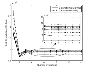
Figure 1: Convergence of the proposed solution where the number of CUEs and D2D UEs served by each relay node is $5$ and $3$, receptively (e.g., $|\mathcal{U}_{l}|=8$). $D_{r,d}$ and $D_{d,d}$ are set to $50~{}{\rm m}$, and uncertainty in CQI parameters is assumed to be not more than $25\%$.

VIII-B1 Convergence and goodness of the solution

In Fig. 1, we show the convergence behavior of our proposed distributed algorithm. In particular, we plot the average achievable data rate for the UEs in different network realizations versus the number of iterations. The algorithm starts with uniform power allocation over RBs, which provides a higher data rate at the first iteration; however, it may cause severe interference to other receiving nodes. As the algorithm executes, the allocations of RB and power are updated considering the interference threshold and data rate constraints. From this figure it can be observed that the solution converges to a stable data rate very quickly (e.g., in less than $10$ iterations).

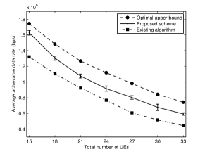
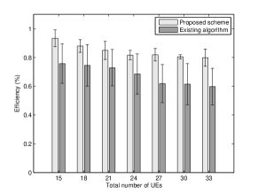
Figure 2: (a) Average achievable data rate for optimal upper bound, distributed stable matching and existing algorithm. (b) Efficiency of the proposed solution and the existing algorithm. Total number of UEs (i.e., $C+D$) are varied from $9+6=15$ to $15+18=33$. $D_{r,d}$ and $D_{d,d}$ are assumed to be $50~{}{\rm m}$.

We compare the performance of our proposed scheme with a dual-decomposition based suboptimal resource allocation scheme proposed in [43]. We refer to this scheme as existing algorithm. In this scheme, the relay node allocates RBs considering the data rate requirement and the transmit power is updated in an iterative manner by updating the Lagrange dual variables. For details refer to [43, Algorithm 2]. The complexity of this algorithm is of $\mathcal{O}\left(NU_{l}\log N+N\log U_{l}+\Delta\right)$, where $\Delta$ denotes the number of iterations it takes for the power allocation vector to converge [43].

In Fig. 2, we show the performances of the proposed distributed scheme and the existing algorithm, and the upper bound of the optimal solution which can be obtained in a centralized manner using Algorithm 1. We use the MATLAB optimization toolbox to obtain this upper bound. We plot the average achievable data rate for the UEs versus the total number of UEs. The average data rate is given by $R_{\rm avg}=\frac{\displaystyle\sum_{u\in\{\mathcal{C}\cup\mathcal{D}\}}R_{u}^{\rm ach}}{C+D}$, where $R_{u}^{\rm ach}$ is the achievable data rate for UE $u$. Note that, for a given number of RBs, increasing the number of UEs decreases the data rate. Recall that, the complexity of both the proposed and reference schemes is linear with the number of RBs and UEs; and for the optimal solution, the complexity is cubic to the number of RBs and UEs. As can be seen from this figure, the proposed approach outperforms the existing algorithm and performs close to the optimal solution.

In order to obtain more insights into the performance, in Fig 2, we plot the efficiency of the proposed scheme and existing algorithm for different number of UEs. Similar to [44, Chapter 3], we measure the efficiency as $\eta_{(\cdot)}=\frac{R_{(\cdot)}}{R_{\rm optm}}$, where $R_{\rm optm}$ is the network sum-rate for optimal solution. The parameters $R_{\rm prop}$ and $R_{\rm exst}$ denote the data rate for the proposed and existing schemes, respectively, which are used to calculate the corresponding efficiency metric $\eta_{\rm prop}$ and $\eta_{\rm exst}$. The closer the value of $\eta_{(\cdot)}$ to $1$, the nearer the solution is to the optimal solution. Clearly, the efficiency of the existing algorithm is lower compared to the proposed scheme. From the figure we observe that even in a dense network scenario (i.e., $C+D=15+18=33$) the proposed scheme performs $80\%$ close to the optimal solution (compared to $60\%$ for the existing algorithm); however, with much less computational complexity.

VIII-B2 Impact of relaying

We compare the performance of the proposed method for relay-aided D2D communication with a conventional underlay D2D communication scheme. In this scheme[6], an RB allocated to CUE can be shared with at most one D2D link. The D2D UEs share the same RB(s) (allocated to a CUE using Algorithm 3) and communicate directly with their peers without a relay if the data rate requirements for both the CUEs and D2D UEs are satisfied; otherwise, the D2D UEs refrain from transmitting. We refer to this underlay D2D communication scheme [6] as the reference scheme. Notice that this conventional (e.g., direct) D2D communication approach can save half of the RBs. Therefore, as mentioned in footnote 3, data rate of $u_{l}$ in the reference scheme is given by $R_{u_{l}}^{\rm ref}=\sum\limits_{n=1}^{N}x_{u_{l}}^{(n)}B_{RB}\log_{2}\left(1+P_{u_{l}}^{(n)}\tilde{\gamma}_{u_{l}}^{(n)}\right)$. On the contrary, data rate of $u_{l}$ in the proposed relay-aided approach is given by $R_{u_{l}}^{\rm prop}=\sum\limits_{n=1}^{N}\tfrac{1}{2}x_{u_{l}}^{(n)}B_{RB}\log_{2}\left(1+P_{u_{l},l}^{(n)}\gamma_{u_{l},l,1}^{(n)}\right)$.

1. Average achievable data rate vs. distance between D2D UEs: The average achievable data rates of D2D UEs for both the proposed and reference schemes are illustrated in Fig. 3. Although the reference scheme outperforms when the distance between the D2D UEs is small (i.e., $d<40~{}\text{m}$), our proposed approach, which uses relays for D2D traffic, can greatly improve the data rate especially when the distance increases. This is due to the fact that when the distance increases, the performance of direct communication deteriorates due to increased signal attenuation. Besides, when the D2D UEs share resources with only one CUE, the spectrum may not be utilized efficiently, and therefore, the achievable rate decreases. As a result, the gap between the achievable rate with our proposed algorithm and that with the reference scheme widens when the distance increases.

2. Gain in aggregate achievable data rate vs. varying distance between D2D UEs: The gain in terms of aggregate achievable data rate under both uncertain and perfect CQI is shown in Fig. 4. We calculate the rate gain as follows: $R_{\rm gain}=\frac{R_{\rm prop}-R_{\rm ref}}{R_{\rm ref}}\times 100\%$, where $R_{\rm prop}$ and $R_{\rm ref}$ denote the aggregate data rate for the D2D UEs in the proposed scheme and the reference scheme, respectively. The figure shows that, compared to direct communication, with the increasing distance between D2D UEs, relaying provides considerable gain in terms of achievable data rate and hence spectrum utilization. As expected, the gain reduces under channel uncertainty since the algorithm becomes cautious against channel fluctuations and allocates RBs and power accordingly to protect the receiving nodes in the network. Note that there is a trade-off between performance gain and robustness against channel uncertainty. For example, when the distance $D_{r,d}=50~{}\text{m}$, the performance gain of relaying under perfect CQI is $30\%$. In the case of uncertain CQI, the gain reduces to $24\%$ and $16\%$ for the uncertainty bound parameter $\xi=0.25$ and $\xi=0.50$, respectively. As the uncertainty bounds increase, the system becomes more roust against uncertainty; however, the achievable data rate degrades.

3. Effect of relay-UE distance and distance between D2D UEs on rate gain: The performance gain in terms of the achievable aggregate data rate under different relay-D2D UE distances is shown in Fig. 5. It is clear from the figure that, even for relatively large relay-D2D UE distances, e.g., $D_{r,d}>60~{}\text{m}$, relaying D2D traffic provides considerable rate gain for distant D2D UEs.

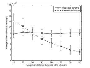
Figure 3: Gain in average achievable data rate with varying distance between D2D peers using a setup similar to that for Fig. 1. The reference scheme is an underlay D2D communication approach proposed in [6].

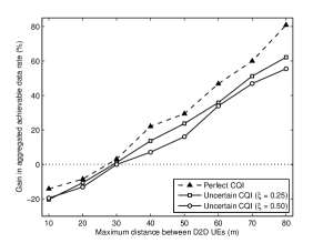
Figure 4: Gain in aggregate achievable data rate for both perfect and uncertain CQI parameters. For uncertain CQI, uncertainty bound $\xi=0.25$ and $\xi=0.50$ mean that uncertainty in CQI parameters is not more than $25\%$ and $50\%$, respectively. For both the perfect and uncertain cases, there is a critical distance beyond which relaying of D2D traffic provides significant performance gain.

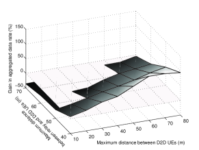
Figure 5: Effect of relay distance on rate gain: $|\mathcal{C}|=15$, $|\mathcal{D}|=9$. Uncertainty in CQI parameters is assumed to be not more than $25\%$. For every $D_{r,d}$, there is a distance threshold (i.e., upper position of the light-shaded surface) beyond which relaying provides significant gain in terms of aggregate achievable rate.

IX Conclusion

We have investigated the radio resource allocation problem in a relay-aided D2D network considering uncertainties in wireless channels and provided an iterative distributed solution to this problem using stable matching. We have analyzed the stability, uniqueness, and optimality of the proposed solution. We have also analyzed the complexity of the proposed approach. Numerical results have shown that the distributed solution is close to the centralized optimal solution with significantly lower computational complexity. We have compared the proposed relay-aided D2D communication scheme with an underlay D2D communication scheme. As an extension of this work, design and analysis of a unified mdium access control (MAC) protocol incorporating mode selection, device discovery, and such relay-aided D2D communication in the context of LTE-A network will be worth investigating.

-A Proof of Proposition 2

Note that any arbitrary matching is not necessarily stable. In the following, we show that for any given preference profiles, each iteration of Algorithm 3 ends up with a stable matching (i.e., there is no blocking pair). We prove the proposition by contradiction. Let $\mu_{l}$ be a matching obtained by Algorithm 2 at any step $t$ of Algorithm 3. Let us assume that RB $n$ is not allocated to UE $u_{l}$, but it has a higher order in the preference list. According to this assumption, the $(u_{l},n)$ pair will block $\mu_{l}$.

Since the position of $u_{l}$ in the preference profile of $n$ is higher compared to the user $\hat{u}_{l}$ that is matched by $\mu_{l}$, i.e., $u_{l}\succeq\mu_{l}(n)$, RB $n$ must select $u_{l}$ before the algorithm terminates. However, the pair $(u_{l},n)$ does not match each other in the matching outcome $\mu_{l}$. This implies that $u_{l}$ rejects $n$ (e.g., line $7$ in Algorithm 2) and $(\hat{u}_{l},n)$ is a better assignment. As a result, the pair $(u_{l},n)$ will not block $\mu_{l}$, which contradicts our assumption. Consequently, the matching outcome $\mu_{l}$ leads to a stable matching since no blocking pair exists and the proof concludes.

-B Proof of Proposition 3

The proof is followed by the induction of number of users $U_{l}$, that are supported by relay $l$. For instance, let $\kappa_{u_{l}}=1,~{}\forall u_{l}\in\mathcal{U}_{l}$ (the proof for $\kappa_{u_{l}}>1$ can be done analogously introducing dummy rows [i.e., UEs] in the utility matrix). The basis (i.e., $U_{l}=1$) is trivial, since the only user definitely gets the best RBs according to her preference. When $U_{l}\geq 2$, let us consider $R_{i}^{(j)}$ to be the maximal entity of the utility matrix $\mathfrak{U}_{l}$. For instance, let the matrix $\widehat{\mathfrak{U}}_{l}$ be obtained by removing the $i$-th row and $j$-th column from the utility matrix $\mathfrak{U}_{l}$. If $\mu_{l}$ is a stable matching for $\mathfrak{U}_{l}$, then by definition $\mu_{l}(i)=j$ and hence $\mu_{l}\setminus\{(i,j)\}$ must be a stable matching for $\widehat{\mathfrak{U}}_{l}$. By induction, there exists a unique stable matching $\widehat{\mu}_{l}$ for the smaller matrix $\widehat{\mathfrak{U}}_{l}$. Therefore, the proof is concluded due to the fact that $\mu_{l}=\widehat{\mu}_{l}\cup\{(i,j)\}$ is the unique stable matching for the utility matrix $\mathfrak{U}_{l}$.

-C Proof of Proposition 4

Without loss of generality, let $\mathfrak{R}_{u_{l},l}(\mu_{l})$ denote the data rate achieved by UE $u_{l}$ for any matching $\mu_{l}$ for given uncertainty bounds and $\mathfrak{R}_{l}(\mu_{l})=\displaystyle\sum_{u_{l}\in\mathcal{U}_{l}}\mathfrak{R}_{u_{l},l}(\mu_{l})$ is the sum-rate of all UEs. On the contrary, let $\widehat{\mu}_{l}$ denote an arbitrary unstable outcome better than $\mu_{l}$, i.e., $\widehat{\mu}_{l}$ can achieve a better sum-rate. There are two cases that make $\widehat{\mu}_{l}$ unstable: 1) lack of individual rationality, and/or 2) blocked by a UE-RB pair [5]. We analyze both the cases below.

Case 1 (lack of individual rationality): If RB $n$ is not individually rational, then the utility of $n$ can be improved by removing user $\widehat{\mu}_{l}(n)$ with any arbitrarily user $u_{l}=\mu_{l}(n)$. Hence, the utility of $u_{l}$ increases and $\mathfrak{R}_{u_{l},l}(\widehat{\mu}_{l})<\mathfrak{R}_{u_{l},l}(\mu_{l})$.

Case 2 ($\widehat{\mu}_{l}$ is blocked): When $\widehat{\mu}_{l}$ is blocked by any UE-RB pair $(u_{l},n)$, RB $n$ strictly prefers UE $u_{l}$ to $\widehat{\mu}_{l}(n)$ and one of the following conditions must be true:

(i) $u_{l}$ strictly prefers $n$ to some $\hat{n}\in\widehat{\mu}_{l}(u_{l})$, or

(ii) $\overline{\overline{\widehat{\mu}_{l}(u_{l})}}<\kappa_{u_{l}}$ and $n$ is acceptable to $u_{l}$.

If condition (i) is true, we can obtain a stable matching $\mu_{l}$ by interchanging $n$ and $\hat{n}$ for $u_{l}$ as follows:

$$\mu_{l}(u_{l})=\left\{\widehat{\mu}_{l}(u_{l})\setminus\hat{n}\right\}\cup n.$$ (.1)

Hence, the new data rate of UE $u_{l}$ is

$$\mathfrak{R}_{u_{l},l}(\mu_{l}) =\sum_{j\in\mu_{l}(u_{l})}R_{u_{l}}^{(j)}=R_{u_{l}}^{(n)}+\sum_{\begin{subarray}{c}j\in\mu_{l}(u_{l}),\\ j\neq n\end{subarray}}R_{u_{l}}^{(j)}$$

$$>R_{u_{l}}^{(\hat{n})}+\sum_{\begin{subarray}{c}j\in\widehat{\mu}_{l}(u_{l}),\\ j\neq n\end{subarray}}R_{u_{l}}^{(j)}=\sum_{j\in\widehat{\mu}_{l}(u_{l})}R_{u_{l}}^{(j)}=\mathfrak{R}_{u_{l},l}(\widehat{\mu}_{l})$$ (.2)

where $R_{u_{l}}^{(n)}$ is given by (45). Since $u_{l}$ strictly prefers RB $n$ to $\hat{n}$ and the data rates for other UEs remain unchanged, for condition (i), it can be shown that $\mathfrak{R}_{l}(\mu_{l})\geq\mathfrak{R}_{l}(\widehat{\mu}_{l})$.

When condition (ii) is true,

$$\mathfrak{R}_{u_{l},l}(\mu_{l}) =\sum_{j\in\widehat{\mu}_{l}(u_{l})}R_{u_{l}}^{(j)}+R_{u_{l}}^{(n)}$$

$$>\sum_{j\in\widehat{\mu}_{l}(u_{l})}R_{u_{l}}^{(j)}=\mathfrak{R}_{u_{l},l}(\widehat{\mu}_{l}).$$ (.3)

Let $\hat{u}_{l}=\widehat{\mu}_{l}(n)$ with data rate $R_{\hat{u}_{l}}^{(n)}$. Then

$$\mathfrak{R}_{\hat{u}_{l},l}(\mu_{l}) =\sum_{j\in\widehat{\mu}_{l}(\hat{u}_{l})}R_{\hat{u}_{l}}^{(j)}-R_{\hat{u}_{l}}^{(n)}$$

$$<\sum_{j\in\widehat{\mu}_{l}(\hat{u}_{l})}R_{\hat{u}_{l}}^{(j)}=\mathfrak{R}_{\hat{u}_{l},l}(\widehat{\mu}_{l}).$$ (.4)

From (-C) and (-C), neither $\mathfrak{R}_{l}(\mu_{l})>\mathfrak{R}_{l}(\widehat{\mu}_{l})$ nor $\mathfrak{R}_{l}(\widehat{\mu}_{l})>\mathfrak{R}_{l}(\mu_{l})$. Since for both cases 1) and 2) there is no outcome $\widehat{\mu}_{l}$ better than $\mu_{l}$, by Definition 6, $\mu_{l}$ is an optimal allocation and the proof follows.

References

- [1] M. Hasan and E. Hossain, “Resource allocation for network-integrated device-to-device communications using smart relays,” in IEEE Global Communications Conference Workshops (GC Wkshps), 2013, pp. 597–602.
- [2] M. Hasan, E. Hossain, and D. I. Kim, “Resource allocation under channel uncertainties for relay-aided device-to-device communication underlaying LTE-A cellular networks,” IEEE Transactions on Wireless Communications, vol. 13, no. 4, pp. 2322–2338, April 2014.
- [3] D. I. Kim, W. Choi, H. Seo, and B.-H. Kim, “Partial information relaying and relaying in 3GPP LTE,” in Cooperative Cellular Wireless Networks. Cambridge University Press, 2011.
- [4] Y. Gu, W. Saad, M. Bennis, M. Debbah, and Z. Han, “Matching theory for future wireless networks: fundamentals and applications,” arXiv preprint arXiv:1410.6513, 2014.
- [5] E. Jorswieck, “Stable matchings for resource allocation in wireless networks,” in 17th International Conference on Digital Signal Processing (DSP), July 2011, pp. 1–8.
- [6] M. Zulhasnine, C. Huang, and A. Srinivasan, “Efficient resource allocation for device-to-device communication underlaying LTE network,” in IEEE 6th International Conference on Wireless and Mobile Computing, Networking and Communications (WiMob), 2010, pp. 368–375.
- [7] P. Phunchongharn, E. Hossain, and D. Kim, “Resource allocation for device-to-device communications underlaying LTE-advanced networks,” IEEE Wireless Communications, vol. 20, no. 4, pp. 91–100, 2013.
- [8] Y. Pei and Y.-C. Liang, “Resource allocation for device-to-device communications overlaying two-way cellular networks,” IEEE Transactions on Wireless Communications, vol. 12, no. 7, pp. 3611–3621, 2013.
- [9] R. Zhang, X. Cheng, L. Yang, and B. Jiao, “Interference-aware graph based resource sharing for device-to-device communications underlaying cellular networks,” in IEEE Wireless Communications and Networking Conference (WCNC), 2013, pp. 140–145.
- [10] L. B. Le, “Fair resource allocation for device-to-device communications in wireless cellular networks,” in IEEE Global Communications Conference (GLOBECOM), 2012, pp. 5451–5456.
- [11] L. Su, Y. Ji, P. Wang, and F. Liu, “Resource allocation using particle swarm optimization for D2D communication underlay of cellular networks,” in IEEE Wireless Communications and Networking Conference (WCNC), 2013, pp. 129–133.
- [12] X. Ma, R. Yin, G. Yu, and Z. Zhang, “A distributed relay selection method for relay assisted device-to-device communication system,” in IEEE 23rd International Symposium on Personal Indoor and Mobile Radio Communications (PIMRC), Sept 2012, pp. 1020–1024.
- [13] D. Lee, S.-I. Kim, J. Lee, and J. Heo, “Performance of multihop decode-and-forward relaying assisted device-to-device communication underlaying cellular networks,” in International Symposium on Information Theory and its Applications (ISITA), 2012, pp. 455–459.
- [14] K. Vanganuru, S. Ferrante, and G. Sternberg, “System capacity and coverage of a cellular network with D2D mobile relays,” in IEEE Military Communications Conference (MILCOM), 2012, pp. 1–6.
- [15] C. An, L. Zhang, and W. Liu, “A spectrum allocation algorithm based on matching game,” in 5th International Conference on Wireless Communications, Networking and Mobile Computing (WiCom), Sept 2009, pp. 1–3.
- [16] B. Holfeld, R. Mochaourab, and T. Wirth, “Stable matching for adaptive cross-layer scheduling in the LTE downlink,” in 77th IEEE Vehicular Technology Conference (VTC Spring), June 2013, pp. 1–5.
- [17] X. Feng, G. Sun, X. Gan, F. Yang, X. Tian, X. Wang, and M. Guizani, “Cooperative spectrum sharing in cognitive radio networks: A distributed matching approach,” IEEE Transactions on Communications, 2014.
- [18] O. Semiari, W. Saad, S. Valentin, M. Bennis, and B. Maham, “Matching theory for priority-based cell association in the downlink of wireless small cell networks,” in IEEE 39th International Conference on Acoustics, Speech and Signal Processing (ICASSP), 2014.
- [19] A. El-Hajj, Z. Dawy, and W. Saad, “A stable matching game for joint uplink/downlink resource allocation in OFDMA wireless networks,” in IEEE International Conference on Communications (ICC), June 2012, pp. 5354–5359.
- [20] B. Di, S. Bayat, L. Song, and Y. Li, “Radio resource allocation for full-duplex OFDMA networks using matching theory,” in IEEE Conference on Computer Communications Workshops (INFOCOM WKSHPS), April 2014, pp. 197–198.
- [21] G. Fodor, E. Dahlman, G. Mildh, S. Parkvall, N. Reider, G. Miklós, and Z. Turányi, “Design aspects of network assisted device-to-device communications,” IEEE Communications Magazine, vol. 50, no. 3, pp. 170–177, March 2012.
- [22] M. Sikora, J. Laneman, M. Haenggi, D. Costello, and T. Fuja, “Bandwidth- and power-efficient routing in linear wireless networks,” IEEE Transactions on Information Theory, vol. 52, no. 6, pp. 2624–2633, 2006.
- [23] Alcatel-Lucent, “The LTE network architecture,” December 2009, White Paper.
- [24] A. Abdelnasser and E. Hossain, “Joint subchannel and power allocation in two-tier OFDMA HetNets with clustered femtocells,” in IEEE International Conference on Communications (ICC), June 2013, pp. 6002–6007.
- [25] Z. Shen, J. Andrews, and B. Evans, “Adaptive resource allocation in multiuser OFDM systems with proportional rate constraints,” IEEE Transactions on Wireless Communications, vol. 4, no. 6, pp. 2726–2737, 2005.
- [26] M. Tao, Y.-C. Liang, and F. Zhang, “Resource allocation for delay differentiated traffic in multiuser OFDM systems,” IEEE Transactions on Wireless Communications, vol. 7, no. 6, pp. 2190–2201, 2008.
- [27] S. Boyd and L. Vandenberghe, Convex Optimization. New York, NY, USA: Cambridge University Press, 2004.
- [28] W. Yu and R. Lui, “Dual methods for nonconvex spectrum optimization of multicarrier systems,” IEEE Transactions on Communications, vol. 54, no. 7, pp. 1310–1322, 2006.
- [29] K. Yang, Y. Wu, J. Huang, X. Wang, and S. Verdu, “Distributed robust optimization for communication networks,” in IEEE Conference on Computer Communications (INFOCOM), April 2008.
- [30] S. Sun, W. Ni, and Y. Zhu, “Robust power control in cognitive radio networks: A distributed way,” in IEEE International Conference on Communications (ICC), June 2011, pp. 1–6.
- [31] A. J. G. Anandkumar, A. Anandkumar, S. Lambotharan, and J. Chambers, “Robust rate-maximization game under bounded channel uncertainty,” in IEEE International Conference on Acoustics Speech and Signal Processing (ICASSP), March 2010, pp. 3158–3161.
- [32] R. Hettich and K. O. Kortanek, “Semi-infinite programming: theory, methods, and applications,” SIAM review, vol. 35, no. 3, pp. 380–429, 1993.
- [33] S. S. Dragomir, “A survey on Cauchy-Bunyakovsky-Schwarz type discrete inequalities,” Journal of Inequalities in Pure and Applied Mathematics, vol. 4, no. 3, pp. 1–142, 2003.
- [34] D. Gale and L. S. Shapley, “College admissions and the stability of marriage,” American Mathematical Monthly, pp. 9–15, 1962.
- [35] B. Rastegari, A. Condon, N. Immorlica, and K. Leyton-Brown, “Two-sided matching with partial information,” in 14th ACM Conference on Electronic Commerce. New York, NY, USA: ACM, 2013, pp. 733–750.
- [36] A. B. MacKenzie and L. A. DaSilva, “Game theory for wireless engineers,” Synthesis Lectures on Communications, vol. 1, no. 1, pp. 1–86, 2006.
- [37] G. O’Malley, “Algorithmic aspects of stable matching problems,” Ph.D. dissertation, University of Glasgow, 2007.
- [38] F. Berggren, R. Jantti, and S.-L. Kim, “A generalized algorithm for constrained power control with capability of temporary removal,” IEEE Transactions on Vehicular Technology, vol. 50, no. 6, pp. 1604–1612, 2001.
- [39] S. Im, H. Jeon, and H. Lee, “Autonomous distributed power control for cognitive radio networks,” in IEEE 68th Vehicular Technology Conference (VTC-Fall), 2008, pp. 1–5.
- [40] 3GPP TS 36.321 V12.1.0, “Medium Access Control (MAC) protocol specification (release 12),” 3rd Generation Partnership Project (3GPP), Tech. Rep., March 2014.
- [41] A. E. Roth and M. A. O. Sotomayor, Two-Sided Matching: A Study in Game-theoretic Modeling and Analysis. Cambridge University Press, 1992, no. 18.
- [42] B. Kaufman and B. Aazhang, “Cellular networks with an overlaid device to device network,” in 42nd Asilomar Conference on Signals, Systems and Computers, Oct 2008, pp. 1537–1541.
- [43] H. Zhang, C. Jiang, N. Beaulieu, X. Chu, X. Wen, and M. Tao, “Resource allocation in spectrum-sharing OFDMA femtocells with heterogeneous services,” IEEE Transactions on Communications, vol. 62, no. 7, pp. 2366–2377, July 2014.
- [44] L. Song, Z. Han, and C. Xu, Resource Management for Device-to-Device Underlay Communication. Springer, 2013.