Steady state relativistic stellar dynamics around a massive black hole

Abstract

A massive black hole (MBH) consumes stars whose orbits evolve into the small phase-space volume of unstable orbits, the “loss-cone”, which take them directly into the MBH, or close enough to interact strongly with it. The resulting phenomena: tidal heating and tidal disruption, binary capture and hyper-velocity star ejection, gravitational wave (GW) emission by inspiraling compact remnants, or hydrodynamical interactions with an accretion disk, are of interest as they can produce observable signatures and thereby reveal the existence of the MBH, affect its mass and spin evolution, probe strong gravity, and provide information on stars and gas near the MBH. The continuous loss of stars and the processes that resupply them shape the central stellar distribution. We investigate relativistic stellar dynamics near the loss-cone of a non-spinning MBH in steady-state analytically and by Monte Carlo simulations of the diffusion of the orbital parameters. These take into account Newtonian mass precession due to enclosed stellar mass, in-plane precession due to general relativity, dissipation by GW, uncorrelated two-body relaxation, correlated resonant relaxation (RR) and adiabatic invariance due to secular precession, using a rigorously derived description of correlated post-Newtonian dynamics in the diffusion limit. We argue that general maximal entropy considerations strongly constrain orbital diffusion in steady-state, irrespective of the relaxation mechanism. We identify the exact phase-space separatrix between plunges and inspirals, predict their steady-state rates, and verify they are robust under a wide range of assumptions. We derive the dependence of the rates on the mass of the MBH, show that the contribution of RR is small, and discuss special cases where unquenched RR in restricted volumes of phase-space may affect the steady-state substantially.

1. Introduction

1.1. Background

Strong interactions of stars with a massive black hole (MBH) in a galactic center lead to a variety of extreme phenomena, as well as provide mass for the growth and evolution of the MBH. The small phase-space volume of orbits whose periapse lies close enough to the MBH to lead to a strong interaction is called the loss-cone (Frank & Rees, 1976), since in most cases the interaction destroys the star, either immediately (for example by a direct plunge through the event horizon or by tidal disruption outside it (Rees, 1988) or gradually, after the orbit decays by some dissipation mechanism (for example the emission of gravitational waves (GW) (Hils & Bender, 1995), tidal heating of the star by the MBH (Alexander & Morris, 2003), or drag against a massive accretion disk (Ostriker, 1983)). Even when the star survives the encounter, for example in a tidal scattering event (Alexander & Livio, 2001), the restricted set of orbits that allow such near-misses lie very close to the loss-cone phase-space. Since typically stars do not survive long on loss-cone orbits, the key questions is how, and at what rate are these orbits repopulated by new stars. The stellar dynamical study of this question is known as loss-cone theory. A main re-population channel is by dynamical relaxation mechanisms, which randomize stable orbits and causes them to diffuse in phase-space into the loss-cone. The close interaction event rates in the steady-state of dynamically relaxed systems are of particular interest, both because these can be derived from first principles independently of initial conditions, and because these correspond, statistically, to the cases most likely to be observed.

Studies of the loss-cone can be broadly categorized by four criteria: whether they deal with processes that lead to immediate stellar destruction (infall) or a gradual one (inspiral); whether they are strictly Newtonian or include also general relativity (GR), fully or perturbatively; whether they include only slow non-coherent two-body relaxation (i.e., non-resonant relaxation, NR Chandrasekhar 1944) or also fast coherent relaxation (known as resonant relaxation, RR, Rauch & Tremaine 1996. See Section 2); and finally by the calculation methods employed: whether they are analytical, or based on the diffusion approximation either by direct numerical solutions of the Fokker-Planck (FP) equations or by Monte-Carlo (MC) methods, or whether they employ direct $N$-body simulations.

Early studies focused on the infall rates of tidal disruption events in the Newtonian approximation, using analytic and FP-based methods (Frank & Rees, 1976; Young et al., 1977; Cohn & Kulsrud, 1978; Shapiro & Marchant, 1978). These studies were subsequently updated and generalized to include some deviations from spherical symmetry (Syer & Ulmer 1999; Magorrian & Tremaine 1999; see review by Alexander 2012). The prospects of detecting low-frequency GW from compact remnants spiraling into MBHs (extreme mass ratio inspiral (EMRI) events) with long-baseline space-borne GW detectors (Amaro-Seoane et al., 2007) motivated studies of the inspiral rates for EMRIs in using FP-based methods in the NR-only limit with perturbative GR (Hils & Bender 1995; Sigurdsson & Rees 1997; Miralda-Escudé & Gould 2000; Freitag 2001, 2003; Ivanov 2002; Hopman & Alexander 2005, 2006b; see review by Sigurdsson 2003). The effects of the MBH spin on the EMRI rates were also considered (Amaro-Seoane et al., 2013).

A unifying framework relating plunge and inspiral processes was formulated by Alexander & Hopman (2003) and used to estimate infall and inspiral event rates in the Galactic Center in the NR-only limit: infall by direct plunge and tidal disruption, inspiral by GW emission and tidal heating (Alexander & Morris, 2003), as well as tidal scattering events (Alexander & Livio, 2001). Different attempts to estimate the infall and inspiral rates yielded a wide, uncertain range of values that spans several orders of magnitudes (Sigurdsson, 2003; Alexander, 2012).

Fast relaxation by RR can be effective on the small spatial scales where most EMRIs originate and importantly, where stellar orbits are observed in the Galactic Center and can therefore provide empirical constraints (Hopman & Alexander, 2006a). This realization motivated a re-evaluation of relaxation processes and their impact on dynamics very close to MBHs. An approximate comparison of the relative rates of RR and NR suggested that the branching ratio between plunges and inspirals depends strongly on the efficiency of RR, which was then poorly understood (Hopman & Alexander, 2006a; Eilon et al., 2009). This added a yet larger uncertainty to EMRI rate estimates. A key question is the physical origin and characteristics of the quenching mechanism that perturbs the near-Keplerian symmetry that generates RR, and causes the orbits to drift in phase-space from their initial values.

Initial analysis of RR in the relativistic context (Rauch & Tremaine, 1996) indicated that rapid GR precession on very eccentric orbits likely plays a key role in quenching RR. Importantly, GR quenching can prevent RR from rapidly pushing all stars into plunge orbits, thereby allowing slow inspiral to produce detectable periodic GW signals (EMRIs) (Hopman & Alexander, 2006a). In these earlier studies the deterministic GR precession was treated as an effective stochastic perturbation of the Keplerian orbits.

First indications that the precession cannot be treated that way, and that the long-timescale behavior of RR is not well described as a Markov process (random walk), were uncovered in post-Newtonian small $N$-body simulations of direct plunge and GW inspiral events (Merritt et al., 2011, MAMW11). These revealed oscillatory orbital behavior at high eccentricities that appeared to act as a barrier against further evolution to even higher eccentricities and subsequent infall or inspiral. MAMW11 dubbed this dynamical phenomenon the Schwarzschild Barrier (SB), and showed that the oscillations are well approximated by the simple ansatz of assuming 2-body GR dynamics in the presence of a randomly oriented fixed force vector (Alexander, 2010), representing the residual force due to the background stars. While the effect appeared related to the EMRI-preserving RR quenching predicted by Hopman & Alexander (2006a), its magnitude seemed much stronger than anticipated, in that it not only damped the RR torques, but actually appeared to prevent the orbits from interacting closely with the MBH at all. The larger-scale relativistic $N$-body simulations of Brem et al. (2014, BAS14) confirmed that GR precession quenches RR roughly on the scale of the SB, and concluded that the resulting EMRI rates are consistent with those driven by NR.

The SB phenomenon was subsequently explained rigorously in terms of the adiabatic invariance (AI) of the GR precession against the coherent RR torques, when the precession period is shorter than the typical RR coherence time (the $\boldsymbol{\eta}$-formalism, Bar-Or & Alexander 2014; see review by Alexander 2015). By describing the RR torques due to the background stars in terms of a correlated noise field, it is possible to formulate an effective FP description for RR that takes into account AI, and to derive the corresponding effective diffusion coefficients (DCs), whose form and behavior depends critically on the assumed temporal smoothness of the noise model. The continuous orbital evolution of the stellar background suggests that the physically correct form of the stochastic torques is that of a smooth (infinitely differentiable, $C^{\infty}$) noise. The AI is maximal for smooth noise. In that case its dynamical effect can be described as a faster than exponential suppression of the diffusion coefficients below some critical angular momentum limit. The vanishing phase-space density past this limit grows so slowly ($\sim\log t$), that the limit can be considered as an effective barrier fixed in time. While this limit is not a true barrier, nor a reflecting one, it does effectively divide phase-space into a region where RR can be efficient, and a region where it cannot. As we show below, the presence of the competing process of NR substantially limits the significance of AI in the dynamics of the loss-cone on long timescales (of order of the NR relaxation time).

This study focuses mainly on the implications of NR and RR around a MBH for loss-rates. However, these dynamical processes are also relevant for understanding and modeling other processes around MBHs, and in particular the Galactic MBH, SgrA^⋆. Although the inner Galactic Center contains a relatively small and manageable number of stars by the standards of current Newtonian $N$-body codes, it is still extremely challenging to simulate it directly both because of the extreme dynamical range introduced by the high MBH to star mass ratio, and because of the added complexity of the GR equations of motion. The impact of MBH spin and RR on orbital tests of GR in the Galactic Center were studied with post-Newtonian small $N$-body simulations (Merritt et al., 2010). A study of the implications of RR for the formation mechanisms of the of stars orbiting SgrA^⋆, either resorted to large Newtonian-only $N$-body simulations (Perets et al., 2008), or substantially underestimated the efficiency of AI in quenching RR by using a MC scheme based on the simple fixed force ansatz with non-differentiable ($C^{0}$) noise, to study the implications of the SB for stars in the Galactic Center (Antonini & Merritt, 2013; Antonini, 2014).

1.2. Objectives and overview

The objectives of this study are to integrate the recent insights about the role correlated noise plays in determining the properties of RR and its formulation as an effective diffusion process (Bar-Or & Alexander, 2014) together with the known properties of NR; to derive a rigorous computational framework for calculating the steady-state phase-space density near the relativistic loss-cone and the resulting loss-rates, and to use this framework for a systematic study of the dependence of the results on the various physical mechanisms involved in the dynamics: mass (Newtonian) precession, GR precession, GW dissipation, the RR noise model and coherence time. The ultimate objective is to provide well-defined estimates of the infall and inspiral rates (including, but not limited to direct plunges, tidal disruptions and EMRIs) and their scaling with the properties of the galactic nucleus (MBH mass and stellar density). These can then inform design decisions about planned surveys and experiments, and serve as benchmarks for more detailed future studies.

We focus our study on a simplified galactic nucleus containing a stationary non-spinning (Schwarzschild) MBH surrounded by a Keplerian, spherically symmetric (in the time-averaged sense), power-law cusp of single mass stars (the background cusp). Direct relativistic $N$-body simulations generate, by construction, the correct dynamics, but are presently limited by computational costs to unrealistically small $N$, which generally cannot be scaled up to astrophysically relevant values since different dynamical mechanisms scale differently with $N$ (e.g., Heggie & Hut, 2003). Moreover, they allow little freedom to switch on/off the various physical mechanisms that affect the outcome. It is therefore difficult to disentangle their contributions and interpret the results.

Here we follow a different approach. We represent the evolution of the system in the realistic large-$N$ limit as a superposition of diffusion processes. This enables us to isolate and study the effect of the different dynamical mechanisms, and thereby obtain an analytic description of the system.

We calculate the loss-cone phase-space density and loss-rates by two complementary methods. We show that the diffusion in phase-space is well approximated as a separable process: fast diffusion in angular momentum, superposed on a slow diffusion in energy. We then use this separation of timescales to derive analytically the steady-state properties of the system. We also solve the diffusion in energy and angular momentum phase-space numerically by MC simulations, which are statistics-limited, but have the advantage of flexibility in introducing additional dynamical effects and constraints. We cross-validate these two calculation methods, and also compare the MC results to the $N$-body loss-rates of MAMW11 and BAS14, and reproduce the AI effects of Bar-Or & Alexander (2014) in the absence of NR.

This paper is organized as follows. In Section 2 we review the dynamical process of relaxation near a MBH in a galactic nucleus. We present a unified framework for describing both non-coherent two-body relaxation and coherent resonant relaxation. We discuss the role of secular processes in the emergence of adiabatic invariance in the long-term orbital evolution of the system. In Section 3 we describe the structure and properties of phase-space near the loss-cone, and derive analytic estimates for the steady-state distribution and loss-rates. We start, in Section 3.1, by formulating the diffusion equations which govern the evolution of the system. In Section 3.2 we describe of the diffusion process in terms of the streamlines of the probability flow, which provide a powerful visual representation of the dynamics, and guides us in Sections 3.3–3.4 in solving the steady-state distribution and loss-rates (at this stage, without RR or GW dissipation). In Section 3.5, we show that GW dissipation separates the probability flow into two distinct regions in phase-space: a region where stars can inspiral into the MBH while emitting GWs, and a region where stars plunge directly into it. The inspiral event rate is then calculated exactly by locating the separatrix that demarcates the two regions (Appendix A). Finally, in Section 3.6 we show that RR has only a small impact on the steady-state density and loss-rates, and provide a method to quantify its effect. In Section 4 we present our MC procedure for modeling orbital evolution in phase-space (The MC procedure and the NR DCs that enter it are described in Appendices B and C). In Section 4.1 we validate the description RR and the emergence of AI in angular momentum-only simulations against the analytic results of Bar-Or & Alexander (2014), and show that AI is very efficiently suppressed by NR on long timescales. We also show that over short timescales, AI induces the “Schwarzschild Barrier” phenomenon seen in angular momentum and energy phase-space (Merritt et al., 2011), and demonstrate that this dynamical feature is erased over long timescales. We compare in Section 4.2 the MC code against the small $N$-body loss-rates of Merritt et al. (2011) and Brem et al. (2014), and show that the MC and $N$-body give consistent results (The derivation of steady-state rate estimates from MC simulations is described in Appendix B.3). In Section 5 we explore the robustness of the MC-derived rates under various dynamical approximations and assumptions. In Section 5.1 we estimate the rates for the prototypical target of low-frequency GW, the Galactic Center. In Section 5.2 we derive analytically, and confirm with the MC simulations, the weak scaling of the rates with the MBH mass. We discuss and summarize our results in Section 6. In Section 6.1 we focus on the role of the principle of maximum entropy (Appendix E) as a guiding principle in the derivation of the DCs. We argue that RR typically does not play a major role in the steady-state dynamics of the loss-cone. We illustrate this analysis by presenting a fine-tuned idealized counter-example where RR may substantially affect the loss-rates: the interaction of icy planetesimals with a massive circumnuclear accretion disk. We conclude by discussing the limitations of our analysis in Section 6.2.

2. Relaxation around a massive black hole

We present here an overview of dynamical relaxation around a central MBH, and in particular of resonant relaxation, using two complementary approaches. The first, which is closer to the conventional description of the subject (e.g., Rauch & Tremaine, 1996; Hopman & Alexander, 2006a), serves to introduce the basic terms and ideas, and connect the present work to past studies. The second presents a unified framework for describing the coherent and stochastic aspects of relaxation, using adiabatic invariance as the unifying concept in all forms of relaxation. This connects the present work to recent results on the representation of RR as an effective diffusion process, a key tool used here to investigate loss-cone dynamics in the large-$N$ limit.

2.1. Two-body relaxation

To understand the relation between NR and RR, consider a spherical stellar system composed of stars of mass $M_{\star}$ orbiting a central massive object $M_{\bullet}\gg M_{\star}$, and focus on a test star at radius $r$ from the center, where the local stellar number density is $n_{\star}\left(r\right)$. The average net force exerted on the test star by the $\mathrm{d}N_{\star}\left(<b\right)\sim n_{\star}b^{2}\mathrm{d}b$ background stars in a thin small shell around it with radius $b\ll r$ and width $\mathrm{d}b\ll b$, is zero. However, the Poisson fluctuations in the positions of these $\mathrm{d}N_{\star}$ discrete masses generate a residual force of magnitude $\sqrt{\left\langle F^{2}\right\rangle}\sim\sqrt{\mathrm{d}N_{\star}}GM_{\star}^{2}/b^{2}$. This force persists in direction and magnitude until the stars generating it move substantially. For a random stellar velocity field with dispersion $\sigma^{2}\sim GM_{\bullet}/r$, this coherence time is $T_{c}^{NR}\sim b/\sigma\ll r/\sigma\sim P$, where $P$ is the orbital period. Since $T_{c}^{NR}\ll P$, the net encounter is impulsive—a collision, and so in the case of NR, the coherence time is the collision time. The change in velocity due to the residual force over time $T_{c}^{NR}$ is $\delta v\sim\sqrt{\left\langle F^{2}\right\rangle}T_{c}^{NR}/M_{\star}$. Over times $t>T_{c}^{NR}$, these impulses add non-coherently, and the accumulated change in velocity per unit time is $\left\langle\Delta v^{2}\right\rangle_{t}\sim\left(G^{2}M_{\star}^{2}n_{\star}/\sigma\right)\mathrm{d}b/b$. Integration over all shells from $b_{\min}$ to $b_{\max}<r$ (assuming $n_{\star}$ is constant) yields the NR diffusion timescale $T_{NR}\sim\sigma^{2}/\left\langle\Delta v^{2}\right\rangle_{t}\sim\sigma^{3}/\left(G^{2}M_{\star}^{2}n_{\star}\log\Lambda\right)$ where $\Lambda=b_{\max}/b_{\min}$ is the Coulomb factor. These local changes in the test star’s velocity lead to changes in orbital energy and angular momentum at a rate $\left\langle\Delta E^{2}\right\rangle/E^{2}\sim\left\langle\Delta J^{2}\right\rangle/J_{c}^{2}\sim 1/T_{NR}$, where $J_{c}=\sqrt{GM_{\bullet}a}$ is the circular angular momentum, and $a$ the semi-major axis (sma).

2.2. Resonant Relaxation

In a nearly-symmetric potential where the background orbits are nearly fixed on timescales $T_{c}\gg P$, the test star interacts over a long period of time with the entire phase-averaged background orbits, and not only instantaneously with the segment of the orbit closest to it. That is, the interaction is non-local. As in the NR case, the discrete number of stars on the scale of the test star’s orbit, $N_{\star}\left(<r\right)$, gives rise to random fluctuations in the force on it, $\sqrt{\left\langle F^{2}\right\rangle}\sim\sqrt{N_{\star}\left(<r\right)}GM_{\star}^{2}/r^{2}$, which persist on timescale $T_{c}$. However, unlike in the NR case, here $T_{c}\gg P$, and so the orbital energy is adiabatically conserved (see below) and the residual force affects only the orbital angular momentum.

2.3. A unified description of relaxation

Conventionally, orbital evolution is described by a combination of two distinct classes of processes: stochastic relaxation processes (two-body relaxation) and coherent (secular) processes (RR). Here we present a unified framework (summarized in Table 1) for describing and analyzing all the dynamical processes that drive orbital evolution in terms of short-timescale coherent processes that effectively contribute as stochastic processes on longer timescales.

We begin by considering the case where the test star is statistically indistinguishable from the background stars (this case was the focus of early works on RR, and is recast here in a more general context).

It is instructive to consider the various relaxation processes in the order of their associated coherence times. When two stars interact impulsively (as in the case where the impact parameter $b$ is much smaller than the sma $a$ of the orbit around the MBH), the interaction time is effectively limited to the crossing time of the closest approach. Since during the interaction, the force on the test star is nearly constant, the duration of the interaction (the collision timescale) is the coherence timescale $T_{c}^{NR}\sim b/\sigma$ of two-body relaxation. As long as only interactions with small enough $b<a$ are considered, so that $T_{c}^{NR}<P(a)$, the Hamiltonian cannot be orbit-averaged, and therefore all the orbital elements can change by the interaction.

The treatment of two-body relaxation is based on the approximation $T_{c}^{NR}\to 0$, that is, that the interaction time is shorter than any other relevant timescale in the system, and that individual collisions are uncorrelated. In that limit the process is Markovian (Nelson & Tremaine, 1999; Bar-Or et al., 2013) and can therefore be described as diffusion in phase-space.

Two-body interactions with a large impact parameter $b>a$ (i.e., soft encounters) such that $T_{c}^{NR}\sim b/\sigma>P(a)$ are no longer impulsive. This means they cannot be described as occurring instantaneously and locally between two point particles, and therefore can no longer be described by the standard two-body relaxation formalism. In particular, the interaction is no longer Markovian, since the test star is repeatedly affected by the same perturbing star. Since it can be shown (for energy relaxation, Bar-Or et al. 2013) that these soft two-body encounters do not contribute much to the total relaxation, an approximate cutoff on the maximal impact parameter is introduced via the Coulomb logarithm term.

Two-body interactions in the extreme soft limit can be described in terms of an effective diffusion process (Bar-Or & Alexander, 2014). Since $T_{c}>P$, the Hamiltonian can be double-averaged over both the orbit of the test star and the orbits of the background stars. The averaged Hamiltonian is then independent of the mean anomaly, and so the Keplerian energy (semi-major axis) is adiabatically conserved—proof that the contribution of soft collisions to energy relaxation is negligible. The double-averaged Hamiltonian no longer describes point particles, but rather interaction between Keplerian ellipses (“mass wires”), which mutually torque each other and exchange angular momentum, but not energy. Here, the force on a test ellipse by the background ellipses remains constant as long as the orbital orientations of the background ellipses remain fixed (i.e., over the coherence time $T_{c}^{RR}$). In analogy to the case of point-point two-body relaxation, this coherence time can be considered as the interaction (“collision”) time. The coherence time is determined by the fastest process that can reshuffle the background orbital orientations. Since typically the background stars are not on relativistic orbits, the dominant shuffling process is the retrograde in-plane drift of the argument of periapse, $\omega$, due the enclosed stellar mass inside the orbits, on the mass-precession timescale $T_{M}\sim QP/N$ (e.g., Hopman & Alexander, 2006a). As long as there are no competing processes with timescale shorter than $T_{M}$ that could randomize the residual forces of the orbit–orbit interactions, these will torque the orbits and change their angular momentum in a coherent ($\propto t$) fashion. Therefore, the Markovian assumption can used and the diffusion rate is $\left\langle\tau^{2}\right\rangle_{RR}T_{M}\sim QP$. This regime of RR is sometimes called “scalar RR” since it can change the magnitude of the angular momentum as well as its direction.

On timescale substantially longer than the precession period, the Hamiltonian can also be double average over the argument of periapse and the interaction is then between mass annuli (Kocsis & Tremaine, 2015). In this case the collision (coherence) time is the self-decoherencing (or self-quenching) time $T_{c}^{vRR}=T_{sq}\sim J_{c}^{2}/\left\langle\tau^{2}\right\rangle\sim QP/\sqrt{N}$ on which the annuli are re-shuffled by their own mutual torques. The residual torque $\left\langle\tau^{2}\right\rangle_{RR}$ is now also averaged over the argument of periapse, which leads some cancellation of the torques, and therefore $\left\langle\tau^{2}\right\rangle_{vRR}<\left\langle\tau^{2}\right\rangle_{RR}$ and the diffusion rate is $\left\langle\tau^{2}\right\rangle_{vRR}T_{c}^{vRR}\sim QP/\sqrt{N}$. This regime of RR is sometimes called “vector RR” since it can change only the direction of the angular momentum, but not its magnitude. In general, as we consider longer coherence timescales, it becomes possible to average over yet more degrees of freedom (phases), and the averaging results in an effective potential that is yet more symmetric. This in turn reduces the magnitude of the residual forces. It is found that the countervailing effects of smaller torques but longer coherence times lead to faster relaxation $T_{r}\propto v^{2}/\left(\left\langle F^{2}\right\rangle T_{c}\right)$, see Table 1.

We now turn to the case where the timescales of the test-star and the background are different, which was not treated rigorously until recently (Bar-Or & Alexander, 2014), following the discovery in $N$-body simulations (Merritt et al., 2011) of an abrupt transition in phase-space to a different dynamical regime where orbital evolution is governed by deterministic rather than stochastic processes. In this case the precession of the test star is due to the combined prograde GR in-plane precession with period $T_{GR}$ and the retrograde Newtonian precession due to the stellar mass enclosed inside the orbit. Since the GR precession rate $T_{GR}^{-1}$ diverges as $1/j^{2}$, where $j=\sqrt{1-e^{2}}$ and $e$ is the eccentricity, eccentric stars with $j$ smaller than some critical value $j_{0}$ will precess much faster than the background, i.e., $T_{GR}<T_{c}$. In this case, the Hamiltonian can be averaged over both the mean anomaly of the background and of test star, as well as over $\omega$ of the test-star. As a result, the test star’s $j$ is adiabatically conserved. The transition between unconstrained RR-driven diffusion at $j\gg j_{0}$ to strict adiabatic invariance at $j<j_{0}$ was calculated for several models of the effective background “noise” (residual torques) in terms of effective diffusion coefficients by Bar-Or & Alexander (2014), who showed that for a smoothly varying background the transition at $j_{0}$ is extremely sharp, with the $j$-diffusion coefficients suppressed exponentially with the argument $(T_{c}/T_{GR})^{2}\propto(j_{0}/j)^{4}$.

Table 1A unified framework for relaxation processes (see text)

Process	Effective	Averaged quantity	Conserved	Coherence time	Residual force magnitude	Relaxation time
	particles		quantities	$T_{c}$	$\sqrt{\left\langle F^{2}\right\rangle}$	$v^{2}/\left(T_{c}F^{2}\right)$
NR	Points	None	None	$T_{c}^{NR}<P$	$\sim\sqrt{N_{\star}}GM_{\star}\sqrt{Q}/a^{2}$	$\sim Q^{2}P/\left(N\log Q\right)$
RR	Ellipses	Mean anomaly	$E$	$P<T_{c}^{RR}\sim T_{M}<T_{p}$	$\sim\sqrt{N_{\star}}GM_{\star}/a^{2}$	$\sim QP$
vRR	Annuli	Argument of periapse	$E,J$	$T_{p}<T_{c}^{vRR}\sim T_{sq}$	$\sim\sqrt{N_{\star}}GM_{\star}/a^{2}$	$\sim QP/\sqrt{N}$

3. The phase space of the loss-cone

We describe the dynamics of the loss-cone in the Keplerian approximation, where the gravitational potential of the stars is assumed to be negligible relative to that of the central MBH. In that limit, the Keplerian orbital energy is $E=GM_{\bullet}/2a$, where the stellar dynamical convention $E=-E_{\mathrm{true}}>0$ for bound orbits is adopted. The orbital angular momentum is parameterized by $j=J/J_{c}(a)$. We marginalize the dynamics over the orbital angles and consider the evolution in the $(a,j)$ phase-space. We assumes a stationary non-spinning MBH of mass $M_{\bullet}$ that is surrounded by an isotropic power-law cusp of stars of mass $M_{\star}$ each with number density profile $n_{\star}=n_{0}(r/r_{0})^{-\alpha}$. The mass ratio is denoted $Q=M_{\bullet}/M_{\star}$. The cusp is assumed to extend between $a_{\min}$ and $a_{\max}$. The inner boundary at $a_{\min}$ is an absorbing boundary, set at the innermost stable circular orbit. The outer boundary at $a_{\max}$ is the interface to the galaxy around the central cusp, which provides an effectively infinite reservoir of stars to replace those that are lost into the MBH, or evaporate back to the galaxy. The Newtonian gravitational dynamics are described in terms of DCs, whose functional form and normalization are calculated assuming the background cusp and an isotropic distribution of angular momentum. The DCs, together with additional non-Newtonian processes such as an absorbing boundary at the last stable orbit (LSO) and GW dissipation of energy and angular momentum, are then used to generate the dynamics of test particles, and derive their steady-state loss-rates and phase-space density.

Stars reach the MBH by crossing the LSO loss-line in $(a,j)$ phase-space (Figure 1) at $j_{lc}(a)=4/\sqrt{a/r_{g}}$, where $r_{g}=GM_{\bullet}/c^{2}$ (This value of $J_{lc}=J_{c}j_{lc}$ is exact for a zero energy orbit). In addition, it is useful to define in the statistical sense the locus of “no-return” for GW inspiral (EMRI). Conventionally, this is defined by a comparison of timescales as the locus where the time to spiral into the MBH by the emission of GWs, $t_{GW}(a,j)$, is shorter than the time needed to scatter across the LSO line by NR, $(j-j_{lc})^{2}T_{J}(a,j)$, where $T_{J}$ is the $J$-diffusion timescale (Appendix A). Note that the GW timescale line shown in Figure 1 is calculated both using the common simplification $t_{GW}=j^{2}T_{J}$, and with the more accurate form $t_{GW}=(j-j_{lc})^{2}T_{J}$, which yields an arc-like shape that peaks well below the point where the approximate power-law GW line intersects the LSO line. The maximal sma along these lines, $a_{GW}$, is then interpreted as the critical sma for EMRIs, below which phase-space trajectories cannot (statistically) avoid crossing the GW line and becoming EMRIs. The EMRI rate scales as $\propto a_{GW}$ (Eq. (32)). In Section 3.5 and Appendix A we formulate a more rigorous criterion for the GW line by identifying the exact separatrix between phase-space streamlines that plunge directly into the MBH, and those that inspiral into it (see Figure 4). This results in an intermediate value of $a_{GW}$. These three estimates of the GW line are plotted in Figure 1 for reference, and correspond to different EMRI rate predictions. It should be emphasized that the GW line does not enter the MC procedure directly, but is an emergent property. Here we use the separatrix method for analytic rate estimates, which accurately reproduce the MC results (Figure 17).

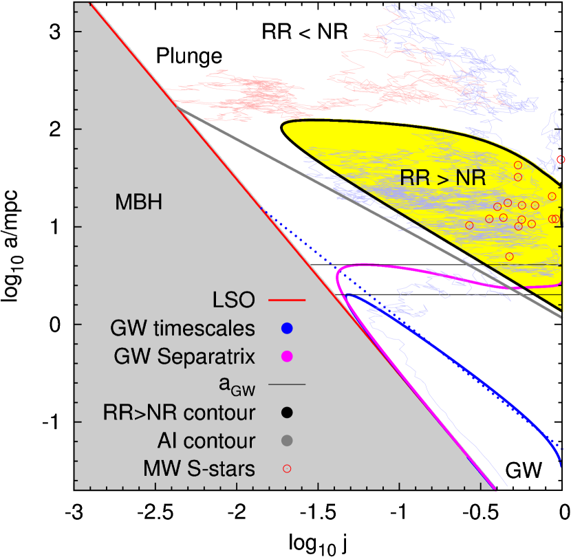
Figure 1.— The $(a,j)$ phase-space of the loss-with the various critical lines and regions, for a model of the Milky Way model with $Q=4\times 10^{6}$, mass-precession coherence time and a Gaussian noise model (Section 5.1). Orbits in the gray area below the LSO line (red) are unstable and promptly plunge into the MBH event horizon (plunge track example in light red line). Where RR diffusion is faster than NR diffusion (yellow region), RR dominates the dynamics. The S-stars observed near the MBH of the MW (red circles) (Gillessen et al., 2009b) lie in the RR dominated region. AI suppresses RR torquing below the AI line (gray). Inside the phase-space region delimited by the GW line (blue), GW dissipation is faster than NR $J$-scattering and orbits spiral into the MBH by the emission of GW (inspiral track example in light blue line). The critical sma for EMRIs, $a_{GW}$ (thin black line), corresponds to the maximum of the GW curve; below it stars become EMRIs before they cross the LSO. The approximate power-law GW line with the often assumed simplification $j_{lc}\to 0$ (dotted blue line), substantially over-estimates $a_{GW}$. The exact separatrix streamline (magenta) provides a more accurate estimate of $a_{GW}$ than either of the timescale-based GW lines.

We derive here analytic estimates for the steady-state distribution and the flux of stars through the loss-cone, quantify the contribution of RR to the loss-rates, and validate our estimates by MC simulations.

3.1. Diffusion equations

On long-enough timescales, where relaxation can be described as a diffusion process (Bar-Or et al., 2013; Bar-Or & Alexander, 2014), the evolution of the probability density function, $n\left(E,J,t\right)$, in ($E$, $J$) phase-space can be describe by an FP equation

$$\frac{\partial n\left(E,J,t\right)}{\partial t} = -\frac{\partial S_{E}\left(E,J,t\right)}{\partial E}-\frac{\partial S_{J}\left(E,J,t\right)}{\partial J}\,,$$ (1)

where the probability current densities in the $E$ and $J$ “directions” are

$$S_{E}\left(E,J,t\right) = D_{E}n\left(E,J,t\right)-\frac{1}{2}\frac{\partial}{\partial E}\left[D_{EE}n\left(E,J,t\right)\right]$$ (2)

$$-\frac{1}{2}\frac{\partial}{\partial J}\left[D_{EJ}n\left(E,J,t\right)\right]\,,$$

and

$$S_{J}\left(E,J,t\right) = D_{J}n\left(E,J,t\right)-\frac{1}{2}\frac{\partial}{\partial J}\left[D_{JJ}n\left(E,J,t\right)\right]$$ (3)

$$-\frac{1}{2}\frac{\partial}{\partial E}\left[D_{EJ}n\left(E,J,t\right)\right]\,,$$

and where $D_{EE}$, $D_{E}$, $D_{JJ}$, $D_{J}$ and $D_{EJ}$ are the DCs that describe the combined effect of NR and RR.

Integrating over $J$ from $J_{lc}$ to $J_{c}$ we obtain the total probability current density gradient (loss-rate) per unit energy

$$\frac{\partial n\left(E,t\right)}{\partial t} = -\int_{J_{lc}}^{J_{c}}\frac{\partial S_{E}}{\partial E}dJ-S_{J}\left(E,J_{c}\right)+S_{J}\left(E,J_{lc}\right)\,,$$

where $n\left(E\right)=\int_{J_{lc}}^{J_{c}}n\left(E,J\right)dJ$ is energy probability density.

It is convenient to transform these expressions to $(E,j)$ since for $j=J/J_{c}$, the current density in the $j$-direction is zero at the boundary ($j=1)$. Generally, under the coordinate change $\mathbf{x}\to\mathbf{x}^{\prime}$ (here $(E,J)\to(E,j)$), the probability density currents, $S_{i}\to S_{i}^{\prime}$, transform as

$$S_{i}^{\prime}\left(\mathbf{x}^{\prime}\right)=\left|\frac{\partial\mathbf{x}}{\partial\mathbf{x}^{\prime}}\right|\frac{\partial x_{i}^{\prime}}{\partial x_{k}}S_{k}\left(\mathbf{x}\right)\,.$$ (5)

Thus

$$S_{j}\left(E,j\right)=S_{J}\left(E,J\right)-j\frac{\partial J_{c}}{\partial E}S_{E}\left(E,J\right)\,,$$ (6)

and since $S_{j}\left(E,j=1\right)=0$, we have

$$\frac{\partial n\left(E,t\right)}{\partial t} = -\int_{J_{lc}}^{J_{c}}\frac{\partial S_{E}}{\partial E}dJ-\frac{\partial J_{c}}{\partial E}S_{E}\left(E,J_{c}\right)+S_{J}\left(E,J_{lc}\right)\,,$$

and

$$\frac{\partial n\left(E,t\right)}{\partial t}=-\frac{\partial}{\partial E}\int_{J_{lc}}^{J_{c}}S_{E}dJ+S_{J}\left(E,J_{lc}\right)\,.$$ (8)

Using Eq. (2) and the fact that $D_{EJ}\left(E,J_{c}\right)=D_{EE}\left(E,J_{c}\right)\partial J_{c}/\partial E$ (Appendix C), allow us to obtain the $J$-averaged FP equation for the energy probability density $n\left(E\right)$,

$$\frac{\partial n(E)}{\partial t} = \frac{1}{2}\frac{\partial^{2}}{\partial E^{2}}\left[\bar{D}_{EE}n\left(E\right)\right]-\frac{\partial}{\partial E}\left[\bar{D}_{E}n\left(E\right)\right]$$ (9)

$$+S_{J}\left(E,J_{lc}\right)\,,$$

in the presence of a loss term $S_{J}\left(E,J_{lc}\right)$, resulting from the flux of stars through the loss-cone, per unit energy, with the $J$-averaged diffusion coefficients

$$\bar{D}_{E}\left(E\right)=n^{-1}(E)\int_{J_{lc}}^{J_{c}}D_{E}\left(E,J\right)n\left(E,J\right)dJ\,,$$ (10)

$$\bar{D}_{EE}\left(E\right)=n^{-1}(E)\int_{J_{lc}}^{J_{c}}D_{EE}\left(E,J\right)n\left(E,J\right)dJ\,.$$ (11)

3.2. Probability flow in phase space

The effects of the various physical mechanisms are more clearly apparent in the flow patterns in phase-space. Since the physical flow is stochastic, it is more useful to describe it in terms of the flow of the probability density. In steady-state, the FP equation (Eq. (1)) can be written as a continuity equation of a compressible flow

$$\frac{\partial}{\partial E}\left[n\left(E,J\right)v_{E}\right]+\frac{\partial}{\partial J}\left[n\left(E,J\right)v_{J}\right]=0\,,$$ (12)

with effective velocities $v_{E}=S_{E}/n\left(E,J\right)$, and $v_{J}=S_{J}/n\left(E,J\right)$. The two-dimensional flow in phase-space $\mathbf{v}=(v_{J},v_{E})$ can be visualized by the streamlines, $v_{J}/dJ=v_{E}/dE$, which are derived below from the steady-state solution of the FP equation (LABEL:eq:EJ_ss).

Using the streamlines, we show in Figures 2–3 the effects of the various physical mechanisms. The probability current densities are determined by the distribution function (DF) of the background stars through the DCs and by DF of the test stars. We begin by assuming that a relaxed cusp will be approximately isotropic (i.e., $f\left(E,J\right)\propto E^{1/4}$) (Bahcall & Wolf, 1976, BW76). The existence of a loss-cone introduces a logarithmic correction, so that the DF is of the form $f\left(E,J\right)\propto E^{1/4}\log\left(J/J_{lc}\right)/\log\left(J_{c}/J_{lc}\right)$ (see Eq. (LABEL:eq:EJ_ss), Figures 6, 7 and Hopman & Alexander 2005). Since the DCs are not strongly affected by this small anisoptropy, it is convenient to assume that the DF of the background is isotropic. Therefore, in the calculation of the streamlines we use a DF of the form $f\left(E,J\right)\propto E^{1/4}$ for the background and a DF of the form $f\left(E,J\right)\propto E^{1/4}\log\left(J/J_{lc}\right)/\log\left(J_{c}/J_{lc}\right)$ for the test stars.

The flow at a point in phase-space is considered $j$-dominated when the streamlines are approximately horizontal (i.e., $\left|\dot{j}\right|/j\gg\left|\dot{a}\right|/a$) and $a$-dominated when the streamlines are approximately vertical (i.e., $\left|\dot{j}\right|/j\ll\left|\dot{a}\right|/a$). As shown in Figures 2–4, the flow is $j$-dominated, apart for two restricted regions in phase-space ($J\to J_{c}$ and the GW-dominated region). Therefore, the full flow field can be separated into two one-dimensional flows, a fact that will be used below to simplify the analytic treatment. Since RR drives stars only in the $j$-direction, this separation is enhanced in the phase-space region where $D_{jj}^{RR}(a,j)>D_{jj}^{NR}(a,j)$, and RR governs the dynamics (see Figures 4–3).

As shown in Figure 3, in the absence of GR precession (i.e., mass precession-only) interior to some sma, RR dominates the dynamics all the way to the loss-cone. In this hypothetical case, the loss rate could be high enough to actually empty the cusp close to the MBH. This would then invalidate the assumption of a single power-low cusp. However, in realty, GR precession does play a crucial role in determining the dynamics and the steady-state. In fact, due to GR precession, RR is totally quenched by the adiabatic invariance (AI) of the angular momentum. This happens for stars with angular momenta below the locus where the precession frequency $\omega_{p}(a,j)=|\omega_{GR}+\omega_{M}|$ equals the coherence frequency $2\pi/T_{c}$, where $\omega_{GR}$ and $\omega_{M}$ are the GR and mass precession frequencies (see AI curve in Figure 4). Only above the AI line can RR be effective. Figure 4 shows a closed contour, somewhat above the AI line, where RR is faster than NR and therefore dominates the dynamics. As we show in Section 3.6, the fact the RR is not effective near the loss-lines means that RR does not play an important role in setting the steady-state and the loss-rates.

Figure 2.— Streamlines of the phase-space flow $\bar{\mathbf{v}}=(\dot{j}/j,\dot{a}/a)$. All dynamical effects apart from resonant relaxation, are included (i.e., two-body relaxation, GW emission, GR precession and mass precession). The DCs are calculated for a Milky Way-like model (isotropic cusp $f\left(E\right)\propto E^{1/4}$ with a MBH of $4\times 10^{6}M_{\odot}$, a mass-ratio of $M_{\bullet}/M_{\star}=5\times 10^{5}$, and total stellar mass $M_{\star}\left(r_{h}\right)=2M_{\bullet}$ where $r_{h}=2\mathrm{pc}$). In addition, the probability current densities are calculated assuming a DF $f\left(E,J\right)\propto E^{1/4}(2J/J_{c}^{2})\log\left(J/J_{lc}\right)/\log\left(J_{c}/J_{lc}\right)$, which is the steady-state solution in the presence of a loss-cone. The color map describes the magnitude of the DCs. The solid cyan line is the GW separatrix. The dashed cyan line indicates the critical sma for EMRIs.

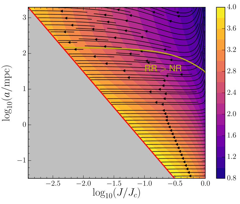
Figure 3.— Streamlines of the phase-space flow $\bar{\mathbf{v}}=(\dot{j}/j,\dot{a}/a)$. All dynamical effects apart from GR precession are included (same cusp model as in Figure 2). In this case RR dominates the dynamics all the way to the loss-cone. Note that this scenario leads to strong depletion of the cusp near the MBH (see for example Figure 15 Bottom). This means that in that region our assumption of a power-law steady-state cusp does not hold. The solid black line marks the region where RR is effective (stronger than NR). The color map describes the strength of the DCs.

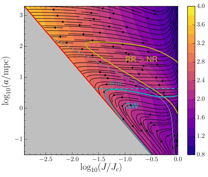
Figure 4.— Streamlines of the phase-space flow $\bar{\mathbf{v}}=(\dot{j}/j,\dot{a}/a)$. All dynamical effects included (same cusp model as in Figure 2). The solid black line marks the region where RR is effective (stronger than NR). The gray line is the locus beyond which RR is totally ineffective due to adiabatic invariance. The color map describes the strength of the DCs. The solid cyan line is the GW separatrix. The dashed cyan line indicates the critical sma for EMRIs.

3.3. Steady state distribution and loss-cone flux

We assume that the system relaxes in $J$ much faster than it relaxes in $E$. This assumption can be justified by noting that $J\in[J_{lc},J_{c}(E)]$ is bound, whereas $E$ is unbound. We therefore assume that the relaxation process is separable: on short timescales stars exchange only angular momentum but not energy and reach their steady-state $J$-distribution at fixed $E$, and only on a much longer timescale do they reach global steady-state in $E$. This assumption of local equilibrium (i.e., in each energy bin the $J$-distribution is relaxed) is further supported by the pattern of the probability current densities (Eqs. (2), (3)) described by the streamlines shown in Figure 5 for the NR-only case. The inclusion of RR only strengthens this separability. This demonstrates that the motion in the $E$-direction (a-direction) occurs only at $j\to 1$, whereas it is almost entirely in the $j$ direction at $j<1$. The validity of this assumption is verified by the excellent match between our analytic predictions and the result of MC simulations, which do not assume separability a-priori, as shown in Figures 6–8. In this section we use this separability assumption and the fluctuation-dissipation relation (Appendix E) to derive the steady-sate state (E,J) distribution and the flux loss-cone flux.

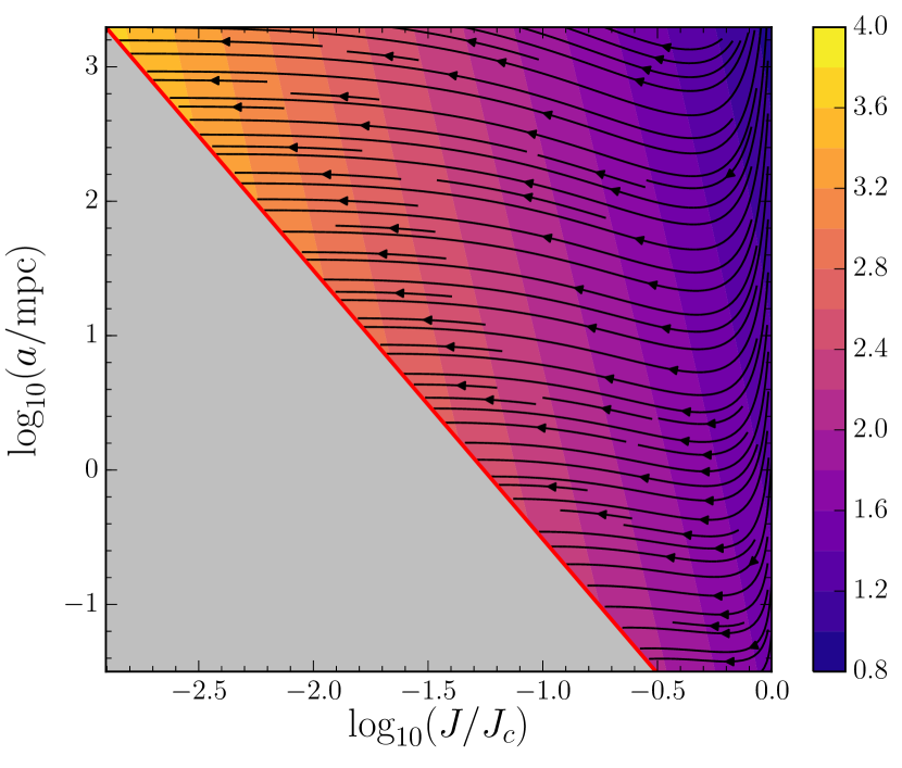
Figure 5.— Streamlines of the phase-space flow $\bar{\mathbf{v}}=(\dot{j}/j,\dot{a}/a)$. Resonant relaxation and GW emissions are not included (same cusp model as in Figure 2). The color map describes the strength of the DCs.

In the limit where there is no energy exchange between stars, the FP equation can written as (Bar-Or & Alexander, 2014)

$$\frac{\partial n(E,J,t)}{\partial t} = \frac{1}{2}\frac{\partial}{\partial J}\left\{JD_{JJ}(E,J)\frac{\partial}{\partial J}\left[\frac{1}{J}n(E,J,t)\right]\right\}$$ (13)

$$= -\frac{\partial S_{J}(E,J,t)}{\partial J}\,,$$

which generally follows from the maximum entropy principle and in fact provides a necessary test for the validity of the DCs (Appendix E). In the absence of a loss-cone (i.e., $J_{lc}\to 0$), the steady-state probability current density $S_{J}\left(E,J,t\right)$ is zero, and the local equilibrium distribution is isotropic

$$n\left(E,J\right)=2J/J_{c}^{2}(E)n(E)\,.$$ (14)

For a finite $J_{lc}$, it follows from the separability assumption, that the probability current density is non-zero and independent of $J$. Therefore, from Eq. (13) we obtain

$$JD_{JJ}(E,J)\frac{\partial}{\partial J}\left[\frac{1}{J}n(E,J,t)\right]=-2S_{J}\left(E\right)\,.$$ (15)

By integrating over $J$ and using the normalization $n\left(E\right)=\int_{J_{lc}}^{J_{c}}n(E,J)dJ$, we obtain

$$S_{J}\left(E\right)=-n\left(E\right)\left/\int_{j_{lc}}^{1}\frac{1-j^{2}}{d_{jj}(E,j)}\frac{dj}{j}\right.\,,$$ (16)

and

$$n\left(E,J\right) = \frac{2J}{J_{c}^{2}}S_{J}\left(E\right)\int_{j_{lc}}^{j}\frac{1}{j^{\prime}d_{jj}(E,j^{\prime})}dj^{\prime},$$ (17)

were $d_{jj}\left(E,j\right)=D_{JJ}\left(E,J\right)/J_{c}^{2}$.

Once the system achieves local equilibrium in $J$ at any $E$ (Eq. (17)), the subsequent steady-state in $E$ is obtained by solving Eq. (9) for $n(E)$, given $S_{J}(E)$,

$$\frac{dR_{P}}{dE}=-S_{J}\left(E\right)=\frac{\partial}{\partial E}\left\{\frac{1}{2}\frac{\partial}{\partial E}\left[\bar{D}_{EE}n\left(E\right)\right]-\bar{D}_{E}n\left(E\right)\right\}\,,$$ (18)

where $R_{p}\left(E\right)=-\int_{J_{lc}}^{J_{c}}S_{E}\left(E,J\right)dJ$, is the cumulative number of stars lost through the loss-cone per unit time. Note that in steady-state, the probability current density in the $J$ direction equals the probability current density gradient in $E$ (from continuity considerations: the density carried by the $J$-current at fixed $E$ and lost through $j_{lc}$ is balanced by the $E$-gradient of the total $E$-current).

3.4. Steady state distribution for two body relaxation

We now show that in the case of two-body relaxation, the solution of the energy FP equation (Eq. (18)) with non-zero flux can be approximated analytically to derive the steady-state density distribution and the plunge rate. Since the plunge rate is small compared to the relaxation rate, the energy distribution asymptotes to the zero-flux (i.e., no plunges) Bahcall & Wolf (1976) power-law solution.

For two-body relaxation, $d_{jj}^{NR}\left(E,j\right)$ asymptotes to a finite value $d_{NR}^{0}\left(E\right)=d_{jj}^{NR}\left(E,j=0\right)$ as $j\to 0$. Since most of the contribution to the current density, $S_{J}\left(E\right)$, reflects the value of $d_{jj}$ at small $j$ (Eq. (16)), it can approximated by $d_{jj}^{0}(E)$, so that

$$S_{J}\left(E\right) \approx -n\left(E\right)\frac{2d_{NR}^{0}(E)}{\log\left(J_{c}^{2}/J_{lc}^{2}\right)-1+J_{lc}^{2}/J_{c}^{2}}$$ (19)

$$\approx -n\left(E\right)\frac{d_{NR}^{0}(E)}{\log\left(J_{c}/J_{lc}\right)}\,,$$

and

$$n\left(E,J\right) \approx n\left(E\right)\frac{2J}{J_{c}^{2}}\frac{\log\left(J^{2}/J_{lc}^{2}\right)}{\log\left(J_{c}^{2}/J_{lc}^{2}\right)-1+j_{lc}^{2}}$$ (20)

$$\approx n\left(E\right)\frac{2J}{J_{c}^{2}}\frac{\log\left(J^{2}/J_{lc}^{2}\right)}{\log\left(J_{c}^{2}/J_{lc}^{2}\right)}\,.$$

Since $d_{jj}^{NR}$ scales as $\bar{D}_{EE}/E^{2}=T_{E}^{-1}$ (Appendix C), it is convenient to represent $S_{J}(E)$ explicitly in terms of the energy relaxation time, $T_{E}$, as $S_{J}(E)=-n\left(E\right)\chi(E)/T_{E}(E)$, where

$$\chi(E) = d_{NR}^{0}(E)/\log\left(J_{c}/J_{lc}\right)=2d_{NR}^{0}(E)/\log\left(E_{lc}/E\right)\,,$$

expresses the logarithmic suppression of the flux due to the decreasing size of the loss-cone away from the MBH, and where $E_{lc}\equiv GM_{\bullet}/32r_{g}$ corresponds to the limit $J_{c}=J_{lc}$ for $J_{lc}=4r_{g}c$ and for Keplerian energy. Note that this is not the true innermost stable circular orbit, but rather a formal extrapolation of the approximations adopted here, used for normalization only. Here we are interested in stars with $E\gg E_{lc}$ where $1/\log\left(E_{lc}/E\right)$ is small. The cumulative plunge rate $R_{P}=-\int S_{J}dE$ can then be approximated as

$$R_{p} \approx \frac{1}{2}N\left(E\right)\frac{\chi\left(E\right)}{T_{E}}+\frac{3}{4}\int_{E}^{E_{\max}}\frac{\chi\left(E^{\prime}\right)}{T_{E}\left(E^{\prime}\right)}N\left(E^{\prime}\right)\frac{dE^{\prime}}{E^{\prime}}\,,$$

where $N\left(E\right)$ is the number of stars with energy larger than $E$.

For an infinite isotropic cusp $n\left(E\right)\propto E^{p-5/2}$ where $0<p<1/2$ (to ensure the DCs are finite), the $J$-averaged DCs are (Bar-Or et al., 2013)

$$\bar{D}_{E} = -\frac{4(1-4p)\log\Lambda}{1+p}\frac{N(E)}{Q^{2}P(E)}E\propto E^{p+1},$$ (23)

$$\bar{D}_{EE} = \frac{16\left(3-2p\right)\log\Lambda}{(1+p)(1-2p)}\frac{N(E)}{Q^{2}P(E)}E^{2}\propto E^{p+2}\,,$$ (24)

and the plunge rate is

$$R_{p}\approx\frac{3-2p}{3-4p}N\left(E\right)\frac{\chi\left(E\right)}{T_{E}}\,.$$ (25)

Since $\chi$ is nearly constant in $E$ for $E\ll E_{lc}$, it can be approximated in that limit by evaluating it at $E_{\min}=GM_{\bullet}/2a_{\max}$. In that case, Eq. (18) has an analytical solution,

$$\frac{\left(4p-3\right)\left(1-4p\right)}{4\left(3-2p\right)}=\chi\,,$$ (26)

which connects the current to the power-law exponent of the cusp. The physical branch of the solution is

$$p = \frac{1}{4}\left(-\sqrt{\chi^{2}+8\chi+1}-\chi+2\right)\approx\frac{1}{4}\left(1-5\chi\right)\,.$$ (27)

Since for $p=1/4$, $d_{jj}^{0}\approx 1/\left(8T_{E}\right)$ (Appendix C), it follows that $\chi\approx 1/\left[8\log\left(1/j_{lc}\right)\right]\ll 1$, and so the Bahcall & Wolf (1976) solution $p=1/4$ (i.e., $\chi\to 0$) is a reasonable approximation in the $E\to E_{\min}$ limit, where $j_{lc}\ll 1$. Thus in steady-state the energy (or sma) distribution is $n\left(E\right)\propto E^{-9/4}$ (or $n\left(a\right)\propto a^{1/4}$). Using Eq. (20) we obtain the ($E,J$) steady-state distribution

$$n\left(E,J\right) \approx \frac{5}{4}N\left(E_{\min}\right)\frac{2J}{J_{c}^{2}}\frac{\log\left(J/J_{lc}\right)}{\log\left(J_{c}/J_{lc}\right)}\left(E/E_{\min}\right)^{-9/4}\,,$$

and a steady-state plunge rate

$$R_{p}\left(a\right) \approx \frac{5}{32}\frac{1}{\log\left(1/j_{lc}\left(a\right)\right)}\frac{N\left(a\right)}{T_{E}\left(a\right)}\,,$$ (29)

where the energy relaxation time is (Bar-Or et al., 2013)

$$T_{E}\left(a\right)=\frac{1}{64}Q^{2}\frac{P\left(a\right)}{N\left(a\right)\log Q}\,.$$ (30)

In the limit $E\to E_{lc}$, $\chi(E)$ can no longer be approximated as fixed nor as small, and the power law solution breaks down. We now argue that this power-law approximation is valid for almost the entire range of MBH masses and their host galactic nuclei. Define $a_{BW}$ as the minimal sma where $\chi$ and $\partial\log\chi/\partial\log E$ are still small enough for this approximation to hold. Since $\partial\log\chi/\partial\log E\propto\chi\propto 1/\log\left(1/j_{lc}\right)$ where $j_{lc}\propto\sqrt{r_{g}/a}$, it follows that $a_{BW}\propto M_{\bullet}$. We are interested to resolve the dynamics close to the MBH in order to obtain a reliable estimate for the EMRI event rate. As we show in Section 3.5, the rate is determined by the dynamics near the critical GW sma, $a_{GW}$. Thus it is sufficient do show that $a_{BW}<a_{GW}$, since then power-law approximation is valid over the entire range of relevant radii. The MC results shown in Figures 6 and 8 for the case of $M_{\bullet}=4\times 10^{6}M_{\odot}$, demonstrate that our analytic estimates (Eqs. (LABEL:eq:EJ_ss), (29)) for the steady-state energy distribution and plunge rate reproduce the simulated results at least down to $a_{GW}$. This holds also for more massive MBHs. The $M/\sigma$ relation and the scalings $a_{BW}\propto M_{\bullet}$ and $a_{GW}\propto\left(\log Q\right)^{-4/5}r_{h}$ (Eq. (A10)) imply $a_{BW}/a_{GW}\propto\left(\log Q\right)^{4/5}M_{\bullet}^{2/\beta}$ and therefore $a_{BW}\lesssim a_{GW}$ up to $M_{\bullet}\sim 10^{9}M_{\odot}$.

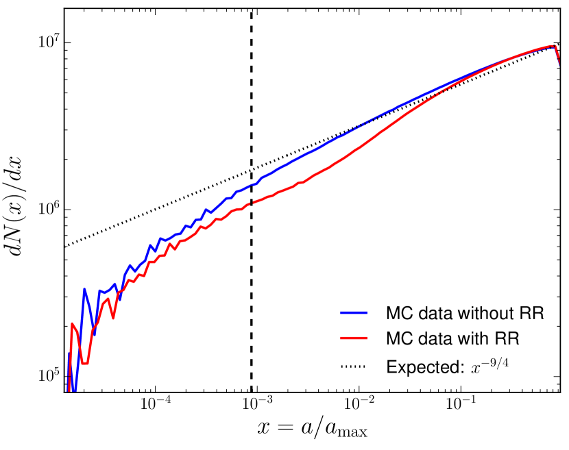
Figure 6.— The energy distribution as function of energy shows a good agreement between the analytic BW76 cusp solution and MC results. The critical sma, $a_{GW}(E_{GW})$ as defined by the sparatrix (see Section 3.5) is shown by a dashed line.

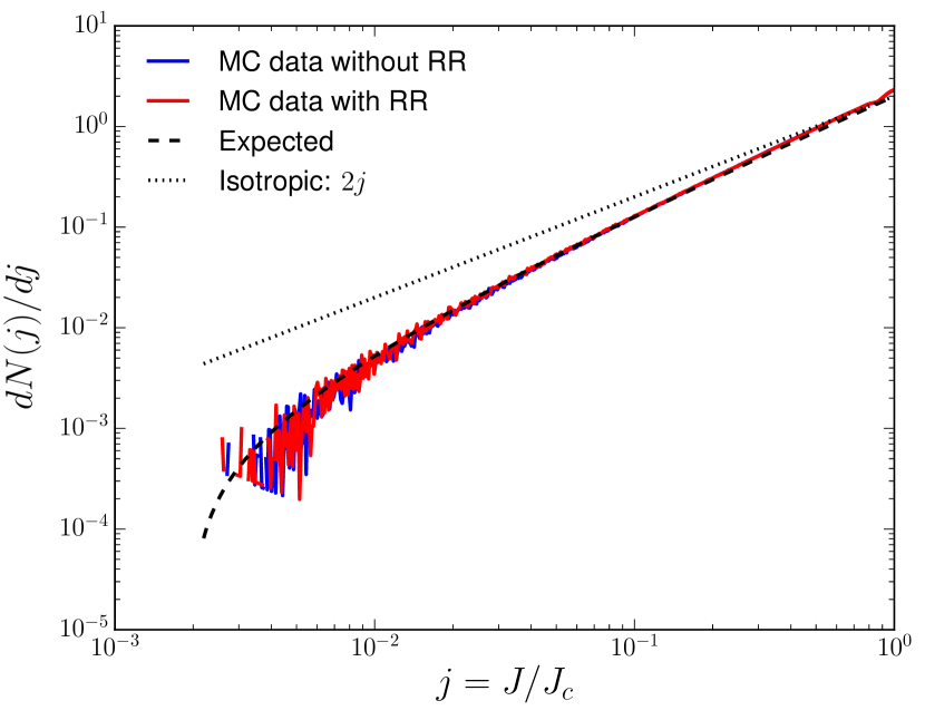
Figure 7.— The angular momentum distribution in a bin centered around $a=0.4a_{\max}$. The MC data shows the expected logarithmically-suppressed distribution (Eq. (LABEL:eq:EJ_ss)) compared with the isotropic one.

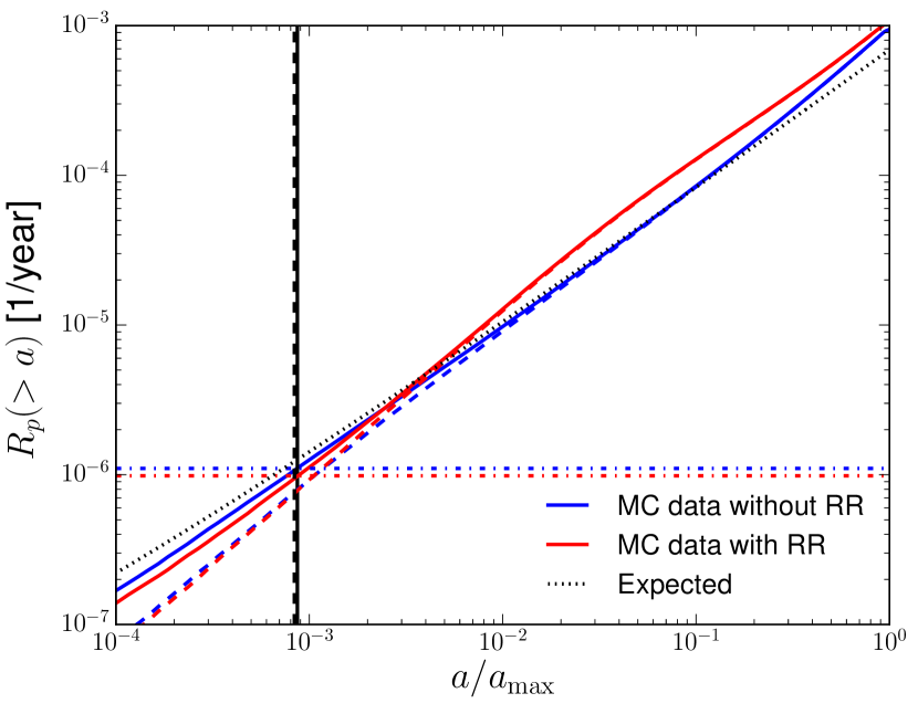
Figure 8.— The plunge rate as a function of semi-major axis. The MC data (without RR) agree with the analytic expression (Eq. (LABEL:eq:RpMW)). The MC results demonstrate that the contribution of RR to the plunge rate is small. The critical sma, $a_{GW}$ (vertical dashed line) as defined by the separatrix (see 3.5) agrees very well with the sma (vertical solid line) where the inspiral rate, $R_{i}^{tot}$ (dash-doted lines), equals the plunge rate $R_{p}^{no\,GW}$ in the absence of GW emission.

3.5. EMRI event rates

So far we ignored the contribution of GW emission to the dynamics. Compact objects can withstand the tidal field of the MBH. When on eccentric orbits, their orbital decay by the emission of GWs can be faster than the diffusion of angular momentum due to the stochastic perturbations of the stellar background. In that case, they inspiral gradually all the way down to the innermost stable circular orbit (ISCO) as EMRIs (Peters & Mathews, 1963; Peters, 1964; Gair et al., 2006), instead of plunging directly into the MBH with $J<J_{lc}$ (Figure 1). The GW signature of plunges and inspirals is very different. The low mass of the compact objects generates weak signals, well below the noise. Plunges result in short, very hard to detect broad spectrum GW flares. In contrast, EMRIs are of special interest since their quasi-periodic signal can be integrated and detected against the noise if the waveform is approximately known.

In the absence of GWs (Figure 5), the streamlines are approximately constant in $a$. In contrast, GW emission diverts the streamlines to tracks that are almost parallel to the loss-cone (i.e., nearly constant $J$) in the phase-space region where GW dominates the dynamics (Figure 2). The outermost inspiraling streamline separates phase-space into two distinct regions. Above this separatrix all streamlines are plunges, while below it all streamlines are inspirals (Figure 4). The continuity equation (Eq. (12)) implies that the probability current in steady-state is constant along a streamline bundle. Since the streamlines in the GW-dominated region below the separatrix originate in phase-space regions where the density is much higher, the small depletion due to EMRI losses is not expected to affect the density at the origin of the streamlines. The EMRI rate can therefore be estimated by identifying the terminal point ($a_{p},j_{lc}$) of the plunge streamline (without GW) corresponding to the separatrix. This is the effective critical sma for EMRIs, $a_{GW}$. The EMRI rate is then obtained by integrating the differential plunge rate in the absence of GW emission from $a_{isco}$ to $a_{GW}$,

$$R_{i}^{tot}=-\int_{E_{GW}}^{E_{isco}}S_{J}\left(E\right)dE=R_{p}\left(a_{GW}\right)\,.$$ (31)

Thus, for a BW76 cusp the EMRI rate is

$$R_{i}^{tot} = \frac{5}{32}\frac{1}{\log\left(1/j_{lc}\left(a_{GW}\right)\right)}\frac{N\left(a_{GW}\right)}{T_{E}\left(a_{GW}\right)}$$ (32)

$$= \frac{a_{GW}}{a_{\max}}\frac{\log\left(1/j_{lc}\left(a_{\max}\right)\right)}{\log\left(1/j_{lc}\left(a_{GW}\right)\right)}R_{p}^{no\,GW}\left(a_{\max}\right)\,,$$

which is approximately linear in $a_{GW}$. The value of $a_{GW}$ is determined by solving the streamline equation $dE/dJ=S_{E}/S_{J}$ with the boundary condition that the streamline trajectory reaches $J_{lc}$ at $E_{\max}$. The probability current densities are estimated by assuming that $S_{J}$ is constant in $J$ and $S_{E}$ results only from GW dissipation. This means that in the absence of GWs, that streamline is constant in $E$ and $a_{GW}$ can be estimated by taking the value of $a$ at $J\gg J_{lc}$. The exact value of $a_{GW}$ depends on the GW emission approximation used and is calculated in Appendix A. As shown in Figure 8, this definition of $a_{GW}$ is indeed a good approximation to the sma where the plunge rate (without GW) is equal to the inspiral rate and can be used to predict the inspiral rate in the MC simulations (Figure 17). As expected, inside $a_{GW}$ the plunge rate with GW decreases relative to the plunge rate without GW (See Figure 9).

Figure 9.— The plunge ratio $R_{p}^{GW}/R_{p}^{no\,GW}$, where $R_{p}^{GW}$ and $R_{p}^{no\,GW}$ are the cumulative plunge rates obtained with and without GW dissipation. The critical sma, $a_{GW}$ (vertical dashed line) as defined by the separatrix (see 3.5) agrees very well with the sma (vertical solid line) where the inspiral rate, $R_{i}^{tot}$, equals the plunge rate $R_{p}^{no\,GW}$ in the absence of GW emission.

3.6. Effect of Resonant Relaxation

Due to the long coherence time, resonant relaxation is a much more effective process than two-body relaxation. However, in regions of phase-space where in-plane GR precession is faster than the coherence time, $j$ becomes an adiabatic invariant and the RR process is quenched. RR it is therefore limited to a small region of phase-space (see Figure 4). The locus where in-plane precession quenches RR by AI (Section 4.1) defines the outer envelope of the region where RR may be efficient relative to NR. The region where RR dominates the dynamics even on long timescales is where by the ratio of the 2nd order DCs exceeds unity, i.e., $D_{jj,RR}/D_{jj,NR}>1$ (See Figure 4). The typical phase-space configuration is shown in Figure 1: the region where RR dominates is detached from the loss-lines; NR is required for the stars to evolve towards them, and therefore the slow NR timescale remains the bottleneck for the loss-rates which are mostly unaffected by RR (see Figure 17). This can be shown formally by re-estimating the probability current density in the presence of RR.

For a smooth noise, the RR diffusion coefficient can be written as (Bar-Or & Alexander, 2014)

$$D_{JJ}^{RR}=2T_{\mathrm{coh}}\nu_{J}^{2}e^{-4\pi j_{0}^{4}/j^{4}},$$ (33)

where $\nu_{J}=\sqrt{\left\langle\tau_{J}^{2}\right\rangle}$ is the residual torque in the $\mathbf{J}$ direction (see Appendix D)

$$\nu_{J}\approx 0.28\sqrt{1-j}\sqrt{N\left(a/2\right)}J_{c}\nu_{R}/Q,$$ (34)

and $j_{0}\left(a\right)$ is the AI locus where the GR precession frequency $\nu_{GR}\left(a,j\right)$ equals to the coherence time

$$j_{0}=\sqrt{2\pi T_{c}\nu_{GR}\left(a,j=1\right)}.$$ (35)

Here we adopt

$$T_{c}=\sqrt{\pi/2}\nu_{p}^{-1}\left(2a,\sqrt{1/2}\right)$$ (36)

where $\nu_{p}$ is the combined mass and GR precession.

The combined diffusion coefficients are

$$D_{J} = D_{J}^{NR}+D_{J}^{RR}\,,$$ (37)

$$D_{JJ} = D_{JJ}^{NR}+D_{JJ}^{RR}\,,$$ (38)

and using Eq. (16), the flux is given by

$$S_{J}\left(E\right)=-n\left(E\right)/\int_{j_{lc}}^{1}\frac{1-j^{2}}{D_{JJ}^{NR}/J_{c}^{2}+D_{JJ}^{RR}/J_{c}^{2}}\frac{dj}{j}\,.$$ (39)

Since $D_{RR}$ is rises up to some maximal value before sharply drops as it approaches $j\to j_{0}$, we can approximate the RR DC as

$$d_{jj}^{RR}\approx\begin{cases}d_{RR}^{0}\left(1-j\right)e^{-4\pi j_{0}^{4}}&j\geq j_{m}\\ 0&j<j_{m}\end{cases}\,,$$ (40)

where $d_{RR}^{0}=2T_{\mathrm{coh}}\nu_{J}^{2}\left(j=0\right)$ and the maximum of $d_{RR}\left(E,j\right)$, occurs at $j_{m}$, given by $j_{m}^{5}/j_{0}^{5}=16\pi\left(1-j_{m}\right)/j_{0}\approx 16\pi\left(1-j_{0}\right)/j_{0}$. The differential flux is therefore given by

$$\frac{S_{J}^{RR}\left(E\right)}{S_{J}^{NR}\left(E\right)} = \left[\int_{j_{lc}}^{j_{m}}\frac{1-j^{2}}{d_{jj}^{NR}}\frac{dj}{j}+\int_{j_{m}}^{1}\frac{1-j^{2}}{d_{jj}^{NR}+d_{jj}^{RR}}\frac{dj}{j}\right]^{-1}$$ (41)

$$\approx \left[1-\frac{\chi_{RR}}{1+\chi_{RR}}\frac{\log\left(16\pi\left(1-j_{0}\right)j_{0}^{4}\right)}{5\log\left(j_{lc}\right)}\right]^{-1}\,,$$

where $\chi_{RR}=d_{RR}^{0}e^{-4\pi j_{0}^{4}}/d_{NR}^{0}$. As shown in Figure 10, this analytic approximation reproduces the MC results.

The small effect of RR on the loss-rates can be estimated by integrating Eq. (41) over the relevant region

$$R_{p}^{RR}\left(E\right)=-\int_{E}^{E_{\max}}S_{J}^{RR}\left(E^{\prime}\right)dE^{\prime}\,.$$ (42)

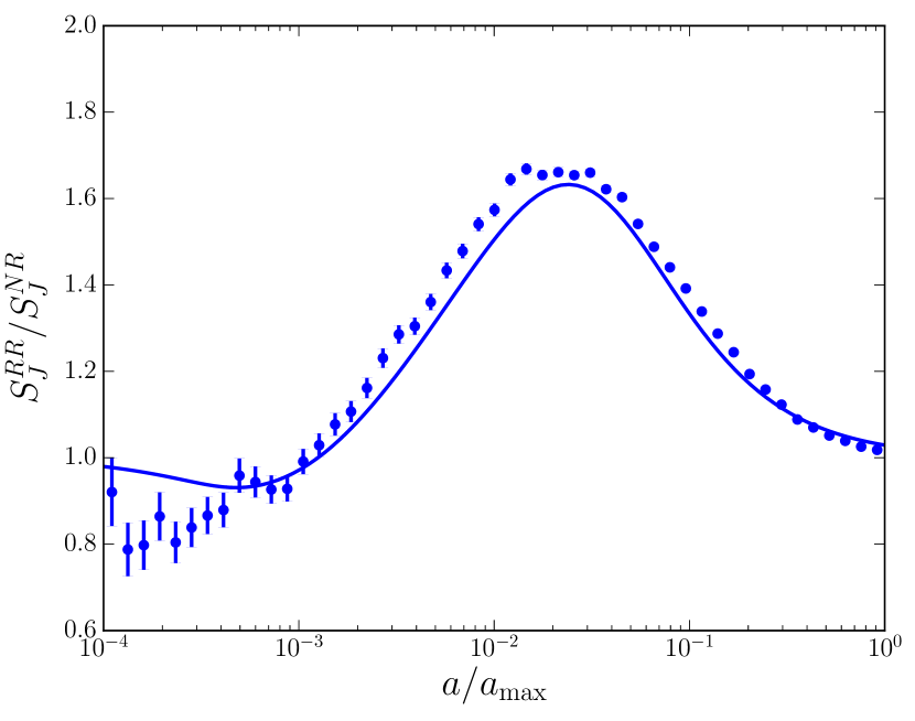
Figure 10.— The ratio between the probability current density in $J$ with and without RR, as function of $a$ (Eq. (41)), which expresses the differential plunge rate. The limited increase in the ratio over its asymptotic value of $1$ in the $a\to 0$ and $a\to\infty$ limits expresses the fact that the contribution of RR to the plunge rate is small.

4. Monte Carlo models

We complement and validate our analytic study of the relativistic loss-cone by numerically evolving the FP equation in both $E$ and $J$ using a MC procedure (described in Appendix B). Unlike the analytic treatment, this procedure does not assume that the evolution in $J$ can be decoupled from that in $E$. The advantages of the MC method over direct $N$-body simulations are the high degree of flexibility it offers for isolating and studying the different mechanisms that affect the dynamics of the loss-cone, the ease of including additional physical effects and of modifying the initial and boundary conditions, and importantly, its scalability to systems with a realistically large number of stars. In Section 5 below we employ the MC procedure to calculate the phase-space density and rates of relaxed galactic nuclei, and in particular, that of a Milky Way-like nucleus with a $4\times 10^{6}\,M_{\odot}$ MBH and $N\sim{\cal O}(10^{7})$ stars on its radius of influence, $r_{h}\sim 2\,\mathrm{pc}$. Such nuclei are considered archetypal for future space-borne missions to detect low-frequency gravitational waves from inspiraling compact objects.

We begin here by validating the MC procedure. We study the dynamics in the restricted case where $E$ remains fixed, which allows a direct test of the impact of adiabatic invariance on the long-term dynamics (Section 4.1). We then compare rate results from our MC procedure in both $E$ and $J$ with the currently available results from direct post-Newtonian $N$-body simulations of small-$N$ ($N<100$) systems (Section 4.2).

4.1. $j$-only Monte Carlo simulations

The maximal entropy limit (Appendix E) provides a basic test for the physical validity of the DCs and of the MC procedure for evolving the Fokker-Planck equation. The probability density of a closed system with zero net angular momentum must asymptote to the maximal entropy solution $\mathrm{d}N/\mathrm{d}j=2j$. Experimentation shows that this is a sensitive test of both the functional form of the DCs and the details of the MC procedure, in particular the implementation of the boundary conditions. We verify the maximal entropy limit in Section 4.1.1. In the absence of NR (for example on timescales $\ll T_{NR}$), a relativistic system that is subject to RR with a smooth background noise should display adiabatic invariance (AI) in the form of a sharp drop in the phase-space density below some small value of $j$ where the GR precession period falls below the coherence time (Bar-Or & Alexander, 2014). RR with non-smooth background noise is not expected to display such an AI barrier (the “Schwarzschild barrier”, Merritt et al. 2011). We demonstrate that our MC procedure reproduces this behavior in Section 4.1.2. Finally, we study the realistic case where NR smears the RR-generated AI in Section 4.1.3, and also show how this smearing appears in the unrestricted case where both $a$ and $j$ evolve.

Since the $j\to 0$ limit is of special interest, it is efficient to use logarithmic bins to collect statistics on the phase-space density. In that case, it is more useful to represent the density as $\mathrm{dN}/\mathrm{d}\log j$,where the maximal entropy solution is $\mathrm{d}N/\mathrm{d}\log j=2j^{2}$ (or $\mathrm{d}N/\mathrm{d}\log_{10}j=2\log(10)j^{2}$).

4.1.1 NR only

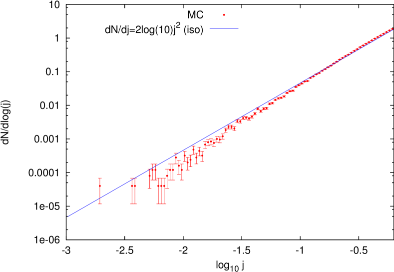
Figure 11.— The convergence of a MC $j$-only NR diffusion simulation to the maximal entropy solution $\mathrm{d}N/\mathrm{d}\log_{10}j=2\ln 10j^{2}$

Figure 11 shows the $j$-PDF at $a=a_{\max}/4$ for an $\alpha=7/4$ cusp with $a_{\max}=10^{4}a_{\min}$, after time $t=100T_{E}$ ($T_{E}=[E^{2}/\Delta(E^{2})]_{a_{\max}}$). Near-complete convergence is already reached at $T\gtrsim T_{E},$ (Section 4.1.3). The convergence to the expected maximal entropy solution is apparent, although a bias toward a somewhat steeper slope for $j\lesssim 0.1$ is observed. In addition to the $\alpha=7/4$ case shown in Figure 11, simulations with other values of $\alpha$ or of $a_{\max}/a_{\min}$ confirm that the maximal entropy solution holds generally.

4.1.2 RR only

Figure 12 shows the $j$-PDF for the RR-only case. The MC code reproduces the AI barrier for smooth noise at $j_{0}=\sqrt{T_{c}\omega_{GR}/2\pi}$ (Bar-Or & Alexander, 2014), while non-smooth noise asymptotes as expected to the maximum entropy solution—a demonstration that this limit does not depend on the nature of the relaxation process.

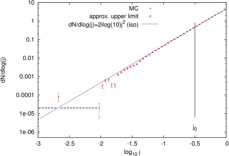
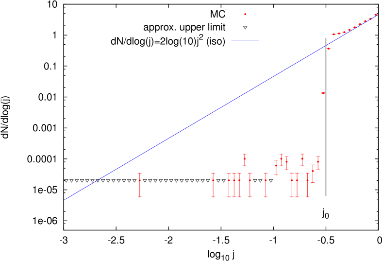
Figure 12.— Adiabatic invariance and the convergence of $j$-RR to the maximal entropy solution $\mathrm{d}N/\mathrm{d}\log_{10}j=2\ln 10j^{2}$ for two different background noise models: non-smooth noise $(C^{0})$ with an exponential ACF (top) and smooth noise ($C^{\infty}$) with a Gaussian ACF (bottom). The predicted characteristic position of the AI front at $j_{0}$ is marked by the vertical line. An approximate upper limit on the density (1 count per bin) was estimated for empty bins (triangles).

4.1.3 NR+RR

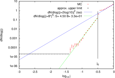
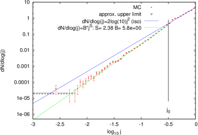
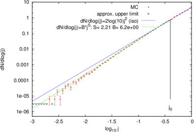
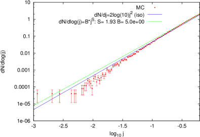
Figure 13.— The suppression of adiabatic invariance by NR and the convergence of $j$-only MC simulations with NR and RR with a Gaussian ACF noise to the maximal entropy solution $\mathrm{d}N/\mathrm{d}\log_{10}j=2\ln 10j^{2}$. All MC runs lasted a fixed time $T_{\mathrm{sim}}=100T_{E}$, were $T_{E}$ is the energy diffusion timescale at $a_{\max}$, but the NR relaxation time was artificially extended to $T_{E}^{\prime}=X_{D}T_{E}$ ($X_{D}\geq 1$) so that $T_{\mathrm{sim}}=(100/X_{D})T_{E}^{\prime}$ (the larger $X_{D}$, the less significant is NR). The predicted characteristic location of the AI barrier at $j_{0}$ is marked by the vertical line. The best fit power-law to the $j$-PDF slope is also shown (green line). An approximate upper limit on the density (1 count per bin) was estimated for empty bins (triangles). Top left: $T_{\mathrm{sim}}=0.1T_{E}^{\prime}$. Top right: $T_{\mathrm{sim}}=T_{E}^{\prime}$. Bottom left: $T_{\mathrm{sim}}=100T_{E}^{\prime}=100T_{E}$. Bottom right: NR-only MC simulation for comparison.

The presence of NR erases the AI cutoff in the $j$-PDF on timescales approaching or exceeding the NR timescale (quantified by the energy diffusion timescale $T_{E}$). This is demonstrated in Figure 13, which shows a sequence of $j$-only MC simulations that include both NR and RR. All the simulation runs had a fixed duration $T_{\mathrm{sim}}=100T_{E}$, which kept the number of binned points, and hence the statistical sampling fluctuations, fixed (the MC values are sampled every $\Delta t=1\,T_{E}$). However, the effective NR timescale was artificially extended to $T_{E}^{\prime}=X_{D}T_{E}$ ($X_{D}\geq 1$), so that $T_{\mathrm{sim}}=(100/X_{D})T_{E}^{\prime}$, and $X_{D}$ was varied from $X_{D}=10^{3}$ ($T_{\mathrm{sim}}=0.1T_{E}^{\prime}$) down to $X_{D}=1$ ($T_{\mathrm{sim}}=100T_{E}^{\prime}$): the larger $X_{D}$, the less significant is NR over $T_{\mathrm{sim}}$. Figure 13 shows results for $T_{\mathrm{sim}}=0.1T_{E}^{\prime}$, $T_{\mathrm{sim}}=T_{E}^{\prime}$, and $T_{\mathrm{sim}}=100T_{E}^{\prime}$. The AI cutoff is substantially smeared already when $T_{\mathrm{sim}}=0.1T_{E}^{\prime}$ (compare Figure 13 top left with Figure 12 right), and the AI remains only as a moderate steepening of the slope below $j_{0}$ for $T_{\mathrm{sim}}=T_{E}^{\prime}$. For $T_{\mathrm{sim}}=100T_{E}$, the $j$-PDF is almost indistinguishable from the case of NR-only.

This trend is evident also in the general case where both $a$ and $j$ are free to evolve, as shown in Figure 14. On timescales of order of the RR relaxation time, but much shorter than the NR timescale, the stellar trajectories are bound by the AI line. However, on longer timescales, NR drives stellar diffusion across the AI line and beyond. The existence of a persistent Schwarzschild Barrier with a locus $a_{SB}(j)\propto j^{-2/(5-\alpha)}$, as suggested by MAMW11 (Eq. 35 there), is neither supported by our analysis nor observed in our MC simulations.

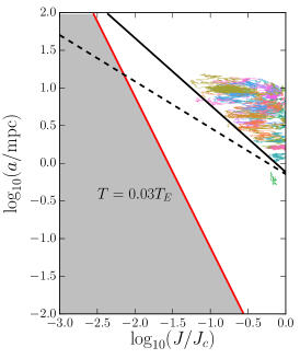
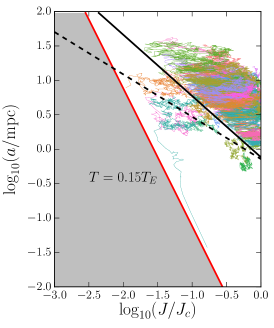
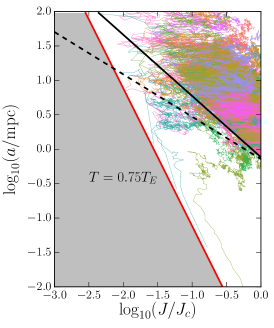
Figure 14.— MC snapshots of the trajectories of individual stars at different times, corresponding to increasing fractions of the energy relaxation timescales $T_{E}$ at $a_{\max}$. On short timescales, $t\ll T_{E}$, stars do not cross the AI line (solid line), while on longer timescales, $t\to T_{E}$, NR progressively drives stellar diffusion across the AI line to the entire available phase-space. The MC simulation assume a MBH of $10^{6}M_{\odot}$ and a cusp of 50 stars of $50M_{\odot}$ each with initial conditions drawn from an isotropic cusp with $\alpha=7/4$ and $a_{\max}=10\,\mathrm{mpc}$. We also plot for comparison the Schwarzschild barrier for this cusp model (dashed line), as suggested by MAMW11.

4.2. Comparison with $N$-body simulations

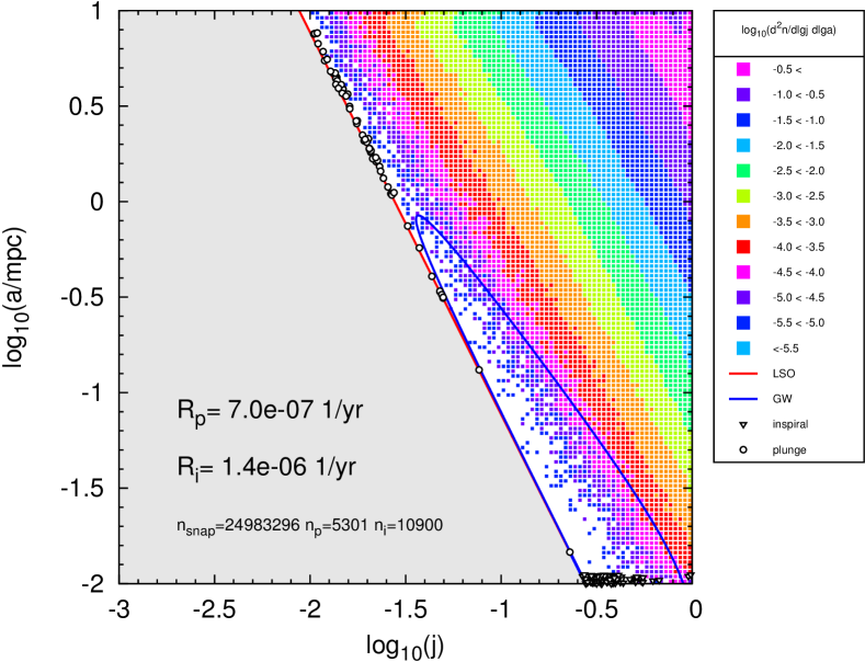
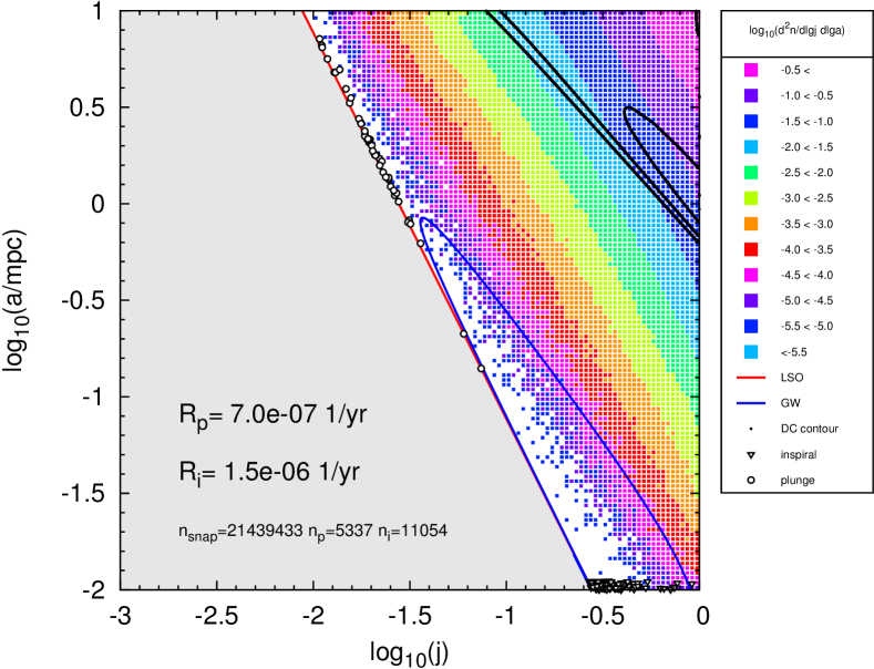
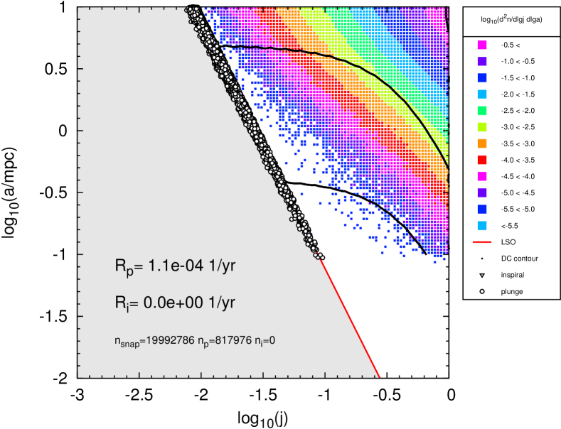
Figure 15.— The 2D loss-cone phase-space density in a MAMW11-like cusp model with mass-precession coherence time and Gaussian noise, calculated by high phase-space resolution MC simulations. Top: Only NR. Middle: Full model with all the dynamical processes. Bottom: Same as full model, with GR precession switched off. The black contours denote the loci where RR dominates NR, $D_{2}^{RR}/D_{2}^{NR}=1,10,100$. To avoid clutter, only 1% of the plunge and inspiral terminal track points (circles and triangles) are displayed.

Matching results of MC simulations to results from direct $N$-body simulations is not straightforward. The MC procedure enforces boundary conditions at $a_{\max}$ and assumes an approximate steady-state background, whereas the $N$-body simulations of MAMW11 and BAS14 provide $a_{\max}$ only as initial conditions (the cluster subsequently expands), and allow the stellar number to fall with time as stars are lost into the MBH. In addition, the MAMW11 and BAS14 models all have an initial $n_{\star}(r)\propto r^{-2}$ cusp, which is away from the BW76 steady-state configuration of a single mass population, $n_{\star}(r)\propto r^{-7/4}$. Thus, these $N$-body simulations always remain out of steady-state due to relaxation, expansion and stellar loss. The loss-rates of the MC (when its parameters are matched to initial state of the $N$-body simulations) should therefore be compared to the initial loss-rates of the $N$-body simulations. To further reduce this incompatibility, we modified our MC procedure to reproduce the initial conditions of the $N$-body simulations by introducing the test stars into the interior of the cusp according to an $n_{\star}\propto r^{-2}$ probability density.

Figure 15 shows the phase-space density derived from MC simulations for the MAMW11 cusp model (see details below), which is used here for comparison with $N$-body results. Results are shown for the case of Newtonian dynamics without RR, and for the case where all dynamical effects are switched on (Newtonian dynamics, GR, NR and RR). Also shown are the endpoints in phase-space of a representative fraction of the plunge and inspiral events. Figure 15 and Table 2 demonstrate that GR precession plays a critical role in making EMRIs possible; in its absence, RR remains unquenched at all low values of $j\geq j_{lc}$ and therefore stars are rapidly driven to plunging orbits before they can reach the EMRI line and inspiral by the emission of GW. However, when GR precession is included, the region where RR dominates over NR is restricted to regions that are far from the loss-lines (black contours, Figure 15 top right). This creates a bottleneck in the flow from $a_{\max}$ and $j\sim{\cal O}(1)$ to the loss-lines, where the orbital evolution is driven by slow NR, and therefore the effect of RR on the loss-rates in steady-state is not large. This near-independence of the steady-state loss-rates from RR is analyzed in Section 3. The MC results also show that mass precession cannot play a similar role, since it becomes efficient only for $j\to 1$ and $a\to r_{h}$ orbits.

Computational costs limited the MAMW11 simulations to a non-realistic cusp of only $N_{\star}=50$ heavy objects of mass $M_{\star}=50\,M_{\odot}$ each around a MBH of mass $M_{\bullet}=10^{6}\,M_{\odot}$, extending between $a_{\min}=10^{-3}$ mpc to $a_{\max}=10$ mpc. The stars were initially set on stable orbits, isotropic in orientation and eccentricity. GR was introduced to the equations of motion perturbatively, up to post-Newtonian (PN) order PN2.5. Orders PN1 and PN2 contribute only to the in-plane (Schwarzschild) periapse precession, while order PN2.5 contributes only to dissipative GW emission. By selectively switching on or off the various PN terms, the $N$-body simulations tested the cases of Newtonian gravity (all PN terms switched off), no GR precession (only the PN2.5 term switched on), or full perturbative GR (all PN terms switched on). Table 2 compares the loss-rates for the corresponding MC and $N$-body simulations, as well as for an artificial model that can only be realized by the MC method, a Newtonian case where RR is switched off. The MAMW11 loss-rates were reported as function of time, so it is possible to extrapolate to $t\to 0$ and obtain lower or upper limits on the rates. The BAS14 rates where reported only in the average.

Table 2 shows that the MC loss-rates for the full GR models are quite similar, irrespective of the RR noise model, and that they are also similar to the rates predicted in the artificial case where RR is switched off. The MC loss-rates are somewhat higher than those derived from the $N$-body simulations. The MC model with smooth (Gaussian) noise provides a better fit to the $N$-body results, while the coherence models are virtually indistinguishable, with only a marginal preference for mass precession.

Overall the MC loss-rates are in agreement with the $N$-body simulations; the systematic trends can be explained by the differences between the computational techniques and the physical assumptions. Compared to the MAMW11 $N$-body simulations, the MC plunge rate is 3.4 higher and the inspiral rate is $1.7$ higher; compared to the BAS14 $N$-body simulations, the MC plunge rate is $1.5\pm 0.3$ higher and the inspiral rate is $1.8_{-0.2}^{+0.2}$ higher. Since the incompatibility of the MC and $N$-body treatment of the boundary condition at $a_{\max}$ results in a lower stellar density in the $N$-body simulations, the fact that the $N$-body loss-rates are systematically lower is to be expected. The same systematic trend is also seen in models where GR is switched off (i.e., no GR precession, no GW). When only GW is switched on but GR precession is switched off (i.e., no GR quenching), the MC inspiral rate is zero in agreement with MAMW11. An additional difference between these studies is the plunge criterion. MAMW11 used $r<8r_{g}$, BAS14 $r<6r_{g}$ and here the criterion was based directly on the angular momentum, $J<J_{lc}$ (where $J$ was evaluated in the Keplerian limit). As noted by Gair et al. (2006), plunging orbits (i.e., parabolic orbits with $J=J_{lc}=4GM/c$) correspond to Keplerian orbits with periapse $r_{lc}=8GM/c^{2}$, or to relativistic orbits with periapse $r_{lc}=4GM/c^{2}$. This can explain some of the systematic differences in the rates, since if $r_{lc}$ over-estimates the true value, stars that should inspiral plunge prematurely, thereby biasing the rates to too-high plunge rates and too-low inspiral rate. Conversely, if $r_{lc}$ under-estimates the true value, a too-high inspiral rate will follow. We believe that this explains the discrepant non-zero inspiral rate that BAS14 find for the case where GR precession is switched off (i.e., Keplerian dynamics where $r_{lc}\to 8r_{g}$ is the correct limit). Our approximate angular momentum plunge criterion for parabolic orbit applies generally in both the Keplerian and relativistic regimes (Gair et al., 2006), unlike the periapse criteria used by the $N$-body simulations. This may explain why the MC inspiral rates are somewhat higher than the $N$-body results, which assume a too-high value of $r_{lc}$ for the relativistic regime.

Table 2The plunge and inspiral rates in MAMW11-like cusp models

Method1	Processes2	$T_{c}$ 3	Noise4	Plunge5	Inspiral5
MC	All	SQ	E	$0.96$	$1.8$
MC	All	SQ	G	$0.71$	$1.5$
MC	All	M	E	$0.92$	$1.8$
MC	All	M	G	$0.71$	$1.4$
MC	No RR	—	—	$0.68$	$1.5$
MC	No GR	M	G	$110$	—
MC	No GR prec.	M	G	$110$	$0$
MC	No mass prec.	M	G	$0.71$	$1.4$
NB1	With GR ($t\to 0$)			$\sim 0.2$	$\sim 0.9$
NB1	No GR ($t\to 0$)			$>20$	—
NB1	No GR prec. ($t\to 0$)			$>20$	$<1$
NB2	With GR			$0.5\pm 0.1$	$0.8\pm 0.1$
NB2	No GR			$28\pm 2$	—
NB2	No Gr prec.			$26\pm 2$	$4.3\pm 0.6$
1 Method: MC = Monte Carlo, NB = $N$-body (1: MAMW11, 2: BAS14).
2 Processes: All includes NR, RR, GW (Gair et al., 2006), mass prec., GR prec.
3 Coherence time: M = Mass prec., SQ = Self-quenching.
4 Noise model: G = Gaussian noise, E = Exponential noise.
5 Event rates in units of $10^{-6}\,\mathrm{yr}^{-1}$.

5. Loss rates

5.1. The Galactic Center test case

The MBH in the center of the Milky Way and the stars and compact objects around it are a system of particular relevance, both because it is uniquely accessible to observations, and can therefore place constraints on dynamical models and theories Alexander (2005), and because planned space-borne GW detectors with ${\cal O}(10^{6}\,\mathrm{km})$ baseline will be optimally sensitive to GWs emitted by a mass orbiting a $10^{6}-10^{7}\,M_{\odot}$ MBH near the last stable orbit (Amaro-Seoane et al., 2007). Therefore, although it remains an open question whether the Galactic center (GC) is surrounded by a high density relaxed cusp of stellar remnants (see review by Alexander, 2011), and although the rate of GW events from the GC itself is expected to be small (but see Freitag, 2003), the Galactic MBH SgrA^⋆ represents the archetypal cosmic GW target.

We adopt here a simplified model of the GC consisting of an MBH mass of $M_{\bullet}=4\times 10^{6}\,M_{\odot}$, surrounded by a steady-state $\alpha=7/4$ cusp of equal mass stars of either $M_{\star}=1\,M_{\odot}$ or $10\,M_{\odot}$, extending between $a_{\mathrm{\min}}=2\times 10^{-4}\,\mathrm{pc}$ ($a_{\mathrm{in}}=0.1a_{\min}$, see Appendix B) to $a_{\mathrm{out}}=a_{\max}=r_{h}=2\,\mathrm{pc}$ with a total stellar mass of $M_{\star}N_{\star}(<r_{h})=2M_{\bullet}$ inside the radius of influence. Test stars are injected into the nucleus with initial sma $a_{0}=a_{\mathrm{out}}$, and with isotropic $j_{0}$.

Figure 16 shows the steady-state configuration and loss-rates for a GC model with $M_{\star}=10\,M_{\odot}$ and a smooth background noise whose coherence is set by mass precession. As expected from the fact that the RR-dominated region in phase-space is well separated from the loss-lines, the steady-state phase-space density is very close to the simple NR-only solution.

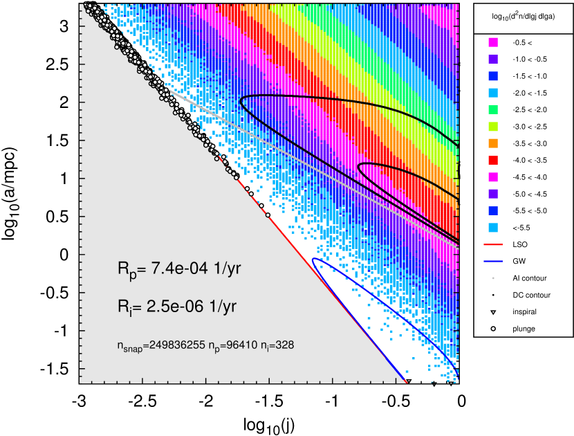
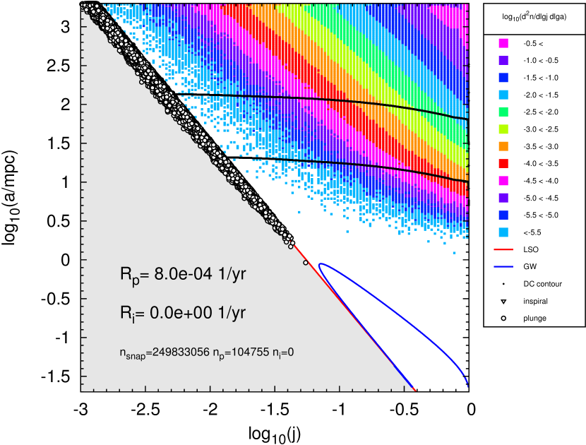
Figure 16.— The 2D loss-cone phase-space density in a Milky Way-like cusp model with mass-precession coherence time and Gaussian noise, calculated by high phase-space resolution MC simulations. Stars / stellar mass BHs of $10\,M_{\odot}$ are assumed. Top: GR precession included. Mass precession limits the efficiency of RR beyond $\sim 100\,\mathrm{mpc}$, while GR precession limits RR below the AI locus (gray line). RR is faster than NR only well away from the loss-cone, inside the black contours (equally fast at the outer contour, 10 times faster at the inner contour). Bottom: When GR precession is artificially switched off, RR remain effective all the way down to the loss-cone and is faster than NR below $a\sim 100\,\mathrm{mpc}$. As a result, stars are driven to plunge trajectories well before they can lose enough energy by NR to reach the GW loss-line. A central, strongly depleted cavity is formed, and the EMRI rate is completely suppressed.

Table 16 explores the implications of varying some of the assumed processes for the loss-rates: the mass of the cusp stars ($1\,M_{\odot}$ or $10\,M_{\odot}$), the nature of relaxation (NR only, or NR and RR) the noise model (White, exponential, Gaussian), the coherence mechanism (mass precession, self-quenching), or the GW dissipation approximation.

Table 3The plunge and inspiral rates in Milky Way-like cusp models

$M_{\star}$ 1	Processes2	$T_{c}$ 3	Noise4	Plunge5	Inspiral5
$1$	No RR	—	—	$730$	$3.1$
$1$	GW1	SQ	W	$16000$	$0.0$
$1$	GW1	SQ	E	$860$	$3.3$
$1$	GW1	SQ	G	$880$	$2.3$
$1$	GW1	M	W	$930$	$0.0$
$1$	GW1	M	E	$840$	$3.2$
$1$	GW1	M	G	$840$	$3.2$
$10$	No RR	—	—	$610$	$2.8$
$10$	GW1	SQ	W	$6060$	$0.0$
$10$	GW1	SQ	E	$760$	$1.9$
$10$	GW1	SQ	G	$690$	$2.4$
$10$	GW1	M	W	$800$	$0.0$
$10$	GW1	M	E	$730$	$2.0$
$10$	GW1	M	G	$730$	$2.5$
$10$	GW2	M	G	$730$	$1.2$
$10$	GW3	M	G	$740$	$1.1$
1 Stellar mass in $M_{\odot}$.
2 GW approximations: GW1 Gair et al. (2006), GW2 Peters (1964),
GW3 Hopman & Alexander (2006a)
3 Coherence time: M = Mass prec., SQ = Self-quenching.
4 Noise model: W = White, E = Exponential, G = Gaussian.
5 Event rates in units of $10^{-6}\,\mathrm{yr}^{-1}$.

The uncorrelated (white) noise model for the resonant torques, which is equivalent to the assumption that $\nu_{GR}\to 0$, results in very high plunge rates as strong RR rapidly drains the cusp, and as a result the EMRI rate drops to zero. In contrast, for all other RR models, irrespective of the assumptions about the nature of the noise or the coherence mechanism, GR precession suppresses RR to the extent that rates are very similar to those derived for the non-physical “NR-only” model: a plunge rate of $\Gamma_{p}\sim(6-9)\times 10^{-4}\,\mathrm{yr^{-1}}$, and an inspiral rate of $\Gamma_{i}\sim(1-3)\times 10^{-6}\,\mathrm{yr}$. We find that the more sophisticated GW dissipation estimate of Gair et al. (2006) results in inspiral rates that are a factor $\sim 2$ higher than the estimates by Peters (1964) or Hopman & Alexander (2006a). We conclude that to within a factor of $\sim 2$, our rate estimates for relaxed steady-state cusps are robust to variations of the physical assumptions.

5.2. Scaling with the MBH mass

The MC simulations can be used to validate a simple analytic model for estimating the loss-rates and their dependence on the parameters of the galactic nucleus, which is based on identifying critical values of the sma, $a_{c}$, below which the probability of a star to cross the loss-line is ${\cal O}(1)$ (Lightman & Shapiro, 1977; Hopman & Alexander, 2005). The loss-rate is then $\Gamma\propto N(<a_{c})/T_{NR}(a_{c})$, where the proportionality factor includes the suppression of the density near the loss-line. For plunge events $a_{c}\sim{\cal O}(r_{h})$ (Lightman & Shapiro, 1977), while for GW inspiral $a_{c}\sim a_{GW}\ll r_{h}$, the maximum of the GW line (Section 3). Figure 1 shows that the region of phase-space where RR dominates the dynamics is well separated from the loss-lines, is well below $r_{h}$ and well above $a_{GW}$. The timescale relevant for estimating is therefore that of NR and not RR.

In order to estimate the integrated cosmic rates of EMRIs or tidal disruption flares, it is necessary to scale the loss-rates by the parameters of the host galaxy, in particular the MBH mass. Here we adopt a simplified one-parameter sequence of galactic nuclei, where the free parameter is $M_{\bullet}$, which together with several additional fixed parameters define the sequence. The $M_{\bullet}$-scaling is based on the empirical $M_{\bullet}/\sigma$ relation $M_{\bullet}=M_{0}(\sigma/\sigma_{0})^{\beta}$ where $\sigma$ is the stellar velocity dispersion outside the MBH radius of influence $r_{h}=\eta_{h}GM_{\bullet}/\sigma^{2}$, which encloses a stellar mass of order the mass of the MBH $N_{\star}(r_{h})=\mu_{h}Q$. The power law parameter $\beta\sim 4-5$ and the normalization $M_{0}/\sigma_{0}^{\beta}$ are determined empirically (Ferrarese & Merritt, 2000; Gebhardt et al., 2000). It then follows that $r_{h}=\eta_{h}\left(M_{\bullet}/M_{0}\right)^{1-2/\beta}GM_{0}/\sigma_{0}^{2}$ (Alexander, 2011).

Using this parameterization, and the approximation that the steady-state distribution is given by a BW76 cusp, the total plunge and inspiral rates can be estimated from Eqs. (29) and (32),

$$R_{p}^{\mathrm{tot}} \approx \frac{10\mu_{h}^{2}}{\eta_{h}^{3/2}}\frac{\sigma_{0}^{3}}{2\pi GM_{0}}\left(\frac{M_{\bullet}}{M_{0}}\right)^{3/\beta-1}$$

$$\times\frac{\log Q}{\log\left[\sqrt{\eta_{h}}\left(M_{0}/M_{\bullet}\right)^{1/\beta}\left(c/4\sigma_{0}\right)\right]}\,,$$

and

$$R_{i}^{\mathrm{tot}} \approx A_{GW}\frac{10\mu_{h}^{6/5}}{\eta_{h}^{3/2}}\frac{\sigma_{0}^{3}}{2\pi GM_{0}}\left(Q_{0}\right)^{3/\beta-1}$$

$$\times\frac{\left(\log Q\right)^{1/5}}{\log\left[\sqrt{\eta_{h}A_{GW}}\left(\mu_{h}\log Q\right){}^{-2/5}Q_{0}^{-1/\beta}c/\left(4\sigma_{0}\right)\right]}\,,$$

where $Q_{0}=M_{\bullet}/M_{0}$, $a_{GW}=A_{GW}\left(\mu_{h}\log Q\right){}^{-4/5}$ and $A_{GW}$ is a numerical factor which depend on the GW dissipation approximation (Appendix A).

In our MC simulations, we adopted for simplicity $\beta=4$, $\mu_{h}=2$, $\eta_{h}=1$, $M_{0}=5.4\times 10^{6}\,M_{\odot}$ and $\sigma_{0}=100\,\mathrm{km\,s^{-1}}$. Thus

$$r_{h}=2\left(M_{\bullet,MW}\right)^{1/2}\,\mathrm{pc},$$ (45)

where $M_{\bullet,MW}=M_{\bullet}/4\times 10^{6}M_{\odot}$ is the MBH mass scaled to the mass of the Galactic MBH. The rates as function of the MBH mass $M_{\bullet}$ and the mass ratio $Q=M_{\bullet}/M_{\star}$ are then

$$R_{p}^{\mathrm{tot}} = 3\times 10^{-4}M_{\bullet,MW}^{-1/4}$$

$$\times\frac{\log Q}{6.70-0.25\log\left(M_{\bullet,MW}\right)}\,\mathrm{yr^{-1}}\,,$$

and

$$R_{i}^{\mathrm{tot}} \approx 5\times 10^{-6}M_{\bullet,MW}^{-1/4}$$

$$\times\frac{\left(\log Q\right)^{1/5}}{4.65-0.25\log\left(M_{\bullet,MW}\right)-2\log\left(\log Q\right)/5}\,,$$

where we used the value $A_{GW}\approx 0.029$, corresponding to the GW dissipation approximation of Gair et al. (2006) (Appendix A). As shown in Figure 17, these analytic approximations are in agreement with the results of the MC simulations over several orders of magnitude of $M_{\bullet}$.

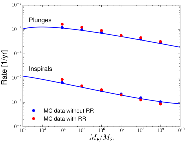
Figure 17.— The total Plunge and inspiral rates as a function of MBH mass. The MC simulations (circles) agree with the analytic approximations for dynamics without RR (solid lines), Eqs. (LABEL:eq:RpMW), (LABEL:eq:RiMW). Simulations with RR show that the contribution of RR is small: the discrepancy between the rates with and without RR does not exceed $\sim 30\%$ over 5 orders of magnitude in $M_{\bullet}$.

6. Discussion and summary

The determination of the steady-state of galactic nuclei is a fundamental open question in stellar dynamics, with many implications and ramifications, and has been the focus of numerous numerical and analytical studies. In particular, current estimates of loss-rates vary over several orders of magnitude due to theoretical and empirical uncertainties. Previous studies either used post-Newtonian $N$-body simulations, which are limited to small-$N$, or did not include the relevant relativistic physics (Section 1). Building on recent progress in the formal description of RR as a correlated diffusion process (the $\boldsymbol{\eta}$-formalism, Bar-Or & Alexander 2014), we obtain here a MC procedure and analytic expressions for the steady-state distribution and loss-rates in galactic nuclei, taking into account two-body relaxation, RR, mass precession and the GR effects of in-plane precession and GW emission. By cross-validating the analytic estimates and the MC results with a high degree of accuracy, and without the introduction of any free fit parameters, we are able to confirm our analysis and interpretation of the dynamics of the loss-cone in the context of our underlying assumptions.

6.1. Discussion of main results

The advantage of modeling RR by the $\boldsymbol{\eta}$-formalism, over previous attempts by other approaches (Rauch & Tremaine, 1996; Hopman & Alexander, 2006a; Gürkan & Hopman, 2007; Madigan et al., 2011; Merritt et al., 2011; Antonini & Merritt, 2013; Hamers et al., 2014; Merritt, 2015a, b), is that it allows to derive the FP equation rigorously from the stochastic leading-order relativistic 3D Hamiltonian. The resulting effective DCs, which are thus derived from first principles, are then guarantied to obey the fundamental fluctuation-dissipation relation and the correct 3D maximal entropy solution (Binney & Tremaine 2008, Section 7.4.3; Appendix E).

These constraints on the functional form of valid DCs are critical, since the correct steady-state is the result of a fragile near-cancellation of two large opposing currents (the diffusion and drift); even small deviations from this relation (e.g., due to approximations, empirical fits, or reduction to lower dimensions), will result in large errors. For example, Hamers et al. (2014) obtained the RR DCs from numerical simulations using an assumed functional form, $D_{jj}\propto\sqrt{1-j^{2}}$, based on the fit of Gürkan & Hopman (2007) and on the ad hoc expression $D_{j}=j^{-1}D_{jj}$, which is inconsistent with the fluctuation-dissipation relation and therefore leads to invalid steady-sate solution. This was then partially remedied by Merritt (2015a) who treated separately the Newtonian ($j\to 1$) and relativistic ($j\to 0$) regimes. In the Newtonian regime, the Hamers et al. (2014) data was re-fitted to DCs that effectively satisfy the fluctuation-dissipation relation, which means that in the absence of a loss-cone, the dynamics asymptote to the maximal entropy limit $n(j)=2j$. However, in the relativistic limit $j\to 1$, where the simulation statistics are poorer due to the smaller phase-space volume, Merritt (2015a) used analytic DCs based on the Hamiltonian model of Merritt et al. (2011), which represented the stochastic background by an ad hoc dipole pseudo-potential and a recipe for switching its direction every coherence time. This recipe corresponded to the $\boldsymbol{\eta}$-formalism’s “Steps” or “Exponential ACF” noise (depending on the exact switching procedure), which both converge to the same form in the $j\to 0$ limit (Bar-Or & Alexander, 2014, Figure 1). As shown by Bar-Or & Alexander (2014, Eq. 42), in that limit $D_{jj}\approx j^{4}/\tilde{T}_{c}$ and $D_{j}\approx(5/2)j^{3}/\tilde{T}_{c}$, where $\tilde{T}_{c}=0.5T_{c}\nu_{GR}^{2}\left(j=1\right)/\nu_{j}^{2}\left(j=0\right)$. This indeed satisfies the fluctuation-dissipation relation, as any Hamiltonian model is guaranteed to do. These DCs are different from the ones derived by Merritt (2015a), $D_{jj}\propto j^{4}/T_{c}$ and $D_{j}=2D_{jj}/j$, who implicitly forced the solution to 2D in-plane motion by setting $\sin i=1$ in the derivation (Merritt, 2015a, Eqs.C.8-C.9). Therefore, these derived DCs satisfy the 2D fluctuation-dissipation relation $2D_{j}=\partial D_{jj}/\partial j$, rather than the correct 3D one, $2jD_{j}=\partial jD_{jj}/\partial j$. These DCs therefore imply the steady-state solution $n(j)=\mathrm{const}$ in the relativistic regime (assuming no loss-cone); this is not the correct solution for 3D orbital motion (the correct one is $n(j)=2j$). We note that the concatenation of two diffusion solutions, a 3D one for the Newtonian regime and a 2D one for the relativistic regime, may create an artificial discontinuity in the dynamical behavior at the interface.

We have shown that the representation of stochastic dynamics near a MBH in terms of the streamlines of the probability flow provides a powerful tool for analyzing the loss fluxes, and leads to the identification of the exact separatrix between plunges and inspirals. We show that the typical sma of this separatrix, $a_{GW}$, yields an excellent analytical estimate for the inspiral rates found in our MC simulations (Figure 17). This remedies the ambiguity in the identification of the critical sma, which was used to estimate rates in previous studies. We also explored the effect of different GW dissipation approximations on $a_{GW}$ and the resulting GW inspiral rate, and found that the rates are robust to within a factor 2. Nevertheless, it is worth noting that the more accurate method of Gair et al. (2006) predicts EMRI rates that are more than twice higher than those of the commonly used approximation of Peters & Mathews (1963).

We have shown that GR precession plays a critical role in the dynamics of the loss-cone by efficiently quenching the RR torques. Conversely, in its absence all stars would rapidly plunge into the MBH, creating a depleted central cavity (cf Figure 16). This implies that GR precession is important even in systems that are effectively Newtonian, where at any given time only a very small fraction of the stars are on relativistic orbits. In particular, $N$-body simulations of stellar dynamics and stellar populations near MBHs should include GR precession even if the questions of interest are in the non-relativistic regime, so that plunges do not compete, or limit the lifetime of the stars. It is worth noting that GR precession has not yet been tested empirically for relativistic parameters larger than $\Upsilon=2GM_{\bullet}/c^{2}r>8\times 10^{-6}$ (the double pulsar system PSR J0737-3039, Lyne et al. 2004), whereas the S-stars in the Galactic center, for example, are already observed to reach $\Upsilon=2GM_{\bullet}/c^{2}r>1\times 10^{-3}$ at periapse (star S14, Gillessen et al. 2009a, see also Alexander 2006). Moreover, near the relativistic loss-cone ($r_{p}=4r_{g}$, Gair et al. 2006), where $\Upsilon\to 1/2$, there is to date no empirical confirmation of GR precession (Will, 2006). The existence, dynamics and loss-rates of stars on such relativistic orbits can therefore probe GR precession in the strong field limit.

We have shown that the influence of RR on steady-state loss-cone dynamics of compact objects is a small ${\cal O}(1)$ effect, since the loss-lines for both direct plunge and GW inspiral lie well outside the region where RR is effective (e.g., Figure 1). RR does introduce a correction to the steady-state distribution and the loss-rates, which is at present small in comparison to the astrophysical uncertainties, such as stellar density and mass function, the $M_{\bullet}/\sigma$ relation, and deviations from spherical symmetry. Eqs. (LABEL:eq:Rp–LABEL:eq:RiMW) provide useful analytic estimates for the plunge and inspiral rates per galaxy, based on the NR-only approximation. The RR correction to the rates can be obtained by numerical integration of Eq. (42). Using a suite of MC simulations, we have verified in the context of our assumptions that the rate estimates are robust under different assumptions about the properties of the stellar background noise (smoothness, coherence time). This is in large measure a reflection of the limited role of RR in the presence of continuous noise (Bar-Or & Alexander, 2014, Figure 1), which restricts the domain where RR is effective, so that slow NR remains the bottleneck and sets the rates.

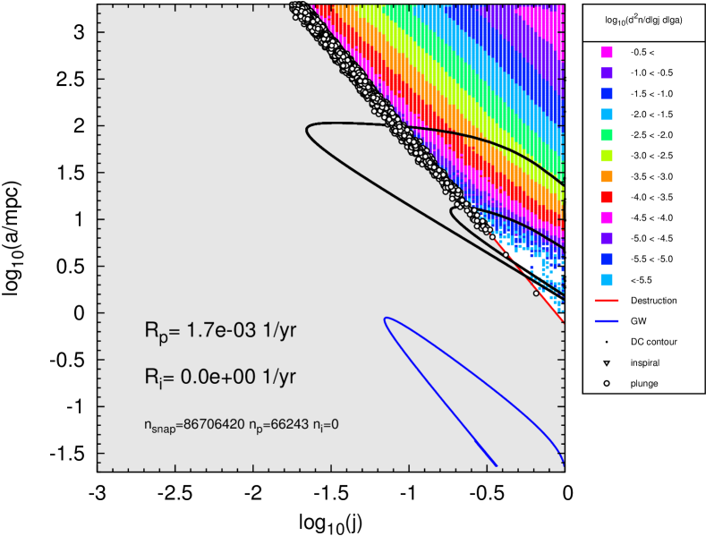
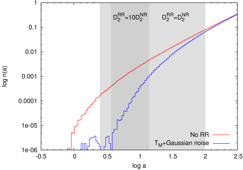
Figure 18.— The suppression of the phase-space density of icy planetesimals around a MBH due to RR-driven interactions with a circumnuclear accretion disk. Top: The phase-space density and the disk interaction loss-line. The black contours delineate the region where RR dominates ($D_{2}^{RR}/D_{2}^{NR}=1,10$). Bottom: The resulting steady-state $a$-distribution of the planetesimals for the NR-only case, and for the full dynamical model (top panel). The shaded regions denote the $a$-intervals where the loss-line crosses regions where RR dominates.

RR can substantially affect processes whose loss-lines intersect the phase-space region where RR dominates ($D_{2}^{RR}\gg D_{1}^{RR}$ ). The loss lines for tidal disruption of extended objects by the MBH, such as red giants or binaries, do lie closer to the RR line. However, it can be readily shown that neither class of objects is long-lived enough for RR-driven tidal destruction to play a dominant role in Milky Way-like galactic centers. Red giants are relatively short-lived, and the more extended and tidally-susceptible they are, the shorter their lifespan. Soft stellar binaries are destroyed by 3-body ionization before they are affected by RR-driven tidal separation (Alexander & Pfuhl, 2013).

One class of processes where RR may have more than an ${\cal O}(1)$ effect is the hydrodynamical destruction (or removal) of objects by interaction with a large circumnuclear accretion disk. To demonstrate this point, we consider here as an idealized simple example the case of a massive accretion disk of radius $R_{d}=2000r_{g}$ (Goodman, 2003) and a population of long-lived icy planetesimals around it, which are destroyed by several consecutive disk crossings (it is assumed that the number of crossings for destruction is $N_{\mathrm{cross}}P\ll T_{NR}$). In that case, the critical angular momentum for destruction is $j_{d}=\sqrt{2GM_{\bullet}R_{d}}=15.8j_{lc}$, which is large enough to intersect the RR-dominated zone (Figure 18 top). As a result, the differential sma distribution of the planetesimals is depleted below $a\lesssim 100\,\mathrm{mpc}$ and strongly so below $a\lesssim 10\,\mathrm{mpc}$ (Figure 18 bottom).

Although RR is typically inefficient in driving stars all the way to the loss-cone, it can randomize orbits in the phase-space regions where it dominates, even when the NR timescale is longer than the system’s age or the lifespan of the stars. This may be a key element in solving the “paradox of youth” (Ghez et al., 2003) in the Galactic Center, where young B stars are observed on tight orbits around SgrA^⋆ (the so-called “S-star” cluster). The leading formation or migration scenarios for the S-stars predict non-isotropic initial eccentricities (see reviews by Alexander, 2005, 2011). However, most of the S-stars are in the RR-dominated phase-space region (Figure 1), and so substantial evolution and isotropization of the initial eccentricities is possible. However, many of the S-stars are short-lived, and some are close in phase-space to the AI-suppressed region. A detailed analysis using the $\boldsymbol{\eta}$-formalism, which can treat this intermediate dynamical regime rigorously, has yet to be carried out.

6.2. Limitations and caveats

The applicability and validity of our results are limited by several simplifying assumptions. We assume a non-spinning MBH surrounded by an isotropic (on average) non-rotating single Keplerian power-law cusp of single-mass stars. We assume the dynamics are dominated by single star interactions, that is, we neglect the possible effects of binaries, or the contribution of non-stellar massive perturbers, such as gas clouds, cluster or intermediate mass BHs (Perets et al., 2007).

In our MC simulations we used NR and RR DCs, which are based on a fixed isotropic, single power-law BW76 model. These DCs are therefore not self-consistent with the steady-state solution. However, we showed that the BW76 cusp is a good approximation (within a factor of two) for the steady-state solution in the relevant region (down to $a_{BW}<a_{GW}$ for $M_{\bullet}\lesssim 10^{9}M_{\bullet}$; see Section 3.4). In addition, it can be shown that for the RR DCs the isotropic fluctuation-dissipation relation holds even for the non-isotropic case as long as the total angular momentum of the system is zero (Bar-Or & Alexander, 2014). Since the fluctuation-dissipation relation results from the symmetries of the Hamiltonian, it is reasonable to assume that the same will hold also for the NR DCs. This means that small non-isotropies will only result in small magnitude changes of the flux and have little effect on the steady-state distribution.

Finally, the RR DCs are based on simplified (single timescale) background noise models that can be treated analytically, and simple coherence models that are functions of the sma only. However, we were able to show using MC simulations that the results are largely independent of the exact noise model as long as it is continuous (i.e., not white noise).

Appendix A The analytic gravitational wave line

The phase-space of the relativistic loss-cone is divided by a separatrix into an outer region where streamlines end as plunges, and an inner region where streamlines end as inspirals (Figure 4). Since the probability current along an infinitesimal bundle of streamlines is conserved (Section 3.5), it can be evaluated at any convenient point along the flow, in particular at $J\gg J_{lc}$, where GWs are negligible, and the streamlines are identical to those in the absence of GWs. Therefore, the inspiral rate is estimated by locating the no-GW plunge streamline that corresponds to the separatrix, and identifying the sma of its terminal point ($a_{p},j_{lc}$) as the critical (maximal) sma for inspiral, $a_{GW}$. The inspiral rate is then simply the integrated plunge rate in the absence of GW, up to $a_{GW}$, i.e., $R_{i}^{\mathrm{tot}}=R_{p}^{no\,GW}\left(a_{GW}\right)$.

The separatrix streamline, $\mathrm{d}E/\mathrm{d}J=S_{E}/S_{J}$, can be evaluated by noting that the flow in the $E$-direction is mostly due to GW dissipation,

$$S_{E}=n\left(E,J\right)E/t_{GW}\,,$$ (A1)

where $t_{GW}\equiv a/\left|\dot{a}_{GW}\right|$ is the GW orbital decay timescale. In the presence of GW, the innermost plunge streamline initially approaches $j_{lc}$ from $j\sim 1$ at nearly constant $a$, and then turns over to lower $a$ and runs nearly parallel to the loss-line $j_{lc}(a)=4\sqrt{r_{g}/a}$ until it terminates when $j\to j_{lc}$ at some small enough terminal sma, $a_{insp}$, where the orbital motion is effectively circular (i.e., inspiral, cf Figure 4). For example, for parabolic orbits, the minimal possible value for $a_{insp}$ is obtained where $j_{lc}=1$, i.e., for $a_{insp}=16r_{g}$. As we demonstrate below (Eq. (A9)), the separatrix solution is a function of $a_{insp}$ only via $a_{insp}/a_{\max}\ll 1$, and is therefore independent of the exact choice of $a_{insp}$.

The flow in the $J$-direction is approximately constant in $J$ with a typical timescale $T_{J}$ (Eq. (16)),

$$S_{J}\approx-\frac{n\left(E\right)}{T_{J}\log\left(J/J_{lc}\right)}\,.$$ (A2)

Since RR is negligible near $j=j_{lc}$, $T_{J}$ can be approximated as $T_{J}\left(a\right)\approx\theta_{\gamma}Q^{2}P\left(a\right)/\left(N\left(a\right)\log Q\right)$ (see Eq. (19)), where $\theta_{\gamma}$ is a numeric pre-factor that depends on the cusp density profile ($\theta_{\gamma}\approx 1/8$ for a $\gamma=7/4$ (BW76) cusp).

It then follows that separatrix is the solution of the differential equation

$$\frac{dE}{dJ}=\frac{S_{E}}{S_{J}}\approx-2\frac{J}{J_{c}^{2}}T_{J}\frac{E}{t_{GW}}\log\left(\frac{J}{J_{lc}}\right)\,,$$ (A3)

with the boundary condition $J(E_{insp})=J_{lc}$ (where $E_{insp}=GM_{\bullet}/2a_{insp})$.

An exact expression for the GW dissipation can be obtained only numerically. Some useful analytical approximations are available (see Gair et al. (2006) for a comparison between the different techniques). The simplest expression was obtained by Peters & Mathews (1963), who assumed a point-mass objects moving on a Keplerian orbit. In this approximation the GW timescale is

$$t_{GW}\equiv\frac{a}{\left|\dot{a}_{GW}\right|}=\frac{1}{2\pi}\frac{5}{64}\frac{Q}{f(e)}\frac{r_{g}}{a}\left(\frac{2r_{p}}{r_{g}}\right)^{7/2}P\left(a\right)\,,\,\,\,f(e)=\left(\frac{1+e}{2}\right)^{-7/2}\left(1+\frac{73}{24}e^{2}+\frac{37}{96}e^{4}\right)\,,$$ (A4)

In the limit $J\to J_{c}$, the periapse $r_{p}$ is related to the angular momentum by $r_{p}/r_{g}=8J^{2}/J_{lc}^{2}$ and the streamline equation (Eq. (A3)) can be written in terms of $x=a/a_{\max}$ and $s=J/J_{lc}$,

$$\frac{dx}{ds}=A_{D}x^{\gamma-2}s^{-6}\log\left(s\right)\,,$$ (A5)

where the competition between the GW dissipation and NR diffusion is expressed by the parameter

$$A_{D}=\frac{\pi}{20}f(1)\frac{\theta_{\gamma}Q}{N_{h}\log Q}\sim{\cal O}(10^{-3})\,.$$ (A6)

The boundary condition at the terminal sma is

$$x_{1}\equiv x\left(s=1\right)=a_{insp}/a_{\max}\ll 1,$$ (A7)

and the plunging branch of the solution is give by

$$x\left(s\right) = \left[x_{1}^{3-\gamma}+\frac{A_{D}\left(3-\gamma\right)\left(s^{5}-5\log s-1\right)}{25s^{5}}\right]^{1/\left(3-\gamma\right)}\,.$$ (A8)

In the phase-space region where GW is negligible, the streamline defined by Eq. (A3) is approximately constant in $E$. Therefore, $a_{GW}$ can be identified by the sma at $s\gg 1$ ($j\to 1$), that is

$$a_{GW}\approx a_{\max}\lim_{s\to\infty}x=\left(x_{1}^{3-\gamma}+\frac{\left(3-\gamma\right)}{25}A_{D}\right)^{1/\left(3-\gamma\right)}a_{\max}\,.$$ (A9)

For a steady-state cusp (i.e., BW76, $\gamma=7/4$), $x_{1}^{3-\gamma}\ll(3-\gamma)A_{D}/25$, and therefore

$$a_{GW}\approx A_{GW}\left(\frac{N_{h}\log Q}{Q}\right)^{-4/5}a_{\max}$$ (A10)

where the value of $A_{GW}$ depends on the specific GW dissipation approximation that is assumed. For the Keplerian approximation $A_{GW}^{K}=(\pi f(1)/3200)^{4/5}\approx 0.013$.

As shown by Gair et al. (2006), the Peters & Mathews (1963) estimate can be improved by using a “semi-relativistic” approximation, that is using the fully relativistic orbit in place of the Keplerian one in Peters & Mathews (1963) equations. In the limit $e\to 1$, this approach, used by Hopman & Alexander (2005), amounts to replacing the Keplerian $r_{p}/r_{g}$ in Eq. (A4) with the relativistic one (Gair et al., 2006)

$$r_{p}/r_{g}=4s\left(s+\sqrt{s^{2}-1}\right)\,.$$ (A11)

Thus the GW separatrix (Eq. (A5)) is replaced by its relativistic version,

$$\frac{dx}{ds}=2^{7/2}A_{c}x^{\gamma-2}\left(1+\sqrt{1-1/s^{2}}\right)^{-7/2}s^{-6}\log\left(s\right)\,,$$ (A12)

where $a_{GW}$ can be solved numerically. As shown in Figure 19, $a_{GW}$ can be approximated for $\gamma=7/4$ by Eq. (A10) with $A_{GW}^{R}=0.022$ and for the more accurate treatment of Gair et al. (2006), $A_{GW}=0.029$, which is adopted in this study.

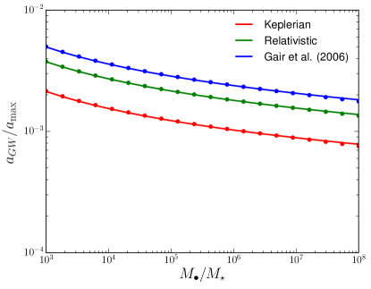
Figure 19.— The semi-major axis $a_{GW}$ of the outermost inspiraling streamline for a BW76 cusp ($\gamma=7/4$) for different MBH to star mass ratios and for different approximations of the GW dissipation. The approximate expression (Eq. (A10)) for $a_{GW}$ (lines) is fitted to values of $a_{GW}$ found by numerically integrating the streamline equation (Eq. (A3)) (circles).

Appendix B Monte-Carlo simulations of loss-cone dynamics

We summarize here the assumptions underlying our Monte-Carlo (MC) simulations, the details of the implementation and the derivation of the steady-state configuration and loss-rates.

B.1. Assumptions and procedure

The MC simulations in $(a,j)$ assume a fixed background model, whose properties define the NR diffusion coefficients, an RR coherence timescale model and a background noise model. The stellar background is approximated as a power-law cusp with enclosed number of stars $N(a)=N_{\max}(a/a_{\max})^{3-\alpha}$, extending between $a_{\min}$ and $a_{\max}$. The accessible phase-space for the test stars extends between a reflecting boundary at $a_{\mathrm{out}}=a_{\max}$ (evaporation), and an absorbing boundary at $a_{\mathrm{in}}<a_{\min}$ (destruction). The reflective boundary at $a_{\mathrm{out}}$ ensures that the long-term distribution of test stars converges to an isotropic distribution in $j$, $n(j)\to 2j$, which is the assumed distribution of stars far from the MBH (note that this is not guaranteed for an absorbing outer boundary, even when the test stars are introduced into the simulation isotropically). The extension of phase-space to small $a_{\mathrm{in}}$ allows inspiral trajectories to be tracked down to a tight enough sma where their ultimate fate as EMRIs is certain (cf Figure 15) phase-space extends in $j$ between a reflecting boundary at $j=1$ and an absorbing boundary at the last stable orbit (LSO), $j_{LSO}$, defined by the locus $J_{LSO}(a)=\sqrt{a/r_{g}}j_{LSO}=4r_{g}c$ (the LSO for a zero energy orbit in the Newtonian approximation; in the limit $e\to 1$ it corresponds to a critical periapse $r_{LSO}=a(1-e)=8r_{g}$).

An MC run starts by injecting a test star in some initial phase-space position $(a_{0},j_{0})$. This is typically chosen randomly, either just below $a_{\max}$, with $j$ distributed isotropically above $j_{LSO}$, to simulate a star diffusing from an isotropic galaxy into the MBH’s radius of influence, or isotropically in the cusp’s bulk, according to the power-law cusp distribution, to simulate the initial conditions of an $N$-body simulation (see below), or the distribution of tracer stars (e.g., red giants), which mirror the distribution of cusp stars. The star is then evolved in small time increments $\mathrm{d}t$, taking into account the stochastic changes in energy and angular momentum due to NR, the deterministic changes due to GW dissipation, and the random changes in angular momentum due to RR. The star is tracked in phase-space, and its position is recorded by snapshots taken at fixed intervals $\Delta t\gg\mathrm{d}t$. Ultimately, after surviving for time $t_{s}$, the star leaves the system at some terminal phase-space position $(a_{1},j_{1})$ as a result of one of four possible outcomes. $(1)$ Evaporation. The star’s sma crosses $a_{\mathrm{out}}$ to a larger sma. This happens for the majority of test stars. (2) Inspiral. The star’s orbit decays until it crosses $a_{insp}=\epsilon a_{\min}$ mpc ($\epsilon\ll 1$). (3) Plunge. The star crosses the LSO directly, at some $a_{p}>a_{insp}$. (4) Finite lifespan exceeded. This is relevant for stars, which are limited by stellar evolution or for binaries, which are also limited by dynamical evaporation (Section 6.1), but not for compact remnants. Note that the branching ratio between plunges and inspirals is independent of the exact value of the sma chosen to distinguish between the two outcomes (parameterized by $\epsilon$), since their respective terminal phase-space positions are clearly separated ($\min a_{\mathrm{plunge}}\gg a_{\mathrm{inspiral}}$, cf Figure 15; $\epsilon=0.1$ was typically used here).

Once a star exits the system, a new star is injected (reflection at $a_{\mathrm{out}}$ is equivalent to injection of a new star at $(a_{\mathrm{out}},j_{1})$). This is repeated over some long accumulated time $T_{\mathrm{sim}}\gg t_{s}$ (typically $T_{\mathrm{sim}}\sim 100T_{E}$, Section 3.4). All test stars simulated over $T_{\mathrm{sim}}$, apart for the last one, which is omitted from the analysis, reach a definite outcome. For each test star we record its trajectory in phase-space (in coarse $\Delta t$ resolution); the total time it spent evolving in phase-space, $t_{s}$; the nature of the final outcome (evaporation, inspiral, plunge or end of lifetime); and its initial and terminal phase-space positions. The procedure is repeated as needed (typically $10^{3}-10^{4}\times T_{\mathrm{sim}}$), until enough test star statistics are collected. The snapshots of the phase-space positions, the survival times and the final outcomes are then used to estimate the steady-state configuration and loss-rates, as detailed below.

B.2. Representation of physical processes

The form of the RR DCs depend on the background noise model and the precession of the test star (Bar-Or & Alexander, 2014). We assume three optional noise models: white noise (equivalent to no precession), $C^{0}$ noise with exponential ACF (an Ornstein-Uhlenbeck process), and smooth $C^{\infty}$ noise with a Gaussian ACF. Prograde GR in-plane precession is modeled by the 1PN approximation $\nu_{GR}=3\nu_{r}(a)(r_{g}/a)/j^{2}$, where $\nu_{r}(a)$ is the Keplerian radial (orbital) frequency. Mass precession is given exactly for an $\alpha=2$ cusp, $\nu_{M}(a,j)=-[N(a)/Q]\nu_{r}j/(1+j)$ (Merritt et al., 2011), and for other values of $\alpha$ by polynomial approximations of the exact integral (Alexander, 2005). The magnitude of the RR DCs reflects the strength of the RR torques, $\tau_{N}\simeq 0.28\sqrt{1-j}\sqrt{N(2a)}GM_{\star}/a$, as derived from static wire simulations (Appendix D).

The RR DCs have explicit analytic forms that are easy to evaluate. However, the NR DCs (Appendix C) involve multiple integrations that are too computationally expensive to perform on the fly. We therefore calculate them exactly beforehand on a $25\times 25$ evenly-spaced logarithmic grid extending between $a_{\min}$ and $a_{\max}$ and $j_{\min}=10^{-3}$ and $j_{\max}=1$, and then bi-linearly interpolated to any $(a,j)$ as needed.

Three optional analytic perturbative estimates for the rate of GW dissipation of energy and angular momentum were studied: those of Peters (1964), Hopman & Alexander (2006a), and Gair et al. (2006).

Each MC step, the time-step was chosen as $\Delta t=\min\left(\Delta t_{NR},\Delta t_{RR},\Delta t_{GW}\right)$, where the time-steps for the NR and RR were chosen by criteria similar to those used by Shapiro & Marchant (1978) for NR, and the time-step for GW was chosen to be a small fraction of the GW dissipation times $\min(E/\dot{E}_{GW},J/\dot{J}_{GW})$.

Two optional approximate background coherence timescale models are considered, which are assumed to be functions of $a$ only: $j$-averaged mass precession, $T_{M}=\sqrt{\pi/2}\nu_{M}^{-1}(2a,\sqrt{1/2})$, and self-quenching $T_{SQ}=Q\nu_{r}^{-1}(a)/\sqrt{N(2a)}$, where the approximate numeric pre-factors (Bar-Or & Alexander 2014, footnote 7) were evaluated here specifically for $\alpha=7/4$, but are generally insensitive to the exact value of $\alpha$. Note that GR precession is not included in background coherence models of the MC, but it is included in approximate form ($\nu_{\mathrm{prec}}=|\nu_{M}+\nu_{GR}|$) in the analytic modeling of the coherence time (Section 3).

B.3. Steady state rate estimates

The interpretation of the MC results in terms of loss-rates depends on whether the test stars represent the underlying background cluster that is generating the NR and RR perturbations, or whether they are a separate trace population that is affected by the perturbations, but does not contribute to them.

B.3.1 Test stars as background

In statistical steady-state, stars that exit the system ($a_{\mathrm{in}}<a<a_{\mathrm{out}}$) are replaced at a rate that keeps their time-averaged number $N$ fixed. A star that evaporates from the system back to the infinite reservoir at $a>a_{\mathrm{out}}$ (reflection at $a_{\mathrm{out}}$ is treated as evaporation), is replaced by another star from the reservoir, so there is no net current through $a_{\mathrm{out}}$ due to evaporation. The situation is different for stars that end up in the MBH, whether by plunge or inspiral. Since they are permanently removed from the system, a net current of stars through $a_{\mathrm{out}}$, from the reservoir into the system, is required to compensate for their loss. Both the stars that evaporate and those that are lost contribute to the total mean number of stars in steady-state. In our models, this number is an input parameter, determined by the assumed background cusp.

Designate by $P_{k}$ the probability (branching ratio) for outcome $k=0,1,2,\ldots$, where $k=0$ denotes evaporation and $k>0$ denote the various loss channels, so that $\Sigma_{k}P_{k}=1$. The MC statistics provide estimates of the branching ratios, $P_{k}=n_{k}/n_{\mathrm{sim}}$, where $n_{\mathrm{sim}}$ is the total number of test stars whose phase-space trajectories were simulated, and $n_{k}$ the number of times outcome $k$ has been reached. This translates to event rates by requiring that the total number of stars be on average $N=\sum_{k}N_{k}=\sum_{k}\Gamma_{k}\bar{t}_{k}$, where $\Gamma_{k}$ is the rate of outcome $k$, and $\bar{t}_{k}=n_{k}^{-1}\sum_{j}t_{k}^{(j)}$ is the mean survival time in the $n_{k}$ simulations that had outcome $k$. The rate for each channel is related to the total rate of all outcomes, $\Gamma$, by $\Gamma_{k}=\Gamma P_{k}$, where $\Gamma=N/\bar{t}_{s}$ and $\bar{t}_{s}$ is the overall mean survival time, irrespective of outcome. It then follows that the event rates are

$$\Gamma_{k}=(N/\bar{t}_{s})P_{k}\,.$$ (B1)

The total replenishment rate that is required to keep the system in steady-state is then the sum over all the loss channels,

$$\Gamma_{\mathrm{loss}}=\sum_{{}_{k>0}}\Gamma_{k}\,.$$ (B2)

Loss-rates estimated by direct $N$-body simulations (Merritt et al., 2011; Brem et al., 2014) can in principle be compared to the rates derived by MC simulations of scaled-down nuclei, where the test stars are treated as representative of the background. However, this comparison is complicated by the fact that the $N$-body systems are not necessarily in steady-state (the initial configuration may not be the steady-state one, and / or stars lost in the course of the simulation are not replenished), and do not have fixed boundaries or boundary conditions. The comparisons discussed in Section 4.2 and Table 2 are approximate. The MC loss-rates were estimated for a non-equilibrium cusp that corresponds to the initial conditions of the $N$-body simulations, and the MC rates were compared to the rates early in the simulations, at times where the $N$-body configuration is still close to its initial state.

B.3.2 Test stars as a trace population

It is of interest to consider how a small population of tracer stars, which are injected into the cusp by some dynamical or evolutionary mechanism, evolves dynamically with time, and is lost via the various channels. Some possible injection mechanisms are capture by tidal separation of an incoming binary (Hills, 1988), in which case the injection point in phase-space is a tight eccentric orbit deep inside the cusp; the formation of a red giant when a background star evolves off the main sequence, in which case the injection point reflects the background distribution of progenitors; or the formation of massive blue giant in a fragmenting gas disk, in which case the injection point is a low-eccentricity orbit.

When the test stars in the MC simulation represent a tracer population, the total rate of all outcomes is determined by the assumed injection rate, and is no longer related to the total number of background stars. In this case the MC does not predict the event rates $\Gamma_{k}$, but rather the branching ratios $P_{k}$.

Appendix C Two-body diffusion coefficients

We derive here the relations between DCs in velocity space and the DCs in angular momentum and energy space for stars orbiting in a spherical potential.

Consider a star of mass $m$ moving in a spherical potential, $\phi=\phi\left(r\right)$, with velocity $\mathbf{v}$. The binding energy and angular momentum are

$$E = \phi\left(r\right)-\frac{1}{2}v^{2}\,,$$ (C1)

$$\mathbf{J} = \mathbf{r}\times\mathbf{v}\,.$$ (C2)

Note that here $E$ is the positively defined orbital energy and $\phi\left(r\right)$ is positively defined potential. Due to gravitational encounters with the field stars, the star changes its velocity, $\mathbf{v}$, to $\mathbf{v}^{\prime}=\mathbf{v}+\Delta\mathbf{v}$. Consider the orthonormal basis

$$\hat{\mathbf{v}} = \mathbf{v}/v\,,$$ (C3)

$$\hat{\mathbf{J}} = \mathbf{J}/J=\mathbf{r}\times\mathbf{v}/\left|\mathbf{r}\times\mathbf{v}\right|\,,$$ (C4)

$$\hat{\mathbf{w}} = \mathbf{v}\times\mathbf{J}/\left|\mathbf{v}\times\mathbf{J}\right|=\mathbf{v}\times\left(\mathbf{r}\times\mathbf{v}\right)=\left(v\hat{\mathbf{r}}-v_{r}\hat{\mathbf{v}}\right)/v_{t}\,.$$ (C5)

In this basis, the change in velocity is

$$\Delta\mathbf{v}=\Delta v_{\parallel}\hat{\mathbf{v}}+\Delta\mathbf{v}_{\bot}\,,$$ (C6)

where

$$\Delta\mathbf{v}_{\bot}=\Delta v_{J}\hat{\mathbf{J}}+\Delta v_{w}\hat{\mathbf{w}}\,,$$ (C7)

and

$$\Delta v_{\bot}=\sqrt{\left(\Delta v_{j}\right)^{2}+\left(\Delta v_{w}\right)^{2}}\,.$$ (C8)

The change in energy is

$$\Delta E = -\frac{1}{2}\left(v^{\prime 2}-v^{2}\right)=-\frac{1}{2}\left(\Delta v\right)^{2}-\mathbf{v}\cdot\Delta\mathbf{v}=-\frac{1}{2}\left(\Delta v_{\parallel}\right)^{2}-\frac{1}{2}\left(\Delta v_{\bot}\right)^{2}-v\Delta v_{\parallel}\,.$$

The position vector, $\mathbf{r}$, is

$$\mathbf{r}=r\left(v_{t}/v\right)\hat{\mathbf{w}}+r\left(v_{r}/v\right)\hat{\mathbf{v}}\,,$$ (C10)

where $v_{r}$ and $v_{t}$ are the radial and transversal velocities. Therefore, the change in the radial velocity is

$$\Delta v_{r}=\frac{\Delta\mathbf{v}\cdot\mathbf{r}}{r}=\frac{v_{r}}{v}\Delta v_{\parallel}+\frac{v_{t}}{v}\Delta v_{w}\,.$$ (C11)

The change in the transverse velocity up to second order in $\Delta v/v$ is

$$\Delta v_{t} = v_{t}\frac{\Delta v_{\parallel}}{v}-v_{r}\frac{\Delta v_{w}}{v}+\frac{1}{2}\frac{\Delta v_{J}^{2}}{v_{t}}\,.$$ (C12)

The change in the angular momentum is

$$\Delta\mathbf{J} =\mathbf{r}\times\Delta\mathbf{v}= J\left(\frac{\Delta v_{\parallel}}{v}-\frac{v_{r}}{v_{t}^{2}}\Delta v_{w}\right)\hat{\mathbf{J}}+J\frac{\Delta v_{J}}{v}\left(\frac{v_{r}}{v_{t}}\hat{\mathbf{w}}-\hat{\mathbf{v}}\right)\,,$$ (C13)

and the change in angular momentum magnitude (up to second order in $\Delta v/v$ ) is

$$\Delta J=J\frac{\Delta v_{\parallel}}{v}-rv_{r}\frac{\Delta v_{w}}{v}+\frac{1}{2}\frac{r^{2}}{J}\Delta v_{J}^{2}\,.$$ (C14)

Using Eqs. (LABEL:eq:DE) and (C14), we can obtain the local (orbital phase dependant) DCs in terms of the velocity DCs,

$$\left\langle\Delta E\right\rangle = -\frac{1}{2}\left\langle\left(\Delta v_{\parallel}\right)^{2}\right\rangle-\frac{1}{2}\left\langle\left(\Delta v_{\bot}\right)^{2}\right\rangle-v\left\langle\Delta v_{\parallel}\right\rangle\,,$$ (C15)

$$\left\langle\left(\Delta E\right)^{2}\right\rangle = v^{2}\left\langle\left(\Delta v_{\parallel}\right)^{2}\right\rangle\,,$$ (C16)

$$\left\langle\Delta J\right\rangle = \frac{J}{v}\left\langle\Delta v_{\parallel}\right\rangle+\frac{r^{2}}{4J}\left\langle\left(\Delta v_{\bot}\right)^{2}\right\rangle\,,$$ (C17)

$$\left\langle\left(\Delta J\right)^{2}\right\rangle = \frac{J^{2}}{v^{2}}\left\langle\left(\Delta v_{\parallel}\right)^{2}\right\rangle+\frac{1}{2}\left(r^{2}-\frac{J^{2}}{v^{2}}\right)\left\langle\left(\Delta v_{\bot}\right)^{2}\right\rangle\,,$$ (C18)

$$\left\langle\Delta E\Delta J\right\rangle = -J\left\langle\left(\Delta v_{\parallel}\right)^{2}\right\rangle\,,$$ (C19)

were we omitted higher order terms in $\Delta v/v$, and used $\left\langle\Delta v_{w}\right\rangle=\left\langle\Delta v_{J}\right\rangle=0$ and $\left\langle\Delta v_{J}^{2}\right\rangle=\left\langle\Delta v_{w}^{2}\right\rangle=\left\langle\Delta v_{\bot}^{2}\right\rangle/2$.

The local velocity DCs are (Binney & Tremaine, 2008)

$$\left\langle\Delta v_{\parallel}\right\rangle = -\kappa\frac{m+m_{a}}{m_{a}}\int_{0}^{v}dv_{a}\frac{v_{a}^{2}}{v^{2}}f_{a}\left(v_{a}\right)\,,$$ (C20)

$$\left\langle\Delta v_{\parallel}^{2}\right\rangle = \frac{2}{3}\kappa\left[\int_{0}^{v}dv_{a}\frac{v_{a}^{4}}{v^{3}}f_{a}\left(v_{a}\right)+\int_{v}^{\infty}dv_{a}v_{a}f_{a}\left(v_{a}\right)\right]\,,$$ (C21)

$$\left\langle\Delta v_{\bot}^{2}\right\rangle = \frac{2}{3}\kappa\left[\int_{0}^{v}dv_{a}\left(\frac{3v_{a}^{2}}{v}-\frac{v_{a}^{4}}{v^{3}}\right)f_{a}\left(v_{a}\right)+2\int_{v}^{\infty}dv_{a}v_{a}f_{a}\left(v_{a}\right)\right]\,,$$ (C22)

where $\kappa=\left(4\pi Gm_{a}\right)^{2}\ln\Lambda$, and where $f_{a}\left(v_{a}\right)$ and $m_{a}$ are the velocity DF and mass of the field stars, and where we assume that the velocity DF is isotropic. In that case the velocity DF can be written in terms of the orbital energies of the field stars. Using

$$f_{a}\left(v\right)vdv=-f\left(E\right)dE\,,$$ (C23)

we obtain

$$\left\langle\Delta E\right\rangle = \kappa\left[\frac{m}{m_{a}}\int_{E}^{\phi}\left(v_{a}/v\right)f_{a}\left(E_{a}\right)dE_{a}-\int_{-\infty}^{E}f_{a}\left(E_{a}\right)dE_{a}\right]\,,$$ (C24)

$$\left\langle\Delta E^{2}\right\rangle=\frac{2}{3}\kappa v^{2}\left[\int_{E}^{\phi}dE_{a}\left(v_{a}/v\right)^{3}f_{a}\left(E_{a}\right)+\int_{-\infty}^{E}dE_{a}f_{a}\left(E_{a}\right)\right]\,,$$ (C25)

$$\left\langle\Delta J\right\rangle = \kappa\left\{-\frac{J}{v^{2}}\left(\frac{m}{m_{a}}+1\right)\int_{E}^{\phi}dE_{a}\left(v_{a}/v\right)f_{a}\left(E_{a}\right)\right.$$

$$+\left.\frac{r^{2}}{6J}\int_{E}^{\phi}dE^{\prime}f_{a}\left(E_{a}\right)\left[3\left(v_{a}/v\right)-\left(v_{a}/v\right)^{3}\right]+\frac{r^{2}}{3J}\int_{-\infty}^{E}dE_{a}f_{a}\left(E_{a}\right)\right\}\,,$$

$$\left\langle\Delta J^{2}\right\rangle = \frac{\kappa}{v^{2}}\left\{J^{2}\int_{E}^{\phi}\left(v_{a}/v\right)^{3}dE_{a}f_{a}\left(E_{a}\right)-J^{2}\int_{E}^{\phi}dE_{a}\left(v_{a}/v\right)f_{a}\left(E_{a}\right)\right.$$

$$+\left.\frac{r^{2}v^{2}}{3}\int_{E}^{\phi}dE_{a}\left(3\left(v_{a}/v\right)-\left(v_{a}/v\right)^{3}\right)f_{a}\left(E_{a}\right)+\frac{2}{3}r^{2}v^{2}\int_{-\infty}^{E}dE_{a}f_{a}\left(E_{a}\right)\right\}\,,$$

and

$$\left\langle\Delta E\Delta J\right\rangle = -J\frac{2}{3}\kappa\left[\int_{E}^{\phi}dE_{a}\left(v_{a}/v\right)^{3}f_{a}\left(E_{a}\right)+\int_{-\infty}^{E}dE_{a}f_{a}\left(E_{a}\right)\right]\,.$$ (C28)

The corresponding orbit-averaged DCs are given by

$$D_{E} =2P^{-1}\int_{r_{a}}^{r_{p}}\left\langle\Delta E\right\rangle dr/v_{r},$$ (C29)

$$D_{EE} =2P^{-1}\int_{r_{a}}^{r_{p}}\left\langle\left(\Delta E\right)^{2}\right\rangle dr/v_{r},$$ (C30)

$$D_{J} =2P^{-1}\int_{r_{a}}^{r_{p}}\left\langle\Delta J\right\rangle dr/v_{r},$$ (C31)

$$D_{JJ} =2P^{-1}\int_{r_{a}}^{r_{p}}\left\langle\left(\Delta J\right)^{2}\right\rangle dr/v_{r},$$ (C32)

$$D_{EJ} =2P^{-1}\int_{r_{a}}^{r_{p}}\left\langle\Delta E\Delta J\right\rangle dr/v_{r}.$$ (C33)

where $P$ is the orbital period.

Assuming that the potential is Keplerian, $\phi=M_{\bullet}/r$, the energy and angular momentum are

$$E = \frac{M_{\bullet}}{r}-\frac{1}{2}v_{r}^{2}-\frac{1}{2}\frac{J^{2}}{r^{2}}=\frac{GM_{\bullet}}{2a}\,,$$ (C34)

$$J = rv_{t\,},$$ (C35)

where $a$ is the sma. Using $x=\left(r/a-1\right)e^{-1}$, the orbital average is

$$\left\langle D\right\rangle_{\circlearrowright}=\frac{1}{\pi}\int_{-1}^{1}D\frac{1+xe}{\sqrt{1-x^{2}}}dx\,,$$ (C36)

where $e=\sqrt{1-J^{2}/J_{c}^{2}}$ is the eccentricity of the orbits and $J_{c}=\sqrt{GM_{\bullet}a}$ is the maximal (circular) angular momentum. The orbital-averaged DCs are therefore

$$D_{E}/E = -\Gamma_{0}+\frac{m}{m_{a}}\Gamma_{110}\,,$$ (C37)

$$D_{EE}/E^{2} = \frac{4}{3}\Gamma_{13-1}+\frac{4}{3}\Gamma_{0}\,,$$ (C38)

$$D_{J}/J_{c} = \left[\frac{5-3j^{2}}{12}\Gamma_{0}-j^{2}\frac{m+m_{a}}{2m_{a}}\Gamma_{111}+\Gamma_{310}-\frac{1}{3}\Gamma_{330}\right]/j\,,$$ (C39)

$$D_{JJ}/J_{c} = \frac{5-3j^{2}}{6}\Gamma_{0}+\frac{1}{2}j^{2}\Gamma_{131}-\frac{1}{2}j^{2}\Gamma_{111}+2\Gamma_{310}-\frac{2}{3}\Gamma_{330}\,,$$ (C40)

$$D_{EJ}/\left(EJ_{c}\right) = -\frac{2}{3}j\left(\Gamma_{0}+\Gamma_{130}\right)\,,$$ (C41)

where

$$\Gamma_{0} = \kappa\int_{-\infty}^{1}dsf_{a}\left(sE\right)\,,$$ (C42)

and

$$\Gamma_{ijk}\left(E,J\right)=2^{1+k-i}\frac{\kappa}{\pi}\int_{-1}^{1}dx\int_{1}^{2/\left(1+ex\right)}dsf_{a}\left(sE\right)\frac{1}{\sqrt{1-x^{2}}}\frac{\left(r/a\right)^{i}}{\left(v^{2}/E\right)^{k}}\left(v_{a}/v\right)^{j}\,.$$ (C43)

We can write the $\Gamma_{ijk}$ functions in terms of the Cohn & Kulsrud (1978) $F_{i}$ functions (see the definitions after Eq. (24) there)

$$F_{0} = E\Gamma_{0}\,,$$ (C44)

$$F_{1} = E\Gamma_{110}\,,$$ (C45)

$$F_{2} = E\Gamma_{111}\,,$$ (C46)

$$F_{3} = E\Gamma_{310}\,,$$ (C47)

$$F_{4} = E\Gamma_{13-1}\,,$$ (C48)

$$F_{5} = E\Gamma_{130}\,,$$ (C49)

$$F_{6} = E\Gamma_{131}\,,$$ (C50)

$$F_{7} = E\Gamma_{330}\,.$$ (C51)

It is sometimes useful to consider the diffusion in the dimensionless normalized angular momentum, $j$. For a general coordinates transformation $\mathbf{x}^{\prime}=\mathbf{x}^{\prime}\left(\mathbf{x}\right)$ the new DCs are given by (e.g., Risken, 1989)

$$D_{l}^{\prime} = \frac{\partial x_{l}^{\prime}}{\partial x_{k}}D_{k}+\frac{1}{2}\frac{\partial^{2}x_{l}^{\prime}}{\partial x_{r}\partial x_{k}}D_{rk}\,,$$ (C52)

$$D_{lm}^{\prime} = \frac{\partial x_{l}^{\prime}}{\partial x_{r}}\frac{\partial x_{m}^{\prime}}{\partial x_{k}}D_{rk}\,.$$ (C53)

Thus, in the $E$, $j$ coordinates the $j$-related DCs are

$$D_{j} = D_{J}/J_{c}+\frac{1}{2}jD_{E}/E+\frac{1}{2}D_{EJ}/\left(J_{c}E\right)-\frac{1}{8}jD_{EE}/E^{2}\,,$$ (C54)

$$D_{jj} = D_{JJ}/J_{c}^{2}+\frac{1}{4}j^{2}D_{EE}/E^{2}+jD_{EJ}/\left(J_{c}E\right)\,,$$ (C55)

$$D_{Ej}/E = D_{EJ}/\left(J_{c}E\right)+\frac{1}{2}jD_{EE}/E^{2}\,.$$ (C56)

Similarly, for the $E$, $R=j^{2}$ coordinates the $R$-related DCs are (see also Cohn & Kulsrud, 1978; Cohn, 1979)

$$D_{R} = 2jD_{j}+D_{jj}=2jD_{J}/J_{c}+D_{JJ}/J_{c}^{2}+j^{2}\frac{D_{E}}{E}+2\frac{D_{EJ}}{J_{c}E}j\,,$$ (C57)

$$D_{RR} = 4j^{2}D_{jj}=4j^{2}D_{JJ}/J_{c}^{2}+j^{4}D_{EE}/E^{2}+4j^{3}\frac{D_{EJ}}{J_{c}E}\,,$$ (C58)

$$D_{ER} = 2jD_{Ej}=2j\frac{D_{EJ}}{J_{c}E}+j^{2}D_{EE}/E^{2}\,.$$ (C59)

Appendix D The statistical properties of the resonant torques

We describe and measure here the residual torques acting on a test star due to the near-Keplerian orbits of the background stars. The torque vector $\tau$ depends on the test star’s angular momentum $\boldsymbol{J}$ and argument of pericenter $\omega$. We discuss the symmetries of these torques and the scaling with the test star’s orbital parameters, and empirically measure the torques by static random background simulations.

D.1. Geometrical description

Consider the angular momentum vector in some fixed reference frame

$$\boldsymbol{J}=J\left(\begin{array}[]{c}\ell_{x}\\ \ell_{y}\\ \ell_{z}\end{array}\right)=\left(\begin{array}[]{c}\sqrt{J^{2}-J_{z}^{2}}\cos\phi\\ \sqrt{J^{2}-J_{z}^{2}}\sin\phi\\ J_{z}\end{array}\right),$$

where $\hat{\boldsymbol{\ell}}=\left(\ell_{x},\ell_{y},\ell_{z}\right)$ is the unit vector in the direction of $\boldsymbol{J}$ in a fixed Cartesian reference system $(x,y,z)$. The torque is derived from the Hamiltonian by $\boldsymbol{\tau}=\dot{\boldsymbol{J}}=\left\{J,H\right\}$, where $\left\{\dots\right\}$ denotes the Poisson brackets. It is more convenient to represent the torques in an orthonormal spherical coordinate system $\left(J,\phi,u\right)$, where $u\equiv\ell_{z}=\cos\theta$, with the associated unit vectors $\hat{e}_{i}=\left(\partial\mathbf{J}/\partial i\right)/\left|\partial\mathbf{J}/\partial i\right|$ for $i\in\left\{J,\phi,u\right\}$. The change in the angular momentum’s magnitude is then $\tau_{J}=\dot{J}$, and the changes in its direction are described by the angular torques, $\tau_{\phi}=J\dot{\phi}$ and $\tau_{u}=J\dot{u}$. The transformation of the torque vector from spherical to Cartesian coordinates is given by

$$\boldsymbol{\tau}=\tau_{J}\hat{e}_{J}+\tau_{\phi}\sqrt{1-u^{2}}\hat{e}_{\phi}+\frac{\tau_{u}}{\sqrt{1-u^{2}}}\hat{e}_{u}\,.$$ (D1)

In the reference frame of the orbit we can define the orbital torques in the direction of the semi-major axis, $\tau_{a}$, and the semi-minor axis, $\tau_{b}$,

$$\tau_{a} = \boldsymbol{\tau}\cdot\hat{a}=\sqrt{1-u^{2}}\sin\omega\tau_{\phi}-\frac{1}{\sqrt{1-u^{2}}}\cos\omega\tau_{u}\,,$$ (D2)

$$\tau_{b} = \boldsymbol{\tau}\cdot\hat{b}=\sqrt{1-u^{2}}\cos\omega\tau_{\phi}+\frac{1}{\sqrt{1-u^{2}}}\sin\omega\tau_{u}\,,$$ (D3)

where $\hat{a}$ and $\hat{b}$ are the direction semi-major and semi-minor axes

$$\hat{a} = \hat{e}_{\phi}\sin\omega-\hat{e}_{u}\cos\omega\,,$$ (D4)

$$\hat{b} = \hat{e}_{\phi}\cos\omega+\hat{e}_{u}\sin\omega\,.$$ (D5)

D.2. Statistical properties

Define the typical (Poisson) torque (Gürkan & Hopman, 2007)

$$\tilde{\tau}_{N}\equiv\frac{\sqrt{N\left(2a\right)}}{a}GM_{\star}=J_{c}\nu_{r}\frac{\sqrt{N\left(2a\right)}}{Q}\,.$$ (D6)

The mean squared values of the torques are given by

$$\left\langle\tau_{J}^{2}\right\rangle/\tilde{\tau}_{N}^{2} = T_{\parallel}\left(a,J\right)\,,$$ (D7)

$$\left\langle\tau_{\phi}^{2}\right\rangle/\tilde{\tau}_{N}^{2} = \frac{1}{2}\frac{1}{1-\mu^{2}}\left[T_{+}\left(a,J\right)+T_{-}\left(a,J\right)\cos 2\omega\right]\,,$$ (D8)

$$\left\langle\tau_{u}^{2}\right\rangle/\tilde{\tau}_{N}^{2} = \frac{1}{2}\sqrt{1-\mu^{2}}\left[T_{+}\left(a,J\right)-T_{-}\left(a,J\right)\cos 2\omega\right]\,,$$ (D9)

and the cross terms are

$$\left\langle\tau_{J}\tau_{\phi}\right\rangle = \left\langle\tau_{J}\tau_{u}\right\rangle=0\,,$$ (D10)

$$\left\langle\tau_{u}\tau_{\phi}\right\rangle/\tilde{\tau}_{N}^{2} = T_{-}\sin\left(2\omega\right)/2\,,$$ (D11)

where we defined

$$T_{\parallel} \equiv \left\langle\tau_{J}^{2}\right\rangle/\tilde{\tau}_{N}^{2}\,,$$ (D12)

$$T_{+} \equiv \left(\left\langle\tau_{a}^{2}\right\rangle+\left\langle\tau_{b}^{2}\right\rangle\right)/\tilde{\tau}_{N}^{2}\,,$$ (D13)

$$T_{-} \equiv \left(\left\langle\tau_{b}^{2}\right\rangle-\left\langle\tau_{a}^{2}\right\rangle\right)/\tilde{\tau}_{N}^{2}\,.$$ (D14)

Note that since the torques $\left\langle\tau_{J}^{2}\right\rangle$, $\left\langle\tau_{a}^{2}\right\rangle$ and $\left\langle\tau_{b}^{2}\right\rangle$ are measured in the orbital plane, they have no angular dependencies, and neither do $T_{\parallel}$, $T_{+}$ and $T_{-}$.

The symmetry of the orbits is such that for a circular orbit (i.e., $J=J_{c}$) there is no preferred direction in the orbital plane and therefore $\left\langle\tau_{a}^{2}\right\rangle=\left\langle\tau_{b}^{2}\right\rangle$ and $T_{\parallel}\left(a,J_{c}\right)=T_{-}\left(a,J_{c}\right)=0$. For a radial orbits ($J=0$), $\tau_{a}$ vanish and $\left\langle\tau_{b}^{2}\right\rangle=\left\langle\tau_{\parallel}^{2}\right\rangle$ therefore, $T_{\parallel}\left(a,0\right)=T_{+}\left(a,0\right)=T_{-}\left(a,0\right)$.

D.3. Measuring the torques

We used static wires simulations (e.g., Gürkan & Hopman, 2007) to measure the $j$-dependence of the residual torque ($j=\sqrt{1-e^{2}}$) on a test orbit with sma $a$ and eccentricity $e$. This was carried out by simulating the background as many fixed Keplerian wire orbits, and measuring the three components of the orbital torques $\tau_{a}$, $\tau_{b}$ and $\tau_{J}$, for many independent random realizations of the background, integrating over the orbit of the test star and the orbits of the field stars with the efficient Touma et al. (2009) algorithm. We decomposed the measured orbital torques to $T_{\parallel}$, $T_{+}$ and $T_{-}$ and fitted them to a second order polynomial in $j$. The best-fit results are (Figure 20)

$$T_{\parallel} \approx 0.08\left(1-j\right)\left(1-j/8\right)\,,$$ (D15)

$$T_{-} \approx 0.08\left(1-j\right)\left(1+j/4\right)\,,$$ (D16)

$$T_{+} \approx 0.08\left(1-5j/8\right)\,.$$ (D17)

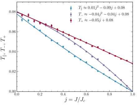
Figure 20.— The mean square of the torques (normalized to the typical (Poisson) torque $\tilde{\tau}$) as function of the angular momentum. The torques measured from static wires simulations (circles) are approximated by polynomial fits (solid lines). As expected from considerations of symmetry, for a circular orbit ($J=J_{c}$), there is no torque in the $\boldsymbol{J}$ direction and both perpendicular torques ($\tau_{b}$,$\tau_{b}$) are equal, i.e., $T_{\parallel}=T_{-}=0$. As $J\to 0$, the orbit’s geometry approaches a rod, and the torque in the $\hat{a}$ direction vanishes because its lever arm goes to zero, while the torque in the $\boldsymbol{J}$ and $\hat{b}$ directions become equal, i.e., $T_{\parallel}=T_{+}=T_{-}$.

The residual torque in the $\boldsymbol{J}$ direction is therefore

$$\sqrt{\left\langle\tau_{J}^{2}\right\rangle}/\tilde{\tau}_{N} \approx 0.28\sqrt{\left(1-j\right)\left(1-j/8\right)}\approx 0.28\sqrt{1-j}\,.$$ (D18)

This analytic fit is consistent with the Gürkan & Hopman (2007) results (fitted to $\sqrt{\left\langle\tau_{J}^{2}\right\rangle}/\tilde{\tau}_{N}\approx 0.25\sqrt{1-j^{2}}$ see Eq. (13) there) but is better, since it matches their data over the entire $j$-range. For the out-of-plane torques we obtain

$$\sqrt{\tau_{\bot}^{2}}/\tilde{\tau}_{N}\equiv\sqrt{\tau_{a}^{2}+\tau_{b}^{2}}\approx 0.28\sqrt{1-5j/8}\,.$$ (D19)

This is different from Gürkan & Hopman (2007) results (fitted to $\sqrt{\left\langle\tau_{\bot}^{2}\right\rangle}/\tilde{\tau}_{N}\approx 0.28(3/2-j^{2})$ see Eq. (14) there). However, the discrepancy can be traced to an error in their randomization procedure (Eqs. (9–11) there) which is not truly isotropic.

Using $N$-body simulations, Eilon et al. (2009) measured the isotropic averaged residual torques. They defined and measured the $j$-averaged quantities

$$\beta_{s}^{2}=\frac{Q^{2}}{N_{tot}}\left\langle\dot{J}^{2}P^{2}/J_{c}^{2}\right\rangle=4\pi^{2}\left\langle\tau_{\parallel}^{2}/\tilde{\tau}^{2}\right\rangle\,,$$ (D20)

and

$$\beta_{v}^{2}=\frac{Q^{2}}{N_{tot}}\sqrt{\left\langle\left|\dot{\mathbf{J}}\right|^{2}P^{2}/J_{c}^{2}\right\rangle}=4\pi^{2}\left\langle\left(\tau_{\parallel}^{2}+\tau_{\bot}^{2}\right)/\tilde{\tau}^{2}\right\rangle\,.$$ (D21)

Averaging the results here over $j$, we obtain $\beta_{s}\approx 1.0$ and $\beta_{v}\approx 1.7$ for $\gamma=7/4$, in agreement with Eilon et al. (2009).

Appendix E The Maximal Entropy Principle

The maximal entropy principle (MEP) has been shown to be a powerful tool in determining the steady-state (or quasi-steady-state) of dynamical systems. In particular, it was studied extensively in the context of collisionless self-gravitating systems (e.g., Lynden-Bell, 1967). Here we examine the more restricted problem of a near-Keplerian system. We prove that the RR DCs used in this study comply with the MEP. For NR, we prove that the $J$-only NR DCs comply with the MEP, since for stellar systems, the MEP is relevant only when the interactions conserve energy.

In a system where a central object of mass $M_{\bullet}$ dominates the potential (e.g., planetary systems, nuclear clusters), stars move on nearly Keplerian orbits. That is, the potential is almost regular and the orbital elements are almost constant. In particular, since the potential varies on much longer timescales than the orbital time, the potential can be orbit-averaged and the Keplerian energy is conserved.

The entropy of the system is given by

$$S=-\int d^{3}\mathbf{r}d^{3}\mathbf{v}f\left(\mathbf{r},\mathbf{v}\right)\log f\left(\mathbf{r},\mathbf{v}\right)\,,$$ (E1)

where $f$ is the stellar DF. The Keplerian energy distribution relative to the MBH, $n(E)$, is conserved

$$n\left(E;f\right)=\int d^{3}\mathbf{r}d^{3}\mathbf{v}f\left(\mathbf{r},\mathbf{v}\right)\delta\left(E-\frac{GM_{\bullet}}{r}+\frac{1}{2}v^{2}\right)\,.$$ (E2)

This implies the conservation of the total Keplerian energy $E_{\bullet}[f]=\int En\left(E;f\right)dE$ and of the total number of stars $N_{tot}\left[f\right]=\int n\left(E;f\right)dE$. Conservation of the total energy $E_{tot}=E_{\bullet}[f]+E_{\star}[f]$ then implies the conservation of the total potential energy due to the interactions with the stellar background,

$$E_{\star}[f] = \frac{1}{2}\int d^{3}\mathbf{r}\int d^{3}\boldsymbol{v}f\left(\mathbf{r},\mathbf{v}\right)\psi\left(\mathbf{r};f\right),$$ (E3)

where

$$\psi\left(\mathbf{r};f\right)=GM_{\star}\int d^{3}\mathbf{r}^{\prime}\int d^{3}\boldsymbol{v}^{\prime}\frac{f\left(\mathbf{r}^{\prime},\mathbf{v}^{\prime}\right)}{\left|\mathbf{r}-\mathbf{r}^{\prime}\right|}\,,$$ (E4)

is the star-star potential. The total angular momentum is also conserved,

$$\mathbf{L}_{tot}[f]=\int d^{3}\mathbf{r}d^{3}\mathbf{v}f\left(\mathbf{r},\mathbf{v}\right)\mathbf{L\,},$$ (E5)

where $\mathbf{L}=\mathbf{r}\times\mathbf{v}$. Using the Lagrange multipliers $\beta$, $\boldsymbol{b}$ and $\lambda(E)$, we write the target function

$$\mathcal{S} = S+\beta\left(\int d^{3}\mathbf{r}d^{3}\mathbf{v}f\left(\mathbf{r}^{\prime},\mathbf{v}^{\prime}\right)\psi\left(\mathbf{r};f\right)-2E_{\star}\right)+\mathbf{b}\cdot\left(\int d^{3}\mathbf{r}d^{3}\mathbf{v}f\left(\mathbf{r},\mathbf{v}\right)\mathbf{L}-\mathbf{L}_{tot}\right)$$

$$+\int d^{3}\mathbf{r}d^{3}\mathbf{v}f\left(\mathbf{r},\mathbf{v}\right)\lambda\left(E\right)\left(\int d^{3}\mathbf{r}^{\prime}d^{3}\mathbf{v}^{\prime}f\left(\mathbf{r}^{\prime},\mathbf{v}^{\prime}\right)\delta\left(E-\frac{GM_{\bullet}}{r^{\prime}}+\frac{1}{2}v^{\prime 2}\right)-n_{0}\left(E\right)\right)\,,$$

which is minimized by requiring

$$\frac{\delta\mathcal{S}}{\delta f} = -\log f-1+\beta\psi\left(\mathbf{r};f\right)+\mathbf{b}\cdot\boldsymbol{L}+2\lambda\left(E\right)n\left(E;f\right)=0.$$ (E7)

Therefore, the DF that maximizes the entropy is

$$f\left(\mathbf{r},\mathbf{v}\right)=A\left(E\right)e^{\beta\psi+\mathbf{b}\cdot\boldsymbol{L}}\,,$$ (E8)

where $A(E)=\exp[2\lambda(E)n(E)]$, and $\beta$ and $\boldsymbol{b}$ are constants determined by the constraints on $n(E)$, $E_{\star}$ and $\boldsymbol{L}_{tot}$. Note that an isotropic system must have $b=0$ to ensure that the DF does not depend on $\boldsymbol{L}$, and must also have $\beta=0$ since the star-star potential depends on $L$ even in an isotropic system.

E.1. Fluctuation dissipation relation for a spherical symmetric system

Since stars are assumed to move on Keplerian orbits, it is convenient to work in action-angle coordinates. Choosing the $z$-coordinate in the direction of the total angular momentum, the steady-state is

$$n\left(E,J,J_{z}\right)=n\left(E\right)\frac{e^{\beta\psi+bL_{z}}}{\int\int e^{\beta\psi+bL_{z}}dJ_{z}dJ}\,.$$ (E9)

For a spherical symmetric system with $\boldsymbol{L}_{tot}=0$, the steady-state DF is given by an implicit integral equation

$$n\left(E,J\right)=n\left(E\right)\frac{2Je^{\beta\psi(E,J,n)}}{\int e^{\beta\psi(E,J,n)}dJ^{2}}\,.$$ (E10)

MEP considerations do not require the additional assumptions that go into the FP equation (e.g., diffusion described by a Markovian process), and the MEP solution is independent of the path that the system took to reach it from its initial conditions. Therefore, the MEP solution must also be satisfied by the FP equation in steady-state, which enforces a connection between the DCs, known as the fluctuation-dissipation (F-D) relation. For the symmetries and conserved quantities of the system studied here (described by Eq. (E10)), the functional form of the F-D relation is

$$2JD_{J}e^{\beta\psi}=\frac{\partial}{\partial J}\left[JD_{JJ}e^{\beta\psi}\right].$$ (E11)

From this point on we will restrict ourselves to isotropic systems which reach a MEP solution with $\beta=0$. This is a solution of the form $n\left(E,J\right)=2n\left(E\right)J/J_{c}^{2}$. This means that DCs derived under the assumption of an isotropic background (and fixed Keplerian energy) must satisfy the F-D relation $2JD_{J}=\partial\left(JD_{JJ}\right)/\partial J$. In particular, the RR DCs that were used in this study obey this relation, as required (Bar-Or & Alexander, 2014).

E.2. Fluctuation-dissipation relation for $J$-only two-body relaxation

For NR, the coherence time is shorter than the orbital period (Section 2), and therefore orbital energy is not conserved. However, we argue in Section 3 that the flow pattern in phase-space justifies the approximate treatment of the fast $J$-diffusion as separate from the slower $E$-diffusion. We now use this property to show that in that case, the NR $J$-only DCs also satisfy the fluctuation dissipation relation, which is a partial test of the validity of the general NR DCs and is used in Section 3.

Using Eq. (LABEL:eq:DE) and setting $\Delta E=0$, we obtain

$$2v\Delta v_{\parallel}+\Delta v^{2}=0\,.$$ (E12)

Therefore, to first order in $\Delta v^{2}/v^{2}$, the local diffusion coefficients are

$$\left\langle\Delta J\right\rangle = \frac{1}{2J}\left(\frac{r^{2}}{2}-\frac{J^{2}}{v^{2}}\right)\left\langle\Delta v_{\bot}^{2}\right\rangle\,,$$ (E13)

$$\left\langle\left(\Delta J\right)^{2}\right\rangle = \frac{1}{2}\left(r^{2}-\frac{J^{2}}{v^{2}}\right)\left\langle\left(\Delta v_{\bot}\right)^{2}\right\rangle\,.$$ (E14)

The orbit-averaged diffusion coefficients are

$$D_{xy} = \left\langle\left\langle\Delta x\Delta y\right\rangle\right\rangle_{\circlearrowright}=2\int_{r_{p}}^{r_{a}}\left\langle\Delta x\Delta y\right\rangle\frac{dr}{v_{r}}\,,$$ (E15)

where $v_{r}$ is the radial velocity. Assuming a spherical potential $\Phi\left(r\right)$, the energy $E$ and angular momentum $J$ are

$$E=\frac{1}{2}v_{r}^{2}+\frac{1}{2}\left(J^{2}/r^{2}\right)+\Phi\left(r\right),$$ (E16)

and

$$J=rv_{t},$$ (E17)

where $v_{t}$ is the transverse velocity. Therefore,

$$v_{r}=\sqrt{2E-2\Phi\left(r\right)-J^{2}/r^{2}},$$ (E18)

and

$$\frac{\partial\left(1/v_{r}\right)}{\partial J}=\frac{1}{v_{r}^{2}}\frac{1}{v_{r}}\frac{J}{r^{2}}=\frac{1}{\left(r^{2}-J^{2}/v^{2}\right)}\frac{1}{v_{r}}\frac{J}{v^{2}}\,.$$ (E19)

It then follows that

$$\frac{\partial}{\partial J}\left\langle JX\right\rangle_{\circlearrowright}=\left\langle\frac{\partial}{\partial J}JX\right\rangle_{\circlearrowright}+J^{2}\left\langle\frac{X}{\left(r^{2}v^{2}-J^{2}\right)}\right\rangle_{\circlearrowright}\,,$$ (E20)

and in particular

$$\frac{1}{2J}\frac{\partial}{\partial J}JD_{JJ} = \frac{1}{2J}\left\langle\left(\frac{1}{2}r^{2}-\frac{J^{2}}{v^{2}}\right)\left\langle\left(\Delta v_{\bot}\right)^{2}\right\rangle\right\rangle_{\circlearrowright}=D_{J}\,,$$ (E21)

which therefore proves that the $J$-only NR DCs indeed satisfy the F-D relation.

References

- Alexander (2005) Alexander, T. 2005, Physics Reports, 419, 65
- Alexander (2006) —. 2006, Journal of Physics Conference Series, 54, 243
- Alexander (2010) Alexander, T. 2010, in Gravitational-wave and electromagnetic signatures of massive black hole binaries and extreme mass-ratio inspirals, ed. P. Amaro-Seoane & E. Porter (Laboratoire Astroparticule et Cosmologie, Paris), http://www.aei.mpg.de/~pau/conf_vid4/Alexander.pdf
- Alexander (2011) Alexander, T. 2011, in ASP Conf. Ser, Vol. 439, The Galactic Center: a Window to the Nuclear Environment of Disk Galaxies, ed. M. R. Morris, Q. D. Wang, & F. Yuan, 129
- Alexander (2012) Alexander, T. 2012, in European Physical Journal Web of Conferences, Vol. 39, Tidal Disruption and AGN outburst, 5001
- Alexander (2015) —. 2015, ArXiv e-prints
- Alexander & Hopman (2003) Alexander, T., & Hopman, C. 2003, ApJ, 590, L29
- Alexander & Livio (2001) Alexander, T., & Livio, M. 2001, ApJ, 560, L143
- Alexander & Morris (2003) Alexander, T., & Morris, M. 2003, ApJ, 590, L25
- Alexander & Pfuhl (2013) Alexander, T., & Pfuhl, O. 2013, in preparation
- Amaro-Seoane et al. (2007) Amaro-Seoane, P., Gair, J. R., Freitag, M., Miller, M. C., Mandel, I., Cutler, C. J., & Babak, S. 2007, Classical and Quantum Gravity, 24, 113
- Amaro-Seoane et al. (2013) Amaro-Seoane, P., Sopuerta, C. F., & Freitag, M. D. 2013, MNRAS, 429, 3155
- Antonini (2014) Antonini, F. 2014, ApJ, 794, 106
- Antonini & Merritt (2013) Antonini, F., & Merritt, D. 2013, ApJ, 763, L10
- Bahcall & Wolf (1976) Bahcall, J. N., & Wolf, R. A. 1976, ApJ, 209, 214
- Bar-Or & Alexander (2014) Bar-Or, B., & Alexander, T. 2014, Classical and Quantum Gravity, 31, 244003
- Bar-Or et al. (2013) Bar-Or, B., Kupi, G., & Alexander, T. 2013, ApJ, 764, 52
- Binney & Tremaine (2008) Binney, J., & Tremaine, S. 2008, Galactic Dynamics: Second Edition (Princeton University Press)
- Brem et al. (2014) Brem, P., Amaro-Seoane, P., & Sopuerta, C. F. 2014, MNRAS, 437, 1259
- Chandrasekhar (1944) Chandrasekhar, S. 1944, ApJ, 99, 47
- Cohn (1979) Cohn, H. 1979, ApJ, 234, 1036
- Cohn & Kulsrud (1978) Cohn, H., & Kulsrud, R. M. 1978, ApJ, 226, 1087
- Eilon et al. (2009) Eilon, E., Kupi, G., & Alexander, T. 2009, ApJ, 698, 641
- Ferrarese & Merritt (2000) Ferrarese, L., & Merritt, D. 2000, ApJ, 539, L9
- Frank & Rees (1976) Frank, J., & Rees, M. J. 1976, MNRAS, 176, 633
- Freitag (2001) Freitag, M. 2001, Classical and Quantum Gravity, 18, 4033
- Freitag (2003) —. 2003, ApJ, 583, L21
- Gair et al. (2006) Gair, J. R., Kennefick, D. J., & Larson, S. L. 2006, ApJ, 639, 999
- Gebhardt et al. (2000) Gebhardt, K., et al. 2000, ApJ, 539, L13
- Ghez et al. (2003) Ghez, A. M., et al. 2003, ApJ, 586, L127
- Gillessen et al. (2009a) Gillessen, S., Eisenhauer, F., Trippe, S., Alexander, T., Genzel, R., Martins, F., & Ott, T. 2009a, ApJ, 692, 1075
- Gillessen et al. (2009b) Gillessen, S., et al. 2009b, ApJ, 692, 1075
- Goodman (2003) Goodman, J. 2003, MNRAS, 339, 937
- Gürkan & Hopman (2007) Gürkan, M. A., & Hopman, C. 2007, MNRAS, 379, 1083
- Hamers et al. (2014) Hamers, A. S., Portegies Zwart, S. F., & Merritt, D. 2014, MNRAS, 443, 355
- Heggie & Hut (2003) Heggie, D., & Hut, P. 2003, The Gravitational Million-Body Problem: A Multidisciplinary Approach to Star Cluster Dynamics (Cambridge University Press, 2003, 372 pp.)
- Hills (1988) Hills, J. G. 1988, Nature, 331, 687
- Hils & Bender (1995) Hils, D., & Bender, P. L. 1995, ApJ, 445, L7
- Hopman & Alexander (2005) Hopman, C., & Alexander, T. 2005, ApJ, 629, 362
- Hopman & Alexander (2006a) —. 2006a, ApJ, 645, 1152
- Hopman & Alexander (2006b) —. 2006b, ApJ, 645, L133
- Ivanov (2002) Ivanov, P. B. 2002, MNRAS, 336, 373
- Kocsis & Tremaine (2015) Kocsis, B., & Tremaine, S. 2015, MNRAS, 448, 3265
- Lightman & Shapiro (1977) Lightman, A. P., & Shapiro, S. L. 1977, ApJ, 211, 244
- Lynden-Bell (1967) Lynden-Bell, D. 1967, MNRAS, 136, 101
- Lyne et al. (2004) Lyne, A. G., et al. 2004, Science, 303, 1153
- Madigan et al. (2011) Madigan, A.-M., Hopman, C., & Levin, Y. 2011, ApJ, 738, 99
- Magorrian & Tremaine (1999) Magorrian, J., & Tremaine, S. 1999, MNRAS, 309, 447
- Merritt (2015a) Merritt, D. 2015a, ApJ, 804, 52
- Merritt (2015b) —. 2015b, ApJ, 804, 128
- Merritt et al. (2010) Merritt, D., Alexander, T., Mikkola, S., & Will, C. M. 2010, Phys. Rev. D, 81, 062002
- Merritt et al. (2011) —. 2011, Phys. Rev. D, 84, 044024
- Miralda-Escudé & Gould (2000) Miralda-Escudé, J., & Gould, A. 2000, ApJ, 545, 847
- Nelson & Tremaine (1999) Nelson, R. W., & Tremaine, S. 1999, MNRAS, 306, 1
- Ostriker (1983) Ostriker, J. P. 1983, ApJ, 273, 99
- Perets et al. (2008) Perets, H. B., Gualandris, A., Merritt, D., & Alexander, T. 2008, in The Central Kiloparsec: Active Galactic Nuclei and Their Hosts (Memorie della Societa Astronomica Italiana), in press
- Perets et al. (2007) Perets, H. B., Hopman, C., & Alexander, T. 2007, ApJ, 656, 709
- Peters (1964) Peters, P. C. 1964, Physical Review, 136, 1224
- Peters & Mathews (1963) Peters, P. C., & Mathews, J. 1963, Physical Review, 131, 435
- Rauch & Tremaine (1996) Rauch, K. P., & Tremaine, S. 1996, New Astronomy, 1, 149
- Rees (1988) Rees, M. J. 1988, Nature, 333, 523
- Risken (1989) Risken, H. 1989, The Fokker-Planck equation. Methods of solution and applications
- Shapiro & Marchant (1978) Shapiro, S. L., & Marchant, A. B. 1978, ApJ, 225, 603
- Sigurdsson (2003) Sigurdsson, S. 2003, Classical and Quantum Gravity, 20, 45
- Sigurdsson & Rees (1997) Sigurdsson, S., & Rees, M. J. 1997, MNRAS, 284, 318
- Syer & Ulmer (1999) Syer, D., & Ulmer, A. 1999, MNRAS, 306, 35
- Touma et al. (2009) Touma, J. R., Tremaine, S., & Kazandjian, M. V. 2009, MNRAS, 394, 1085
- Will (2006) Will, C. M. 2006, Living Reviews in Relativity, 9, 3
- Young et al. (1977) Young, P. J., Shields, G. A., & Wheeler, J. C. 1977, ApJ, 212, 367