Campbell penetration in the critical state of type II superconductors

Abstract

The penetration of an $ac$ magnetic signal into a type II superconductor residing in the Shubnikov phase depends on the pinning properties of Abrikosov vortices. Within a phenomenological theory, the so-called Campbell penetration depth $\lambda_{\rm\scriptscriptstyle C}$ is determined by the curvature $\alpha$ at the bottom of the effective pinning potential. Preparing the sample into a critical state, this curvature vanishes and the Campbell length formally diverges. We make use of the microscopic expression for the pinning force density derived within strong pinning theory and show how flux penetration on top of a critical state proceeds in a regular way.

I Introduction

Transport onnes_11 and magnetization meissner_33 measurements are well known tools for the basic phenomenological characterization of superconductors. The diamagnetic screening in a superconductor involves multiple aspects: a weak magnetic field penetrates to the material over the length $\lambda_{\rm\scriptscriptstyle L}$, the (London) penetration depth london_35 , which provides access to the superfluid density $\rho_{s}$ and is typically of sub-micrometer size. In type II superconductors, a magnetic field $H$ penetrates the material through quantized flux-lines or Abrikosov vortices abrikosov_57 which arrange in a triangular lattice defining the Shubnikov phase shubnikov_37 . Testing this phase via a small $ac$-magnetic field produces a normal response described by the skin-effect, with a reduced (flux-flow) resistivity $\rho_{\mathrm{ff}}$ entering the usual expression for the skin-depth $\delta(\omega)$. In real materials, vortices get pinned by material defects, thereby establishing the desired critical current density $j_{c}$ below which vortices are trapped. In this situation, an external $ac$-field probes the pinning landscape (or pinscape), as the latter now determines the field penetration over the scale $\lambda_{\mathrm{\scriptscriptstyle C}}$ (typically $1$ – $100$ micrometers), the Campbell lengthcampbell_69 . The linear response in the Campbell regime assumes that the vortex displacements induced by the $ac$-magnetic field $h_{ac}$ are much smaller than the characteristic pinning length such that the Campbell response probes the pinning wells. This condition implies that the currents $\delta j\sim ch_{ac}/\lambda_{\mathrm{\scriptscriptstyle C}}$ induced by the vortex displacements are much smaller than the system’s critical current $j_{c}$, $\delta j\ll j_{c}$. Increasing the field strength $h_{ac}$ to large values capable of changing the direction of the critical state periodically, i.e., $\delta j>j_{c}$, the response is described by the Bean modelbean_62 . In this limit, the Bean penetration depth $\ell_{\mathrm{\scriptscriptstyle B}}\sim ch_{ac}/4\pi j_{c}$ depends on the field amplitude $h_{ac}$ and hence generates a higher harmonic signal in the magnetic response.

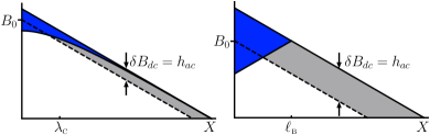
Figure 1: Sketch of the linear Campbell (left panel) vs. non-linear Bean (right panel) response of a vortex critical state subject to an $ac$ magnetic field $h_{ac}$. The gray-shaded areas show the change of the $dc$ field deep inside the sample after the initial field penetration at short times. The blue regions indicate the magnetic field oscillations at large times penetrating the sample to the depths $\lambda_{\mathrm{\scriptscriptstyle C}}$ and $\ell_{\mathrm{\scriptscriptstyle B}}$, respectively. The cross-over between the Campbell- and Bean regimes with increasing field amplitude $h_{ac}$ occurs when the induced current $\delta j$ near the sample surface is of the order of $j_{c}$, i.e., when $h_{ac}\gtrsim j_{c}\lambda_{\mathrm{\scriptscriptstyle C}}/c$.

Within a phenomenological model of the Campbell response, the dynamics of vortices in a random potential landscape is reduced to the motion of a vortex in an effective defect potential. Vortices probe the bottom of the pinning potential and the Campbell penetration depth $\lambda_{\rm\scriptscriptstyle C}\propto 1/\sqrt{\alpha}$ involves the curvature $\alpha$ at the minimum of the effective pinning well campbell_69 . This description becomes quite problematic when dealing with the technologically most relevant vortex configuration, the critical state bean_62 realizing the maximally possible current flow (the critical current density $j_{c}$) before depinning. Indeed, within this approach, the critical state is characterized by a vanishingprozorov_03 curvature $\alpha(j)\propto(j_{c}-j)^{1/2}\to 0$ and thus implies a diverging Campbell length $\lambda_{\rm\scriptscriptstyle C}$. This result is not satisfactory in two respects: first, the predicted divergence is not observed in experiments prozorov_03 ; an explanation that flux creep prevents probing of the proper critical state is hardly applicable to the early work by Campbellcampbell_69 on low-$T_{c}$ Pb-Bi alloys. Second, it turns out that the Campbell length in the critical state can be even smaller than that in the field-cooled stateprozorov_13 ; willa_15b .

In this paper, we make use of a microscopic theory in order to reconcile the apparent divergence of the penetration depth $\lambda_{\rm\scriptscriptstyle C}\propto 1/\sqrt{\alpha}$ in the critical state with a regular vortex dynamics. To this end, we describe the $ac$-magnetic penetration within the strong pinning framework willa_15b and determine the dynamical evolution of the vortex state when probing a critical state with a small-amplitude and low-frequency $ac$-magnetic field $h_{ac}e^{-i\omega t}$. We show that in this situation the $ac$-response involves a transient region where vortices first penetrate throughout the sample in the form of diffusive flux pulses. The penetrated flux produces an upward shift of the critical state profile; once this $dc$ shift reaches the maximal field amplitude $h_{ac}$, see Fig. 1 (left), the $ac$-field only lowers the magnetic field at the sample edge and we arrive at a finite $ac$ penetration depth $\lambda_{\rm\scriptscriptstyle C}\propto 1/\sqrt{\Delta f_{\mathrm{pin}}}$, with $\Delta f_{\mathrm{pin}}$ the jump in the microscopic pinning force for the critical state as given by the strong pinning theory. While, qualitatively, a similar picture describes the non-linear $ac$ response at large field amplitudes $h_{ac}>j_{c}\lambda_{\rm\scriptscriptstyle C}/c$ as described by the Bean modelbean_62 and illustrated in the right panel of Fig. 1, the quantitative description and results are very different for the Campbell and Bean penetration regimes.

In the following, we briefly review (Sec. II) the $ac$-magnetic response of a type II superconductor in the Shubnikov phase and its microscopic extension using the result from strong pinning theory. In Section III we describe the transient regime of the $ac$-response with its vortex penetration, the central topic of this paper. Section IV gives a short summary and conclusions.

II $ac$ Response and Campbell Length

An $ac$ dynamical field enters a homogeneous metallic sample over the skin-depth $\delta(\omega)\approx\sqrt{c^{2}/2\pi\mu\omega\sigma}$, with $\mu$ and $\sigma$ the materials’ magnetic permeability and conductivity, respectively. For the inhomogeneous state of a field-penetrated type II superconductor, it is the behavior of vortices which determines the $ac$ response. In a real, i.e., defected material, the dynamics of pinned vortices is dictated by the pinning potential opposing their motion; within a phenomenological model, the force density $F_{\mathrm{pin}}\approx-\alpha x$ defines the penetration depth $\lambda_{\rm\scriptscriptstyle C}$ at small frequencies $\omega$,

$$\lambda_{\rm\scriptscriptstyle C}^{2}=\frac{B^{2}}{4\pi\alpha},$$ (1)

where $B$ is the mean penetrated field. The above result for $\lambda_{\rm\scriptscriptstyle C}$ was first given by Archie Campbell campbell_69 , together with supporting experimental data on the $ac$-magnetic response of a superconductor.

For a brief derivation of the result (1), we consider a superconductor occupying the half-space $X>0$ in the presence of a magnetic field involving both $dc$ and (a small) $ac$ component $H(t)=H_{0}+h_{ac}\exp(-i\omega t)$ directed along $Z$ (for consistency with Ref. willa_15b, we use capital-letter coordinates in describing the macroscopic situation). This field penetrates to the sample in the form of vortices producing an average magnetic induction $B(X,t)$. The screening current density $j$ in the superconductor flows along the $Y$-axis and exerts a Lorentz force density $F_{\rm\scriptscriptstyle L}=jB/c$ directed into the sample. In a stationary state, the Lorentz force density $F_{\rm\scriptscriptstyle L}$ has to be balanced by the pinning force density $F_{\mathrm{pin}}$, otherwise vortices move dissipatively. Introducing the macroscopic displacement field $U(X,t)$ of the vortex system, the force balance equation takes the form

$$\eta\partial_{t}U=F_{\rm\scriptscriptstyle L}(j,U)+F_{\mathrm{pin}}(X,U),$$ (2)

with $\eta$ denoting the viscosity bardeen_65 . The magnetic induction and current can be split into a $dc$ part and a contribution from the external $ac$ drive, $B(X,t)=B_{0}+\delta B(X,t)$ and $j(X,t)=j_{0}+\delta j(X,t)$, where $B$ is driven at the boundary, $B(0,t)=B_{0}+h_{ac}\exp(-i\omega t)$. The $ac$-magnetic induction $\delta B$ relates to $\delta j$ via Ampère’s law, $\partial_{\rm\scriptscriptstyle X}\delta B=-(c/4\pi)\delta j$, and to the displacement $U$ via the change in vortex density, $\delta B/B_{0}\approx-\partial_{\scriptscriptstyle X}U$. For a critical state, the $dc$ current density $j_{0}$ is maximal and hence equals the critical current density $j_{c}$. The latter is compensated by the maximal (or critical) pinning force density $\max F_{\mathrm{pin}}=-F_{c}$, with $F_{c}=j_{c}B/c$. Rewriting the Lorentz force density through $U$ and denoting deviations from maximal pinning by $\delta F_{\mathrm{pin}}\equiv F_{c}-F_{\mathrm{pin}}(U)$, we arrive at the dynamical equation of the form,

$$\eta\partial_{t}U-(B_{0}^{2}/4\pi)\partial^{2}_{\scriptscriptstyle X}U-\delta F_{\mathrm{pin}}(U)=0,$$ (3)

Alternatively, this equation can be obtained starting from the equation of motion of individual vortices. Averaging over many inter-vortex spacings $a_{0}$, one then arrives at the above expression. With the chosen field and current directions, the vortex-vortex interaction [second term in Eq. (3)] only involves the bulk compression modulus $c_{11}(\boldsymbol{k}=0)=B_{0}^{2}/4\pi$, while contributions of the shear and tilt moduli are averaged to zero.

The non-trivial part in arriving at an explicit equation for $U(X,t)$ is the functional dependence of the pinning force density $\delta F_{\mathrm{pin}}(U)$. Assuming vortices trapped in a harmonic pinning potential, Campbell campbell_69 introduced the phenomenological Ansatz $\delta F_{\mathrm{pin}}(U)=-\alpha U$, with $\alpha$ describing the curvature of the effective pinning potential. The resulting differential equation is of the driven-diffusive type and easily solved,

$$U(X,t) =\lambda_{\rm\scriptscriptstyle C}(h_{ac}/B_{0})e^{-X/\lambda_{\rm\scriptscriptstyle C}}e^{-i\omega t}$$ (4)

with

$$\lambda_{\rm\scriptscriptstyle C}^{2}(\omega) =\frac{B_{0}^{2}}{4\pi}\frac{1}{\alpha-i\omega\eta}.$$ (5)

At small frequencies, we obtain the Campbell length $\lambda_{\rm\scriptscriptstyle C}=\lambda_{\rm\scriptscriptstyle C}(\omega=0)$ as given in Eq. (1); at high frequencies we make use of the Bardeen formula $\eta=BH_{c2}/c^{2}\rho_{n}$ to arrive at the skin depth $\delta(\omega)\approx(c^{2}/2\pi\omega\sigma_{\mathrm{ff}})^{1/2}$ with $\sigma_{\mathrm{ff}}=\sigma_{n}H_{c2}/B$ the flux flow conductivity, $\sigma_{n}$ the normal state conductivity, $H_{c2}=\Phi_{0}/2\pi\xi^{2}$ the upper critical field, and $\xi$ the coherence length of the superconductor.

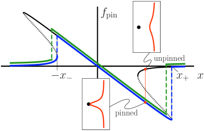
Figure 2: Microscopic effective pinning force $f_{\mathrm{pin}}$ with bistable pinned and unpinned solutions as a function of the pin-vortex distance $x$ (dotted lines denote unstable solutions). For randomly positioned defects and the vortex lattice in the critical state, the occupation of the force branches (blue) produces the maximal restoring force $F_{\mathrm{pin}}=n_{p}\langle f_{\mathrm{pin}}\rangle=-F_{c}$. A macroscopic displacement $U>0$ of all vortices in the direction of the Lorentz force does not change the branch occupation and $\delta F_{\mathrm{pin}}=0$. A displacement $U<0$ against the Lorentz force, however, modifies the branch occupation (green) and reduces the pinning force $\delta F_{\mathrm{pin}}\propto\Delta f_{\mathrm{pin}}U$, see Eq. (7).

Here, we go beyond this phenomenological theory and make use of the expression for the restoring force $\delta F_{\mathrm{pin}}$ derived from strong pinning theory willa_15b . The latter goes back to early work of Labusch labusch_69 and of Larkin and Ovchinnikov larkin_79 and has attracted quite some interest over the recent years blatter_04 ; koshelev_11 ; thomann_12 . Within the framework of strong pinning theory, vortices are pinned by individual defects, thus allowing for a quantitative description of pinning related phenomena. The crucial feature appearing within strong pinning is the strong deformation of vortices giving rise to bistable solutions of the force equation balancing the elastic vortex energy against the pinning energy due to the defect; the appearance of such bistable solutions, quantitatively formulated in the Labusch criterionlabusch_69 $\kappa=1$, then separates strong ($\kappa>1$) from weak ($\kappa<1$) pinning (the Labusch parameter $\kappa\sim f_{p}/\bar{C}\xi$ measures the relative strength of the pinning force $f_{p}$ of one defect as compared to an effective elasticity $\bar{C}$ of the vortex lattice).

Within strong pinning theory, one studies how a representative vortex embedded in the vortex lattice gets locally deformed and pinned due to the presence of a defect willa_15b ; the macroscopic pinning force density $F_{\mathrm{pin}}$ then results from proper averaging of the microscopic effective pinning force $f_{\mathrm{pin}}$. More specifically, when dragging a vortex across an individual defect, the vortex jumps into the pinning potential at $-x_{-}$, $x_{-}\sim\xi$, and remains pinned therein until the deformation becomes too large and the vortex snaps out of the pin at $x_{+}\sim\kappa\xi$, see Fig. 2. Assuming a small density $n_{p}$ of pinning centers, one can ignore interactions between defects and the pinning force density $F_{\mathrm{pin}}=n_{p}\langle f_{\mathrm{pin}}\rangle$ derives from a simple average over the microscopic pinning states with vortices occupying pinned and unpinned branches of the bistable pinning landscape. A vortex system in the (Bean) critical state is defined through the maximal averaged pinning force density $F_{c}$ produced by the pins. In this state, the vortex configuration is critical, i.e., when shifting the vortex system in the direction of vortex penetration $U>0$ there is no change in pinning force as the latter is already maximal,

$$\delta F_{\mathrm{pin}}(U>0)=0.$$ (6)

On the other hand, moving vortices opposite to the critical slope, i.e., for $U<0$, the branch occupation rearranges, see Fig. 2, and the pinning force density is diminished by willa_15b

$$\delta F_{\mathrm{pin}}(U<0) \approx-n_{p}(t_{\perp}/a_{0}^{2})\Delta f_{\mathrm{pin}}\,U.$$ (7)

Here, $\Delta f_{\mathrm{pin}}$ denotes the sum of jumps in the pinning force when vortices jump into and snap out of the pinning trap created by a defect. Furthermore, $t_{\perp}$ is the transverse length over which vortices passing by the defect are trapped and $a_{0}^{-2}=B/\Phi_{0}$ is the vortex density ($\Phi_{0}=hc/2e$ denotes the flux unit). For a point-like defect, the transverse trapping length is of the order of the vortex core size, $t_{\perp}\sim\xi$.

The drop (7) in critical force appears whenever vortices start moving to the left, i.e., when $U(X,t)$ decreases with increasing $t$. In the dynamical situation defined by the $ac$-response, we have to follow the macroscopic displacement $U(X,t)$ in time and switch on the restoring force (7) when $U$ starts decreasing. Assume that vortices have reached the displacement $U_{0}$ when they change direction of motion; the argument in Eq. (7) then has to be replaced by $U-U_{0}$, with the restoring force smoothly growing from zero. In a fully dynamical situation, $U_{0}$ has to be calculated self-consistently and is given by the maximal displacement reached so far, $U_{0}(X,t)=\max_{t^{\prime}<t}U(X,t^{\prime})$. The final expression for the reduction in pinning force then is given by

$$\delta F_{\mathrm{pin}}(U) =-\alpha_{\mathrm{sp}}\,(U-U_{0})$$ (8)

with

$$\alpha_{\mathrm{sp}} \approx n_{p}(t_{\perp}/a_{0}^{2})\Delta f_{\mathrm{pin}}.$$ (9)

In the following, we solve the dynamical equation for $U(X,t)$, Eq. (3), with the restoring force $\delta F_{\mathrm{pin}}$, Eq. (8), derived from strong pinning theory.

III Critical State $ac$-Response

Before entering the detailed discussion we give a short overview on the $ac$ dynamics. Inserting the result (8) into Eq. (3) generates a complex vortex dynamics as flux enters the sample in a sequence of diffusive pulses until the internal magnetic field is raised to $B_{0}+h_{ac}$—the discussion of this initial dynamics is the central topic of the paper carried out below. Once the asymptotic time domain has been reached, vortices exhibit the typical oscillatory behavior within the pinning wells, but with respect to the new critical state that has been shifted upward by $h_{ac}$, see Sec. III.2 below. The $ac$ magnetic response then follows the standard result with the Campbell length $\lambda_{\rm\scriptscriptstyle C}$ determined by the jump in pinning force $\Delta f_{\mathrm{pin}}$ through $\alpha_{\mathrm{sp}}$, see Eq. (9).

III.1 Transient initialization regime

Our task is to solve the boundary-driven differential equation

$$-\partial_{t}U+D\partial_{\scriptscriptstyle X}^{2}U-\frac{\alpha_{\mathrm{sp}}}{\eta}(U-U_{0})=0$$ (10)

with the diffusion constant $D=B_{0}^{2}/4\pi\eta$, the max-field $U_{0}(X,t)=\max_{t^{\prime}<t}U(X,t^{\prime})$, and the external drive $\partial_{\scriptscriptstyle X}U(0,t)=-(h_{ac}/B_{0})e^{-i\omega t}$. In a sample of finite thickness $d$ along $X$ vortices cannot move beyond the sample center, hence $U(d/2,t)=0$ provides the second boundary condition. We consider a situation where the magnetic field $B_{0}$ changes little over the critical state profile, e.g., as it is the case for a fully penetrated sample with thickness $d\ll L$, $L=cB_{0}/4\pi j_{c}$ the asymptotic extension of the critical state profile, $B(X)=B_{0}(L-X)/L$.

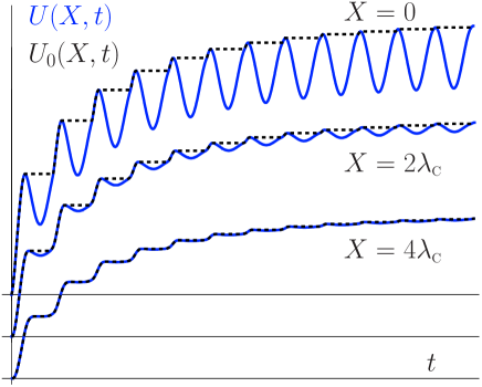
Figure 3: Displacement $U$ (solid, blue) and max-field $U_{0}$ (black, dashed) as a function of time $t$ at the positions $X=0$ (sample boundary), $X=2\lambda_{\rm\scriptscriptstyle C}$, and $X=4\lambda_{\rm\scriptscriptstyle C}$ (subsequent curves are shifted for better visibility). The periodic decrease in $U$ describes relaxation of vortices in the pinning wells. With the max-field $U_{0}$ remaining constant over these regions, a reduction $\delta F_{\mathrm{pin}}$ in pinning force density below $F_{c}$ shows up.

Consider first the driven diffusion equation without the pinning term. The (asymptotic) solution of this equation has the form $U(X,t)=(h_{ac}/B_{0})e^{-(1-i)(X/\delta)}e^{-i\omega t}$ with $\delta$ the skin depth involving the flux-flow conductivity; the displacement $U(0,t)$ at the boundary describes the net flux (per unit length along $Y$) $\phi(t)=B_{0}U(0,t)$ that has entered the sample up to time $t$—obviously flux periodically enters and leaves the sample as well known from the skin effect.

The pinning force term $-\alpha_{\mathrm{sp}}(U-U_{0})$ breaks the symmetry between vortices moving in and out of the sample. While flux entry proceeds as before, flux exit is inhibited as the pinning force pushes the vortices into the sample (due to the reduction of the critical force). As a result, flux is periodically pumped into the sample until the total additional flux reaches a value $\phi=h_{ac}d/2$ and the internal magnetic field is shifted from $B_{0}$ to $B_{0}+h_{ac}$.

The differential equation for the displacement field $U(X,t)$ as well as the max-field $U_{0}(X,t)$ can be found by numerical integration of Eq. (10). To this end, we bring Eq. (10) into a dimensionless form by measuring the time in units of the period $\tau=2\pi/\omega$ and lengths (and displacements) in units of the typical diffusion length $\ell_{D}=\sqrt{D\tau}$ during the period $\tau$. The differential equation (10) then assumes the form

$$-\partial_{t}U+\partial_{\scriptscriptstyle X}^{2}U-\frac{\ell_{D}^{2}}{\lambda_{\mathrm{\scriptscriptstyle C}}^{2}}(U-U_{0})=0,$$ (11)

with $t$, $X$, $U$, and $U_{0}$ the new dimensionless quantities and $\lambda_{\rm\scriptscriptstyle C}=\sqrt{D\eta/\alpha_{\mathrm{sp}}}=\sqrt{B_{0}^{2}/4\pi\alpha_{\mathrm{sp}}}$ the strong pinning result for the Campbell length. The boundary condition at the surface $X=0$ now reads $\partial_{X}U(0,t)=-(h_{ac}/B_{0})e^{-i2\pi t}$, while the vanishing of the displacement at the sample center, $U(d/2\ell_{D},t)=0$, inhibits vortices from further penetrating the sample. The relative amplitude $(h_{ac}/B_{0})$ trivially scales the solution, while the ratios $\lambda_{\mathrm{\scriptscriptstyle C}}/\ell_{D}$ and $d/2\ell_{D}$ determine the shape of the solution for a specific setup. The algorithm to solve Eq. (11) is based on the forward Euler routine on a discrete mesh with spacing $\Delta X$ ($\Delta t$) in the spacial (time) domain. The standard scheme

$$U(X,t+\Delta t) =U(X,t)+\frac{\Delta t}{(\Delta X)^{2}}\big{[}U(X-\Delta X,t)-2U(X,t)+U(X+\Delta X,t)\big{]}-\frac{\ell_{D}^{2}\Delta t}{\lambda_{\mathrm{\scriptscriptstyle C}}^{2}}[U(X,t)-U_{0}(X,t)],$$ (12)

has to be supplemented with an update of the max-field

$$U_{0}(X,t+\Delta t) =\max\{U(X,t+\Delta t),U_{0}(X,t)\}.$$ (13)

This additional rule does not allow for more advanced numerical approaches such as the implicit Crank-Nicolson method. The physical constraint to resolve the dynamics within the Campbell length $(\Delta X)^{2}\ll(\lambda_{\mathrm{\scriptscriptstyle C}}/\ell_{D})^{2}$ sets a lower bound for $\Delta X$. The requirement of good convergence of the numerical code imposes a constraint on the mesh size $\Delta t$ via $\Delta t/(\Delta X)^{2}\ll 1$ [these two constraints also guarantee that $\ell_{D}^{2}\Delta t/\lambda_{\mathrm{\scriptscriptstyle C}}^{2}\ll 1$, see Eq. (12)]. A second constraint on the time mesh $\Delta t\ll 1$, guaranteeing the smoothness of the external drive, is automatically satisfied for the parameter range considered here. The results shown in Figs. 3 – 5 assume $\lambda_{\mathrm{\scriptscriptstyle C}}/\ell_{D}=1/\sqrt{20\pi}\approx 1/8$ and $d/2\ell_{D}=1$. In Fig. 6 different system sizes $d/2\ell_{D}=$ 1, 3, 5, 7, and 9 are shown.

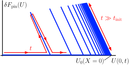
Figure 4: Change in pinning force density $\delta F_{\mathrm{pin}}$ versus displacement field $U$ at the sample surface $X=0$. The time $t$ is a curve parameter that evolves as indicated by the red line. Starting from $U=0$ and increasing $U$, flux moves into the sample, the pinning force density is at its maximum value $F_{\mathrm{pin}}=-F_{c}$, and $\delta F_{\mathrm{pin}}=0$. Deviations of $F_{\mathrm{pin}}$ from its critical value appear whenever $U$ decreases and vortices relax in their pinning potential. At long times, the Bean profile has been raised to the value $B_{0}+h_{ac}$ and vortices oscillate reversibly (see double-headed red arrow) within their potential wells without additional flux entrance and vanishing regions with $\delta F_{\mathrm{pin}}=0$. The max-field $U_{0}(0,t)$ reaches its asymptotic value $U_{0}(X=0)$, see Eq. (24).

The displacement fields $U(X,t)$ and $U_{0}(X,t)$ are shown in Fig. 3 for several positions $X$, once at the boundary $X=0$ where $U$ is proportional to the penetrated flux $\phi$ (per unit length along $Y$), as well as a few penetration depths $\lambda_{\rm\scriptscriptstyle C}$ into the sample at $X=2\lambda_{\rm\scriptscriptstyle C}$ and $X=4\lambda_{\rm\scriptscriptstyle C}$. Due to the action of the pinning force term, the displacement $U$ is no longer periodic: the increase in $U$ describing flux entry is interrupted by short excursions with decreasing $U$ as vortices relax in their pinning potential. The max-field $U_{0}$ ignores these depressions and the finite amplitude $U_{0}-U$ generates the decrease in pinning force $\delta F_{\mathrm{pin}}$. The latter is shown in Fig. 4: Regions of vanishing $\delta F_{\mathrm{pin}}$ where additional flux penetrates deeper into the sample are interrupted by segments of finite force $\delta F_{\mathrm{pin}}>0$ where vortices relax back in their pinning potentials. With increasing time, the additional flux shifts the internal field upwards to $B_{0}+h_{ac}$. For long times, vortices evolve reversibly within their pinning wells, with no further flux entering the sample. As a result, the change in pinning force density $\delta F_{\mathrm{pin}}$ oscillates back and forth with maximal amplitude and no intermediate regions with $\delta F_{\mathrm{pin}}=0$ show up.

The physically most relevant and transparent result is the behavior of the magnetic induction $B$ within the sample. In Fig. 5 we show the evolution of $\delta B(X,t)$ with time $t$ over several penetration depths into the sample along $X$. Additional flux is periodically pumped into the sample, lifting the $dc$ value of $B$ with increasing time $t$ (change from green to blue color). For better illustration we have chosen a geometry and parameters such that the 8 cycles shown in the figure nearly suffice to reach the asymptotic value $B_{0}+h_{ac}$, see also the lowest curve in Fig. 6 for $d/2\ell{D}=1$.

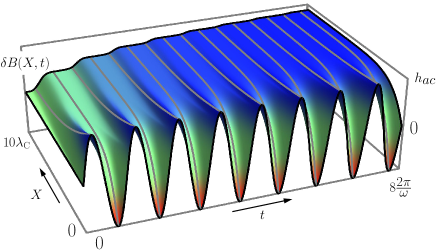
Figure 5: Change in magnetic induction $\delta B(X,t)$ as a function of time $t$ and distance $X$ into the sample. Every oscillation pumps flux into the sample, pushing the critical state at $B_{0}$ ($\delta B=0$, green) towards one at $B_{0}+h_{ac}$ ($\delta B=h_{ac}$, blue). The 8 cycles shown here push almost all the flux into the sample that is required for its shift by $h_{ac}$.

In the following, we build and analyze a simple model for the flux entry into the sample; this will allow us to estimate the number of cycles needed to reach the asymptotic state. We start with the first $ac$ cycle which pumps a flux (per unit transverse length) $\phi_{0}=f\,h_{ac}\ell_{D}$ into the sample, where $\ell_{D}=\sqrt{D\tau}$ is the diffusion length during one cycle, $\tau=2\pi/\omega$, and $f<1$ is a numerical factor accounting for the magnitude of penetrated flux per pulse (note that flux is pumped into the sample only during the first half-cycle and the precise magnitude depends on the detailed shape of the driving signal). This flux pulse diffuses with time $t$ and spreads over the distance $\sqrt{Dt}$. At time $t$, the flux pulse then reduces the $ac$-magnetic field amplitude at the sample boundary $X=0$ by $\bar{h}_{0}(t)=\phi_{0}/\sqrt{Dt}$. Hence the next pulse $\phi_{1}$ entering the sample is reduced, $\phi_{1}=f\,[h_{ac}-\bar{h}_{0}(\tau)]\ell_{D}$. Iterating this process, the $i$-th flux pulse entering the sample is given by

$$\phi_{i}=f\,h_{i}\ell_{D},$$ (14)

with the iteratively defined amplitude

$$h_{i}=h_{ac}-\sum_{m<i}\bar{h}_{m}(i\tau)$$ (15)

and

$$\bar{h}_{m}(t)=\phi_{m}/\sqrt{D(t-m\tau)}.$$ (16)

Combining Eqs. (14), (15), and (16) we then have to solve the self-consistency equation for $h_{i}$,

$$h_{i}=h_{ac}-f\sum_{m<i}\frac{h_{m}}{\sqrt{i-m}}.$$ (17)

Going over to continuous variables, we obtain the integral equation

$$h(t)=h_{ac}-\frac{f}{\sqrt{\tau}}\int_{t_{0}}^{t}dt^{\prime}\frac{h(t^{\prime})}{\sqrt{t-t^{\prime}}},$$ (18)

with the starting time $t_{0}$ to be determined together with $h(t)$. Inserting the Ansatz $h(t)=\beta\,h_{ac}/\sqrt{t}$, we can carry out the integral and arrive at the self-consistency condition

$$\beta\,\frac{h_{ac}}{\sqrt{t}}=h_{ac}\bigg{[}1-\frac{2f\beta}{\sqrt{\tau}}\arcsin\big{(}\sqrt{t^{\prime}/t}\big{)}\Big{|}_{t_{0}}^{t}\bigg{]}.$$ (19)

Choosing $\beta=\sqrt{\tau}/f\pi$ (such that the upper boundary $t$ provides a term $(2/\pi)\arcsin 1=1$) and setting $t_{0}=\tau/2f^{2}$, we obtain a consistent solution for large timesfootnote2 $t\gg t_{0}$ in the form

$$h(t)=\frac{h_{ac}}{f\pi}\sqrt{\frac{\tau}{t}}.$$ (20)

Finally, adding up the flux pulses $\phi_{i}$, we find that the flux penetrates into the sample diffusively as

$$\phi(t)=\frac{2}{\pi}h_{ac}\ell_{D}\sqrt{t/\tau},$$ (21)

independent on $f$. The flux needed to push the internal critical state from an initial field $B_{0}d/2$ to a final field $(B_{0}+h_{ac})d/2$ then involves the time

$$t_{\mathrm{init}}=\frac{\pi^{2}}{16}\frac{d^{2}}{\ell_{D}^{2}}\tau$$ (22)

or $n=(\pi^{2}/16)\,d^{2}/\ell_{D}^{2}$ cycles. In Fig. 6 we compare the result of our analytic model calculation with our numerical data. For the latter, we have computed the response of the vortex system for different system sizes with the thickness $d/2$ of the critical state profile taking the values $d/2\ell_{D}=$ 1, 3, 5, 7, and 9 in units of the diffusion length $\ell_{D}$. Despite the simplicity of the model, the analytic result in Eq. (21) is in good qualitative agreement with the numerical results; for a quantitative agreement, the model result has to be multiplied with a factor $\approx 1.25$.

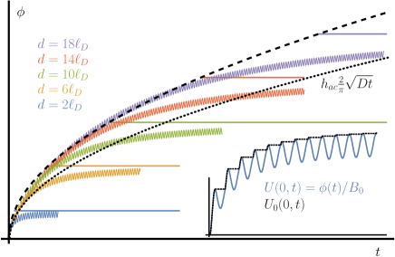
Figure 6: Flux pumping $\phi(t)=B_{0}U(0,t)$ as a function of time. We compare our numerical results (oscillating curves) for different sample sizes $d$ with our analytical model (dotted line), see Eq. (21). A better quantitative agreement with the numerical data is obtained when scaling the analytic result by $1.25$ (dashed line). The horizontal lines indicate for each system the value of the penetrated flux $h_{ac}d/2$ after termination of the initialization process. The inset shows an expanded view at small times of both $U$ and $U_{0}$ at the surface.

Our comparison with recent experiments prozorov_13 refers to a SrPd₂Ge₂ single crystal, a material that is isostructural to the Fe- and Ni-pnictides, of typical size $d\sim 0.5~{}\mathrm{mm}$ in a field $H\sim 0.1~{}\mathrm{T}$ and subject to an $ac$ field $h_{ac}=2~{}\mathrm{\mu T}$ at frequencies $\nu=\omega/2\pi\approx 17~{}\mathrm{MHz}$. With a normal state resistivity sung_11 $\rho_{n}\approx 20~{}\mu\Omega$cm and the upper critical field prozorov_13 $H_{c2}\approx 0.5$ T, we obtain a diffusion length $\ell_{D}\approx 40~{}\mu$m, hence $d/2\ell_{D}\sim 6$. The pinning strength is quantified through the Campbell penetration depth measuring $\lambda_{\rm\scriptscriptstyle C}\approx 10~{}\mu$m, hence $\lambda_{\rm\scriptscriptstyle C}/\ell_{D}\approx 1/4$. The elementary displacement $U(0,\tau)\sim\ell_{d}(h_{ac}/H)$ is of the order of 8 Å at the beginning of the initial diffusion dominated regime and smaller, $U(0,\tau)\sim\lambda_{\rm\scriptscriptstyle C}(h_{ac}/H)\approx 2$ Å in the asymptotic regime, far below the coherence length $\xi\approx 25$ Å. For such a sample and with the above experimental parameters we find that the asymptotic state is reached within about one hundred cycles or $t_{\mathrm{init}}\sim 10~{}\mu\mathrm{s}$, i.e., the transient initialization regime is usually not interfering with the measurement of the Campbell length $\lambda_{\rm\scriptscriptstyle C}$. Each of these cycles typically pumps a fraction of a vortex into the sample, as $(\phi_{0}d)/\Phi_{0}\sim 1/5$. To complete the discussion, we briefly describe the result for the asymptotic regime.

III.2 Asymptotic periodic regime

Once the asymptotic time domain has been reached, vortices exhibit the typical oscillatory behavior near the surface, but with respect to the new critical state that has been shifted upward by $h_{ac}$. Eq. (3) can be solved exactly for a half-infinite space and its solution

$$U(X,t)=U_{0}(X)-\lambda_{\rm\scriptscriptstyle C}(h_{ac}/B_{0})e^{-X/\lambda_{\rm\scriptscriptstyle C}}[1-e^{-i\omega t}]$$ (23)

with the asymptotic max-field,

$$U_{0}(X)=(\phi-h_{ac}X)/B_{0},$$ (24)

and the penetrated $dc$ flux $\phi$ provides a good approximation for a finite-size sample with $d/\lambda_{\mathrm{\scriptscriptstyle C}}\gg 1$. In Eq. (23), the first term $U_{0}$ describes an overall shift of the critical state profile, $\delta B_{0}=-B_{0}\partial_{\scriptscriptstyle X}U_{0}=h_{ac}$, and hence $\phi=h_{ac}d/2$. The second term in Eq. (23) captures the oscillatory and decaying part of the magnetic field $-h_{ac}e^{-X/\lambda_{\rm\scriptscriptstyle C}}[1-e^{-i\omega t}]$. Alternatively, the asymptotic change of the magnetic field profile can be decomposed into an $ac$ component $\delta B_{ac}(X,t)=h_{ac}e^{-X/\lambda_{\rm\scriptscriptstyle C}}e^{-i\omega t}$ and an inhomogeneous $dc$ component $\delta B_{dc}(X)=h_{ac}[1-e^{-X/\lambda_{\rm\scriptscriptstyle C}}]$. The conversion of the $ac$ drive into a $dc$ signal is a unique feature of the critical state and may be observed in an experiment. The Campbell penetration depth $\lambda_{\rm\scriptscriptstyle C}$ is determined by $\alpha_{\mathrm{sp}}$, Eq. (9), involving the jump in force $\Delta f_{\mathrm{pin}}$,

$$\lambda_{\rm\scriptscriptstyle C}^{2}=\frac{B_{0}^{2}}{4\pi\alpha_{\mathrm{sp}}}\sim\frac{\lambda_{\mathrm{\scriptscriptstyle L}}^{2}}{n_{p}a_{0}\xi^{2}\kappa}$$ (25)

with $\kappa$ the Labusch parameter, $\kappa\approx f_{p}a_{0}/\varepsilon_{0}\xi$. Here, $f_{p}$ denotes the pinning force and $\varepsilon_{0}=(\Phi_{0}/4\pi\lambda_{\mathrm{\scriptscriptstyle L}})^{2}$ is the vortex line energy. The small parameter $n_{p}a_{0}\xi^{2}\kappa\ll 1$ defines the three-dimensional strong pinning regime blatter_04 .

The jump in force $\Delta f_{\mathrm{pin}}$ in general depends on the state preparation of the vortex system willa_15b . Hence field-cooled and zero-field cooled vortex states may exhibit different penetration depths and hysteretic effects may show up. This better microscopic understanding of the Campbell penetration depth may then allow to gain more detailed information on the pinscape.

III.3 Non-linear $ac$-response

The above discussion has focused on Campbell penetration, i.e., the linear response regime at small drive $h_{ac}$. As mentioned in the introduction, this has to be distinguished from the Bean penetration at large amplitudes $h_{ac}$. The two regimes are separated by the conditions $\delta j\sim j_{c}$ or $h_{ac}\sim j_{c}\lambda_{\mathrm{\scriptscriptstyle C}}/c$, where the vortex displacement $U\sim(h_{ac}/B_{0})\lambda_{\rm\scriptscriptstyle C}$ matches the pinning length $x_{+}\sim\kappa\xi$ and $\kappa>1$ is the strong pinning parameter labusch_69 . The Bean penetration at large amplitudes exhibits similar behavior on a qualitative level. E.g., using Bean’s original (quasistatic) approach, the $dc$ shift of the critical state profile by $h_{ac}$ occurs during the first (quarter of the) $ac$ cycle; making use of a more sophisticated model with a specific $I$-$V$ characteristics would result in a penetration involving flux-pulses similar to those found above. At large times, after the critical state has been shifted upwards by the $ac$ amplitude $h_{ac}$, the Bean penetration reaches an oscillatory regime where the $ac$ drive generates a simple periodic dynamics on the penetration scale, see Fig. 1 (right panel). On the other hand, the Bean penetration differs from the Campbell penetration on a quantitative level: the penetration depth $\ell_{\mathrm{\scriptscriptstyle B}}\sim ch_{ac}/j_{c}$ within the Bean model scales with $h_{ac}$, resulting in a third harmonic $ac$ magnetic response tinkham_89 . The large displacements (compared to the pinning length $x_{+}$) in the Bean regime do not resolve the internal structure of the pinning centers and hence the $ac$ magnetic response is independent of the state preparation. Finally, the Bean penetration exhibits generic hysteretic properties.

IV Summary and conclusion

Using the results of strong pinning theory, we have studied the complete $ac$ magnetic penetration dynamics in the Campbell regime for a superconducting sample prepared in a critical state. The field penetration proceeds in two phases, a short (on the time scale of the experiment) transient initialization regime where flux enters the sample in a sequence of pulses that shifts the overall critical state by the $ac$ amplitude $h_{ac}$, followed by the standard $ac$ dynamical regime where vortices merely move back and forth in their pinning potentials with no additional net flux entering the sample.

The apparent divergence of the Campbell penetration depth $\lambda_{\rm\scriptscriptstyle C}$ in the phenomenological description prozorov_03 leaves its trace in the pulsed diffusive flux penetration throughout the sample during the initialization regime. After long times, the Campbell length $\lambda_{\mathrm{\scriptscriptstyle C}}$ is a (regular) linear-response parameter containing valuable information on the pinscape that can be extracted from its dependence on the state preparation willa_15b . Despite qualitative similarities between the Campbell (at low $ac$ fields) and the Bean penetration (at higher $ac$ fields) the latter differs by i) its field-dependent penetration depth $\ell_{\mathrm{\scriptscriptstyle B}}\sim ch_{ac}/j_{c}$, ii) the generation of a third harmonics $ac$ signal and iii) the insensitivity to the pinscape structure. Finally, the rectified $dc$ signal $\delta B_{dc}(X)$ induced by the $ac$ (Campbell or Bean) drive is a signature that can be probed in future experimental investigations.

- (1) H. Kamerlingh Onnes, KNAW Proceedings 14 II, 818 (1912).
- (2) W. Meissner and R. Ochsenfeld, Naturwissenschaften 21, 787 (1933).
- (3) F. and H. London, Proc. Roy. Soc. (London) A149, 71 (1935).
- (4) A.A. Abrikosov, Sov. Phys. JETP 5, 1174 (1957).
- (5) L.V. Shubnikov, V.I. Khotkevich, Yu.D. Shepelev, and Yu.N. Riabinin, Zh. Eksp. Teor. Fiz. 7, 221 (1937).
- (6) A.M. Campbell, J. Phys. C 2, 1492 (1969), ibid. 4, 3186 (1971).
- (7) C.P. Bean, Phys. Rev. Lett. 8, 250 (1962).
- (8) R. Prozorov, R.W. Giannetta, N. Kameda, T. Tamegai, J.A. Schlueter, and P. Fournier, Phys. Rev. B 67, 184501 (2003).
- (9) H. Kim, N.H. Sung, B.K. Cho, M.A. Tanatar, and R. Prozorov, Phys. Rev. B 87, 094515 (2013).
- (10) R. Willa, V.B. Geshkenbein, R. Prozorov, and G. Blatter, arXiv:1508.00757 [cond-mat.supr-con] (2015).
- (11) J. Bardeen and M.J. Stephen, Phys. Rev. 140, 1197A (1965).
- (12) R. Labusch, Cryst. Lattice Defects 1, 1 (1969).
- (13) A.I. Larkin and Yu.N. Ovchinnikov, J. Low Temp. Phys. 34, 409 (1979), A.I. Larkin and Yu.N. Ovchinnikov, in Nonequilibrium Superconductivity, edited by D.N. Langenberg and A.I. Larkin (Elsevier, Amsterdam, 1986), p. 493.
- (14) G. Blatter, V.B. Geshkenbein, and J.A.G. Koopmann, Phys. Rev. Lett. 92, 067009 (2004).
- (15) A.E. Koshelev and A.B. Kolton, Phys. Rev. B 84, 104528 (2011).
- (16) A.U. Thomann, V.B. Geshkenbein, and G. Blatter, Phys. Rev. Lett. 108, 217001 (2012).
- (17) At short times the right hand side of expression (20) should be cut off by .
- (18) N.H. Sung, J.-S. Rhyee, and B.K. Cho, Phys. Rev. B 83, 094511 (2011).
- (19) L. Ji, R.H. Sohn, G.C. Spalding, C.J. Lobb, and M. Tinkham, Phys. Rev. B 40, 10936 (1989).