Energy shift due to anisotropic blackbody radiation

Abstract

In many applications a source of the blackbody radiation (BBR) can be highly anisotropic. This leads to the BBR shift that depends on tensor polarizability and on the projection of the total angular momentum of ions and atoms in a trap. We derived a formula for the anisotropic BBR shift and performed numerical calculations of this effect for Ca⁺ and Yb⁺ transitions of experimental interest. These ions were used for a design of high-precision atomic clocks, fundamental physics tests such as the search for the Lorentz invariance violation and space-time variation of the fundamental constants, and quantum information. Anisotropic BBR shift may be one of the major systematic effect in these experiments.

I Introduction

The past five years brought remarkable improvements in both accuracy and stability of atomic clocks  Nicholson et al. (2015); Bloom et al. (2014); Ushijima et al. (2015); Godun et al. (2014); Huntemann et al. (2014). Development of ultra-precise clocks is important for a wide range of applications, including design of absolute gravimeters and gravity gradiometers for geophysical monitoring and research, gravity aided navigation, improved timekeeping and synchronization capabilities, tests of fundamental physics such as Einstein’s theory of relativity, search for variation of fundamental constants through time, space, or coupling to gravitational fields, and exploration of strongly correlated quantum many-body systems Ludlow et al. (2015).

Performing fundamental tests with the atomic clocks and other precision atomic, molecular and optical (AMO) technologies leads to ever increasing requirements for the understanding and control of the systematic errors. Moreover, a number of novel fundamental physics AMO experiments including searches for ultralight (sub-eV) axions, axion-like pseudoscalar and scalar dark matter Van Tilburg et al. (2015); Stadnik and Flambaum (2015); sta and topological defect dark matter Derevianko and Pospelov (2014) have been carried out or proposed, requiring improved understanding of systematic effects in AMO systems.

One of the major experimental and theoretical problems in improving the atomic clock accuracy is a precision determination of atomic clock frequency shift due to blackbody radiation (BBR). In recent experimental works Ushijima et al. (2015); Nicholson et al. (2015) with ⁸⁷Sr optical lattice clocks, the blackbody radiation was identified as the primary source of clock’s uncertainties. A number of measurements and thorough analysis of all systematic effects led to reduction of the Sr clock total uncertainty to the level of $2.1\times 10^{-18}$ in fractional frequency units. However, 65% of the clock uncertainty budget was still due to the BBR shift Nicholson et al. (2015).

A number of other experiments with trapped ions and atoms are sensitive to the BBR effects, including recent tests of local Lorentz invariance (LLI) violation in the electron-photon sector with trapped Ca⁺ Pruttivarasin et al. (2015) ions. Theories aimed at unifying gravity with quantum physics suggest that Nature violates Lorentz symmetry at the Planck scale while suppressing its violation at experimentally achievable energy scales Kostelecký and Potting (1995). The minimal O(1) suppression may lead to Lorentz-violating effects appearing beyond $10^{-17}$ sensitivity level, determined by the ratio of electroweak and Planck scales. Thus, high-precision experiments with atomic systems Hohensee et al. (2013); Pruttivarasin et al. (2015) provide an important route to search for Lorentz violation at low energies. The LLI experiments with trapped ions may be particulary sensitive to anisotropic BBR shift since they are based on monitoring the energy difference between different Zeeman substates as described below. In these experiments, anisotropic BBR shift may become a limiting factor for the ultimate accuracy of the Lorentz violation tests in the electron-photon sector Dzu and this work is strongly motivated by these fundamental studies. BBR effects may also become a source of decoherence in larger-scale quantum information experiments with trapped ions due to a change in the environmental temperature or temperature gradients during the computation.

Calculations of blackbody radiation shifts are usually done assuming that the BBR radiation is isotropic.

A detailed consideration of the isotropic BBR effect in conventional electric dipole approximation was carried out in Farley and Wing (1981). Multipolar theory of isotropic BBR shift of atomic energy levels (as well as its implications for optical lattice clocks) was developed in Porsev and Derevianko (2006). However, in practice the source of BBR can be highly anisotropic and even may have a small angular size. As a result, a lot of experimental efforts is required to make the BBR field uniform and with a known temperature Nicholson et al. (2015); Ushijima et al. (2015); Beloy et al. (2014). For this reason a proper calculation of the anisotropic BBR shift is necessary. Also, this effect can be of interest by itself as a physical phenomenon. We note that the problem of anisotropic BBR effect, discussed in the present work, does not arise in experiments with alkaline-earth atoms aiming to create an atomic clock in the ${}^{1}\!S_{0}-\,^{3}\!P^{o}_{0}$ transition because the states with total angular momenta $J=0$ are involved.

II General formalism

The isotropic BBR shift of an energy level is proportional to scalar static polarizability of this level Farley and Wing (1981); Porsev and Derevianko (2006). In the case of anisotropic blackbody radiation, an additional contribution that depends on the projection of a thermal photon wave vector $\boldsymbol{k}$ to the $z$ axis arises. We show below that it is determined by the tensor polarizability of the level. This contribution is particularly important when we consider BBR frequency shift of a $|JM\rangle$ - $|JM^{\prime}\rangle$ transition, where $M$ and $M^{\prime}$ are the projections of the total angular momentum ${\bf J}$ to the $z$ axis, and we assume $J$ and $M$ to be good quantum numbers for the atomic states. The scalar polarizabilities of the Zeeman substates $|JM\rangle$ and $|JM^{\prime}\rangle$ are practically identical differing only due to a very small difference in the energy denominators. As a result, the isotropic BBR frequency shift is completely negligible in this case. In contrast, the anisotropic BBR shift of the energy level depends on $M^{2}$ and can be noticeably different for the different $M$ substates. The same issue arises for the hyperfine states with different $M_{F}$.

Such a systematic effect arose in a recent record-high precision experiment aimed at the search for local Lorentz invariance violation in the electron-photon sectors using a superposition of two Ca⁺ ions Pruttivarasin et al. (2015). In the experiment, the energy difference between the $M=1/2$ and 5/2 substates of the $3d~{}^{2}\!D_{5/2}$ multiplet, monitored over 23 h served as a probe of Lorentz-violating effects.

The anisotropic BBR shift produces a differential shift between $M=1/2$ and 5/2 states mimicking the Lorentz-violating effects. Thus, anisotropic BBR is an important systematic effect. It was demonstrated in Dzu that a factor of $10^{5}$ higher sensitivity to Lorentz violation may be achieved with a similar experimental scheme with Yb⁺ by monitoring the ($4f^{13}\,6s^{2}$) ${}^{2}\!F_{7/2,M=7/2}-\,^{2}\!F_{7/2,M=1/2}$ frequency difference. Since this experiment will probe LLI at much higher sensitivity, study of anisotropic BBR is needed as it can be a major systematic effect for such an experiment.

We note that singly ionized ytterbium ¹⁷¹Yb⁺ with ultranarrow optical ${}^{2}\!S_{1/2}$ - ${}^{2}\!D_{3/2}$ and ${}^{2}\!S_{1/2}$ - ${}^{2}\!F_{7/2}$ transitions is also being pursued for a realization of an optical atomic clock and search for the temporal variation of the fine-structure constant $\alpha$ and the proton-to-electron mass ratio $m_{p}/m_{e}$ Godun et al. (2014); Huntemann et al. (2014).

The problem of anisotropic BBR shift of energy levels is practically unexplored so far, but may cause systematic effects in a variety of experiments. In this work, we derived a general formula for the BBR shift of an energy level produced by a point-like source. A generalization to a finite source is obtained by integration over angles of emitted thermal photons. The result is expressed in terms of the scalar and tensor polarizabilities of the atomic level. We also performed numeric calculation of the BBR frequency shifts for the Ca⁺ ${}^{2}\!D_{5/2,M=5/2}$ - ${}^{2}\!D_{5/2,M=1/2}$ transition and Yb⁺ ${}^{2}\!F_{7/2,M=7/2}$ - ${}^{2}\!F_{7/2,M=1/2}$ transitions due to their relevance to searches for Lorentz violation.

An interaction of an atom in the state $|0\rangle$ with the electric field of a thermal photon emitted to a solid angle $d\Omega$ leads to a blackbody radiation shift of an energy level. After integration over photon frequency, the BBR shift of the energy level $|0\rangle$ can be written as

$$\frac{dE}{d\Omega}=A\sum_{\epsilon}\sum_{i,k=1}^{3}\alpha_{ik}\epsilon_{i}\epsilon_{k}^{\ast}.$$ (1)

Here, we use a three-dimensional transverse gauge for photon polarization $\epsilon_{\mu}=(0,\boldsymbol{\epsilon})$ with polarization $\boldsymbol{\epsilon}$ normalized to the unit. Since photons are transverse, in this gauge $\boldsymbol{k\epsilon}=0$. The elements of the symmetric tensor $\alpha_{ik}$ are defined as

$$\alpha_{ik}=2\sum_{m}\frac{\langle 0|d_{i}|m\rangle\langle m|d_{k}|0\rangle}{\omega_{m0}},$$ (2)

where $\mathbf{d}=-\mathbf{r}$ is the electric dipole moment operator and $\omega_{m0}\equiv E_{m}-E_{0}$ is the difference between energy levels of the intermediate and $|0\rangle$ states. We use atomic units, i.e., $|e|=\hbar=m_{e}=1$. An explicit form of the factor $A$ is not important for the following derivation and we will restore it later.

In the following we discuss only BBR effect caused by the electric field. The BBR caused by a magnetic field was considered in Ref. Itano et al. (1982) for a number of monovalent ions and proved to be negligible. Using the multipolar theory of blackbody radiation, developed in Porsev and Derevianko (2006), one can show that for the transitions in the Ca⁺ and Yb⁺ ions, which will be discussed below, this effect can also be neglected.

The electric dipole static polarizability of an atom in the state $|0\rangle$ is defined as

$${\alpha_{\rm pol}}\equiv\alpha_{zz}=2\sum_{m}\frac{|\langle 0|d_{z}|m\rangle|^{2}}{\omega_{m0}}.$$ (3)

It can be conveniently decomposed into scalar and tensor parts: ${\alpha_{\rm pol}}=\alpha_{s}+\alpha_{t}$ with the scalar polarizability $\alpha_{s}$ given by

$$\alpha_{s}=\frac{1}{3}\sum_{i}\alpha_{ii}=\frac{2}{3}\sum_{m}\frac{|\langle 0|\mathbf{d}|m\rangle|^{2}}{\omega_{m0}}.$$ (4)

The summation over photon polarizations in Eq. (1) is carried out using

$$\sum_{\epsilon}{\epsilon_{i}\epsilon_{k}^{*}}=\delta_{ik}-n_{i}n_{k},$$

where $\boldsymbol{n}\equiv\boldsymbol{k}/k$. Then, Eq. (1) is reduced to

$$\frac{dE}{d\Omega} = A\left[\sum_{i}\alpha_{ii}-\sum_{i,k}\alpha_{ik}n_{i}n_{k}\right].$$

$$= A\left[3\alpha_{s}-\sum_{i,k}\alpha_{ik}n_{i}n_{k}\right].$$

The BBR shift in our case depends on the angle $\theta$ between the direction of the photon momentum $\boldsymbol{k}$ and the quantization axis $z$, defined by the direction of the magnetic field. It is convenient to choose the vector $\boldsymbol{k}$ in the $xz$ plane, i.e., $k_{y}=0$. Taking into account Eq. (4) and noting that the product of the matrix elements $\langle 0|d_{x}|n\rangle\langle n|d_{z}|0\rangle=0$ and, respectively, $\alpha_{zx}=\alpha_{xz}=0$, we obtain

$$\frac{dE}{d\Omega} = A\left[3\alpha_{s}-\alpha_{xx}n_{x}^{2}-\alpha_{zz}n_{z}^{2}\right]$$

$$= A\left[3\alpha_{s}-\alpha_{xx}\sin^{2}\theta-\alpha_{zz}\cos^{2}\theta\right].$$

Accounting for the fact that $\alpha_{xx}=\alpha_{yy}$ and, hence,

$$\alpha_{xx}=\frac{3\alpha_{s}-\alpha_{zz}}{2},$$ (5)

we express $dE/d\Omega$ through $\alpha_{s}$, $\alpha_{t}$, and $\cos^{2}\!\theta$. After simple transformations we arrive at

$$\frac{dE}{d\Omega}=A^{\prime}\left[\alpha_{s}+\frac{1-3\cos^{2}\!\theta}{4}\alpha_{t}\right],$$ (6)

where $A^{\prime}=2A$. The factor $A^{\prime}$ can be easily determined, if we note that after integrating over $d\Omega={\rm sin}\theta\,d\theta\,d\phi$ the second term in Eq. (6) disappears and we obtain $\Delta E=4\pi A^{\prime}\alpha_{s}$. On the other hand, we have to arrive at the standard formula for isotropic BBR shift which, neglecting dynamic corrections, is given by Porsev and Derevianko (2006)

$$\Delta E=-\frac{2}{15}(\alpha\pi)^{3}T^{4}\alpha_{s},$$

where the temperature $T$ is given in a.u.. Finally, we obtain

$$dE=-\frac{2}{15}(\alpha\pi)^{3}T^{4}$$

$$\times\left[\alpha_{s}+\frac{1-3\cos^{2}\!\theta}{4}\,\frac{3M^{2}-J(J+1)}{J(2J-1)}\alpha_{2}\right]\frac{d\Omega}{4\pi}.$$ (7)

Here we represent the tensor part $\alpha_{t}$ by

$$\alpha_{t}=\frac{3M^{2}-J(J+1)}{J(2J-1)}\alpha_{2},$$ (8)

where $\alpha_{2}$ is the tensor polarizability of the state $|0\rangle$.

It may be instructive to present a different derivation of Eq. (6), starting again from Eq. (1). Assuming the polarization vectors $\epsilon_{1,2}$ to be real we can write

$$\frac{dE}{d\Omega}=A\sum_{i=1}^{2}\left(\alpha_{xx}\epsilon_{ix}^{2}+\alpha_{yy}\epsilon_{iy}^{2}+\alpha_{zz}\epsilon_{iz}^{2}\right).$$ (9)

Taking into account that $\alpha_{xx}=\alpha_{yy}$ and using the normalization condition $\epsilon_{ix}^{2}+\epsilon_{iy}^{2}+\epsilon_{iz}^{2}=1$ and Eq. (5), after simple transformations, we obtain

$$\frac{dE}{d\Omega}=A\sum_{i=1}^{2}\left(\alpha_{s}+\frac{3\,{\rm cos}^{2}\theta_{i}-1}{2}\alpha_{t}\right),$$ (10)

where $\theta_{i}$ is the angle between the photon polarization vector $\boldsymbol{\epsilon}_{i}$ and the $z$ axis.

Summing up over index $i$ in Eq. (10), and using condition

$${\rm cos}^{2}\theta_{1}+{\rm cos}^{2}\theta_{2}+{\rm cos}^{2}\theta=1,$$ (11)

which is valid because the vectors $\boldsymbol{\epsilon}_{1}$, $\boldsymbol{\epsilon}_{2}$, and $\boldsymbol{k}$ are mutually orthogonal, we arrive at Eq. (6).

III Anisotropic BBR shift for ${}^{2S+1}\!L_{J,M}-\,^{2S+1}\!L_{J,M^{\prime}}$ transitions

We now apply Eq. (7) to the case of a $|JM\rangle-|JM^{\prime}\rangle$ transition between the ionic or atomic Zeeman sublevels. As we discussed above, the isotropic BBR shift, proportional to the scalar part of the polarizability, is very small for such a transition because it results only from a small difference between $|JM\rangle$ and $|JM^{\prime}\rangle$ energy levels. The main effect comes from the tensor part of the polarizability.

Using Eqs. (7) and (8) we write the $|JM\rangle-|JM^{\prime}\rangle$ transition frequency BBR shift $dE_{\rm t}$ as

$$dE_{\rm t} \equiv dE_{JM}-dE_{JM^{\prime}}$$ (12)

$$\approx \frac{(\alpha\pi)^{3}T^{4}}{10}(3\cos^{2}\!\theta-1)\,\frac{M^{2}-{M^{\prime}}^{2}}{J(2J-1)}\,\alpha_{2}\,\frac{d\Omega}{4\pi}.$$

Integration of Eq. (12) over fixed solid angle $\Omega_{1}$ leads to the BBR shift, corresponding to a maximal anisotropy 100%, when the BBR is emitted to this solid angle and there is no BBR from the remainder.

Let us consider a more realistic case when a certain portion of photons is emitted to the solid angle $\Omega_{1}$ at the temperature $T_{1}$ and another portion of photons is emitted to the solid angle $\Omega_{2}$ at the temperature $T_{2}$, so that $\Omega_{1}+\Omega_{2}=4\pi$. The corresponding differential BBR shifts, which we designate as $dE^{(k)}_{\rm t}$ ($k=1,2$), are given by Eq. (12) with $T=T_{k}$.

Then, the total BBR shift can be found as

$$\Delta E_{\rm t} = \left[\int_{0}^{\Omega_{1}}\frac{dE^{(1)}_{\rm t}}{d\Omega}+\int_{\Omega_{1}}^{4\pi}\frac{dE^{(2)}_{\rm t}}{d\Omega}\right]d\Omega$$ (13)

$$= \int_{0}^{\Omega_{1}}\left[\frac{dE^{(1)}_{\rm t}}{d\Omega}-\frac{dE^{(2)}_{\rm t}}{d\Omega}\right]d\Omega.$$

Performing integration in Eq. (13) over azimuthal angle $\varphi$ from zero to $2\pi$ and over $\theta$ from zero to a fixed value $\theta_{1}$, we obtain

$$\Delta E_{\rm t} \approx \frac{(\alpha\pi)^{3}(T_{1}^{4}-T_{2}^{4})}{20}\,\frac{M^{2}-{M^{\prime}}^{2}}{J(2J-1)}\,\alpha_{2}$$ (14)

$$\times \cos\theta_{1}(1-\cos^{2}\!\theta_{1}).$$

As seen from Eq. (14), $\Delta E_{\rm t}$ turns to zero if $T_{1}=T_{2}$, as it should be because it corresponds to the isotropic BBR case.

It follows from Eq. (14) that the BBR shift is $\sim\theta_{1}^{2}$ when $\theta_{1}$ is small. Thus, this shift is greatly reduced with decrease in the solid angle to which the thermal photons are emitted. On the other hand, the anisotropic BBR shift is equal to zero when $\theta_{1}=90^{\circ}$. When $\theta_{1}$ changes from 30 to $60^{\circ}$, $\cos\theta_{1}(1-\cos^{2}\!\theta_{1})$ changes from 0.22 to 0.38.

Below we consider the anisotropic BBR shifts for the ${}^{2}\!D_{5/2,M=5/2}$ - ${}^{2}\!D_{5/2,M=1/2}$ transition in Ca⁺ and for the ${}^{2}\!F_{7/2,M=7/2}$ - ${}^{2}\!F_{7/2,M=1/2}$ transition in Yb⁺.

III.1 Anisotropic BBR shift for the ${}^{2}\!D_{5/2,M=5/2}-\,^{2}\!D_{5/2,M=1/2}$ transition in Ca⁺.

In a recent paper Pruttivarasin et al. (2015), the ${}^{2}\!D_{5/2,M=5/2}$ - ${}^{2}\!D_{5/2,M=1/2}$ transition in Ca⁺ was used to search for Lorentz invariance violation at a level comparable to the ratio between the electroweak and Planck energy scales.

Using Eq. (14), we estimate the anisotropic BBR shift for this transition. The most accurate value of the tensor polarizability for the ${}^{2}\!D_{5/2}$ state was obtained in Ref. Safronova and Safronova (2011), $\alpha_{2}=-24.51(29)$ a.u.. To illustrate dependence of the BBR shift from the temperatures $T_{1}$ and $T_{2}$, we find $\Delta E_{\rm t}$ for three values of $T_{1}$ (500, 420, and 350 K) and $T_{2}$ = 300 K. Substituting these values in Eq. (14), taking into account that for the room temperature 300 K $(\alpha\pi)^{3}T^{4}/20\approx 4.9069\times 10^{-19}$ a.u., and expressing final results in Hz, we obtain

$$\Delta E_{\rm t} \approx \cos\theta_{1}(1-\cos^{2}\!\theta_{1})$$ (18)

$$\times \left\{\begin{array}[]{l}-0.319\,\text{(Hz)},\,T_{1}=500\,{\rm K},\\ -0.135\,\text{(Hz)},\,T_{1}=420\,{\rm K},\\ -0.040\,\text{(Hz)},\,T_{1}=350\,{\rm K}.\end{array}\right.$$

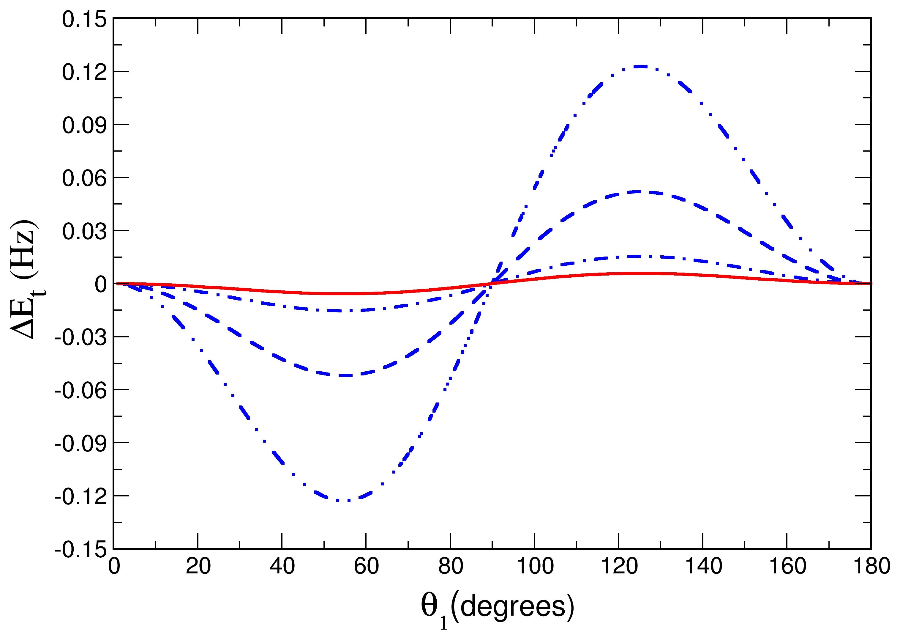
Figure 1: (Color online) Dependence of $\Delta E_{\rm t}$ from the angle $\theta_{1}$ for Ca⁺ (see Eq. (18)) is represented by (blue) dash-dot-dotted line for $T_{1}$ = 500 K, by dashed line for $T_{1}$ = 420 K, and by dot-dashed line for $T_{1}$ = 350 K. Dependence of $\Delta E_{\rm t}$ from $\theta_{1}$ for Yb⁺ (see Eq. (25)) is represented by (red) solid line for $T_{1}$ = 450 K. The temperature $T_{2}$ = 300 K in all cases.

These dependences of $\Delta E_{\rm t}$ from the angle $\theta_{1}$ in Ca⁺ ${}^{2}\!D_{5/2,M=5/2}$ - ${}^{2}\!D_{5/2,M=1/2}$ transition are illustrated in Fig. 1 by three (blue) lines. As expected, $\Delta E_{\rm t}$ is equal to zero at $\theta_{1}=0$ and $180^{\circ}$. The angle $\theta_{1}=180^{\circ}$ corresponds to isotropic radiation. $\Delta E_{\rm t}$ also crosses zero when $\theta_{1}$ is $90^{\circ}$. This case corresponds to isotropic radiation in the upper hemisphere. The energy shifts due to the BBR effect are largest for $\theta_{1}\approx 55^{\circ}$.

III.2 Anisotropic BBR shift for the ${}^{2}\!F_{7/2,M=7/2}-\,^{2}\!F_{7/2,M=1/2}$ transition in Yb⁺.

Recent work  Dzu identified several factors affecting the precision of the local Lorentz invariance tests with trapped ions. The two most important factors are the lifetime of the excited atomic state used in the Lorentz invariance probe and sensitivity of this state to the Lorentz invariance violation effect, i.e., the size of the matrix element of the corresponding operator. Both features are supplied by the metastable $4f^{13}6s^{2}\,{}^{2}\!F_{7/2}$ state of the Yb⁺ ion, and the ${}^{2}\!F_{7/2,M=7/2}$ - ${}^{2}\!F_{7/2,M=1/2}$ transition was proposed as the probe of Lorentz-violating effects. To estimate this BBR shift we need to evaluate the value of the tensor polarizability $\alpha_{2}(^{2}\!F_{7/2})$. We carried out calculations in the framework of 15-electron configuration interaction (CI) method, following the approach described in Ref. Porsev et al. (2012).

The main features of this approach are briefly described below. All electrons are divided into the core and valence electrons. In our case [$1s^{2}$,…,$5p^{6}$] are the core electrons while 15 outer electrons belong to the valence subspace.

In the framework of the CI method we solve the eigenvalue problem

$$H_{\rm CI}\Phi=E_{\rm CI}\Phi,$$ (19)

where the many-electron wave functions $\Phi$ belong to the valence subspace and are presented as a linear combination of Slater determinants,

$$\Phi=\sum_{{\rm det}_{I}}C_{I}|{\rm det}_{I}\rangle.$$ (20)

The CI Hamiltonian can be written as

$$H_{\rm CI}=E_{\rm core}+\sum_{i>N_{\rm core}}{h^{\rm CI}_{i}}+\sum_{j>i>N_{\rm core}}V_{ij}\,,$$ (21)

where $N_{\rm core}$ is the number of core electrons, $E_{\rm core}$ is the energy of the core which includes kinetic energy of the core electrons, Coulomb energy of their interaction with the nucleus and potential energy of the core-core electrostatic interaction. The core-valence interaction, kinetic energy of the valence electrons and their interaction with the nucleus are included in the one-electron operators $h^{\rm CI}_{i}$. The last term in Eq. (21) accounts for the interaction between valence electrons.

We start from solving the Dirac-Fock equations for the [$1s^{2}$,…,$4f^{13}6s^{2}$] configuration. Then the $6p_{j}$ and $5d_{j}$ orbitals are constructed for the $4f^{13}6s6p$ and $4f^{13}6p5d$ configurations, correspondingly. The basis set used in the CI calculations included also virtual orbitals up to $8s$, $8p$, $7d$, $7f$, and $5g$. We form configuration space by allowing single and double excitations for the odd-parity states from the $4f^{14}6p$, $4f^{13}6s^{2}$ and $4f^{13}5d6s$ configurations and for the even-parity states from the $4f^{14}6s$, $4f^{13}6s6p$ and $4f^{13}6p5d$ configurations to the orbitals of the basis set listed above.

Solving the relativistic multiparticle Schrödinger equation, Eq. (19) gives the eigenvector of the $4f^{13}6s^{2}$ ${}^{2}\!F_{7/2}$ state which we use to determine the tensor polarizability of this state.

Using formalism of the reduced matrix elements we can write the expression for the tensor polarizability of the state $\Phi_{0}$ with total angular momentum $J$ as Kozlov and Porsev (1999)

$$\alpha_{2}=4\left(\frac{5J(2J-1)}{6(2J+3)(2J+1)(J+1)}\right)^{1/2}$$ (24)

$$\times \sum_{n}(-1)^{J+J_{n}}\left\{\begin{array}[]{ccc}J&1&J_{n}\\ 1&J&2\end{array}\right\}\frac{|\langle\Phi_{0}||d||\Phi_{n}\rangle|^{2}}{E_{n}-E_{a}},$$

where $J_{n}$ is the total angular momentum of the intermediate state $\Phi_{n}$.

A direct summation over all intermediate states in Eq. (24) requires a knowledge of the complete set of eigenstates of the Hamiltonian (19). Practically, this is impossible when dimension of a CI space exceeds few thousand determinants, as in our case. To find the electric dipole tensor polarizability of the $4f^{13}6s^{2}$ ${}^{2}\!F_{7/2}$ state we use the method of solution of an inhomogeneous equation, described in detail in Kozlov and Porsev (1999). The random-phase-approximation corrections are also included.

The result of our computation of the tensor polarizability is $\alpha_{2}(^{2}\!F_{7/2})\approx-2$ a.u.. Using this value and $T_{1}$ = 450 K and $T_{2}$ = 300 K, we obtain from Eq. (14)

$$\Delta E_{\rm t} \approx -0.015\,\cos\theta_{1}(1-\cos^{2}\!\theta_{1})\,\,{\rm Hz}.$$ (25)

The dependence of $\Delta E_{\rm t}$ on the angle $\theta_{1}$ is shown in Fig. 1 by a (red) solid line. While the general behavior of $\Delta E_{\rm t}$ for Yb⁺ is the same at $\theta_{1}$ = 0, 90, and $180^{\circ}$ as in Ca⁺, the $\Delta E_{\rm t}$ is much smaller in the Yb⁺ transition considered here than in the Ca⁺ one. Suppression of the anisotropic blackbody radiation in the ${}^{2}\!F_{7/2,M=7/2}$ - ${}^{2}\!F_{7/2,M=1/2}$ Yb⁺ transition is due to compactness of the Yb⁺ $4f$ orbital, resulting in the value of tensor polarizability, which is an order of magnitude smaller than that for the ${}^{2}\!D_{5/2}$ state of Ca⁺. Therefore, the anisotropic BBR shift is strongly suppressed for transition between substates of the Yb⁺ ${}^{2}F_{7/2}$ multiplet, and for $T_{1}$ = 450 and $T_{2}$ = 300 K its maximal (absolute) value at $\theta_{1}\approx 55^{\circ}$ is equal to 5.8 mHz.

To conclude, we derived the formula for the anisotropic BBR shift of an energy level and performed numerical calculations of this effect for Ca⁺ and Yb⁺ transitions of interest for study of Lorentz violation. We demonstrated that this effect strongly depends on the magnitude of the tensor polarizability of the level. In high-precision experiments, the anisotropic BBR can be a major systematic effect that should be specifically addressed in determining experimental uncertainties.

M.S.S. thanks the School of Physics at University of New South Wales (UNSW), Sydney, Australia for hospitality and acknowledges support from the Gordon Godfrey Fellowship program, UNSW. This work was supported by NSF Grants No. PHY-1404156, No. PHY-1212442, and No. PHY-1520993 and the Australian Research Council.

References

- Nicholson et al. (2015) T. L. Nicholson, S. L. Campbell, R. B. Hutson, G. E. Marti, B. J. Bloom, R. L. McNally, W. Zhang, M. D. Barrett, M. S. Safronova, G. F. Strouse, et al., Nature Comm. 6, 6896 (2015).
- Bloom et al. (2014) B. J. Bloom, T. L. Nicholson, J. R. Williams, S. L. Campbell, M. Bishof, X. Zhang, W. Zhang, S. L. Bromley, and J. Ye, Nature 506, 71 (2014).
- Ushijima et al. (2015) I. Ushijima, M. Takamoto, M. Das, T. Ohkubo, and H. Katori, Nat. Photonics 9, 185 (2015).
- Godun et al. (2014) R. M. Godun, P. B. R. Nisbet-Jones, J. M. Jones, S. A. King, L. A. M. Johnson, H. S. Margolis, K. Szymaniec, S. N. Lea, K. Bongs, and P. Gill, Phys. Rev. Lett. 113, 210801 (2014).
- Huntemann et al. (2014) N. Huntemann, B. Lipphardt, C. Tamm, V. Gerginov, S. Weyers, and E. Peik, Phys. Rev. Lett. 113, 210802 (2014).
- Ludlow et al. (2015) A. D. Ludlow, M. M. Boyd, J. Ye, E. Peik, and P. O. Schmidt, Rev. Mod. Phys. 87, 637 (2015).
- Van Tilburg et al. (2015) K. Van Tilburg, N. Leefer, L. Bougas, and D. Budker, Phys. Rev. Lett. 115, 011802 (2015).
- Stadnik and Flambaum (2015) Y. V. Stadnik and V. V. Flambaum, Phys. Rev. Lett. 115, 201301 (2015).
- (9) Y. V. Stadnik and V. V. Flambaum, arXiv:1504.01798.
- Derevianko and Pospelov (2014) A. Derevianko and M. Pospelov, Nature Physics 10, 933 (2014).
- Pruttivarasin et al. (2015) T. Pruttivarasin, M. Ramm, S. G. Porsev, I. Tupitsyn, M. S. Safronova, M. A. Hohensee, and H. Häffner, Nature 517, 592 (2015).
- Kostelecký and Potting (1995) V. A. Kostelecký and R. Potting, Phys. Rev. D 51, 3923 (1995).
- Hohensee et al. (2013) M. A. Hohensee, N. Leefer, D. Budker, C. Harabati, V. A. Dzuba, and V. V. Flambaum, Phys. Rev. Lett. 111, 050401 (2013).
- (14) V. A. Dzuba, V. V. Flambaum, M. S. Safronova, S. G. Porsev, T. Pruttivarasin, M. A. Hohensee, and H. Häffner, Nat. Phys. (2016), doi: 10.1038/nphys3610; arXiv:1507.06048.
- Farley and Wing (1981) J. W. Farley and W. H. Wing, Phys. Rev. A 23, 2397 (1981).
- Porsev and Derevianko (2006) S. G. Porsev and A. Derevianko, Phys. Rev. A 74, 020502(R) (2006).
- Beloy et al. (2014) K. Beloy, N. Hinkley, N. B. Phillips, J. A. Sherman, M. Schioppo, J. Lehman, A. Feldman, L. M. Hanssen, C. W. Oates, and A. D. Ludlow, Phys. Rev. Lett. 113, 260801 (2014).
- Itano et al. (1982) W. M. Itano, L. L. Lewis, and D. J. Wineland, Phys. Rev. A 25, 1233 (1982).
- Safronova and Safronova (2011) M. S. Safronova and U. I. Safronova, Phys. Rev. A 83, 012503 (2011).
- Porsev et al. (2012) S. G. Porsev, M. S. Safronova, and M. G. Kozlov, Phys. Rev. A 86, 022504 (2012).
- Kozlov and Porsev (1999) M. G. Kozlov and S. G. Porsev, Eur. Phys. J. D 5, 59 (1999).