Detector resolution correction for width of intermediate states in three particle decays

Abstract

We propose a method that allows to take into account detector resolution in the partial wave analysis event-by-event fit as a special case. Implementation of the method is discussed and the applicability of the method is studied for the $J/\psi\to K^{*\pm}K^{\mp}\to K^{+}K^{-}\pi^{0}$ and $J/\psi\to K_{2}(1430)^{\pm}K^{\mp}\to K^{+}K^{-}\pi^{0}$ decays.

1 Introduction

The most of partial wave analyses (PWA) are performed in the framework of the maximum likelihood method. For a typical set-up the log-likelihood function is $s=-\sum_{i}\ln P_{i}$, where $i$ runs over selected data events and $P_{i}$ is the probability to observe an event with measured momenta of final particles $p_{i}$. The latter is given by $P_{i}=\epsilon_{i}\sigma_{i}/\int(\epsilon\sigma)d\Phi$, where $\epsilon_{i}$ is the selection efficiency for the kinematics of event $i$, $\sigma_{i}=\sigma(p_{i})$ is the differential cross section (depending on the fitted parameters) and the integral gives the overall normalization factor. To take into account the detector resolution one has to introduce a convolution with detector response function: $\epsilon\sigma\to R\otimes(\epsilon\sigma)$. In general case such convolution can not be performed within reasonable CPU time. Here we show that for a special case discussed below the detector resolution can be taken into account.

Without loss of generality the method will be described in application to the $J/\psi\to K^{*\pm}K^{\mp}\to K^{+}K^{-}\pi^{0}$ decay, where we are interested in measuring the width of $K^{*}$ and assume that $J/\psi$ is produced in a $e^{+}e^{-}$ collider experiment. We also apply the method to $J/\psi\to K_{2}(1430)^{\pm}K^{\mp}\to K^{+}K^{-}\pi^{0}$.

2 Method

Typically the cross section is calculated from measured momenta of final state particles. For the following we consider the case when these momenta are taken after the kinematic fit, so that the total four-momentum is known precisely and is not smeared.

The method is based on three main assumptions:

• We assume that the kinematical variables the cross section depends on can be divided into two groups such that in the calculation of the convolution of cross section with the detector response function, the cross section dependence on the second group of variables can be neglected. The qualitative definition will be given later.

• The mass resolution in the studied kinematic channel is much smaller than the width of the studied resonance (in our example $\sigma_{K\pi}\ll\Gamma_{K^{*}}$, where $\sigma_{K\pi}$ stands for the mass resolution in the $K\pi$ channel).

• Monte-Carlo simulation of detector resolution and efficiency is consistent with real data processing.

From general arguments the differential cross section of the $J/\psi\to K^{+}K^{-}\pi^{0}$ decay in the center-of-mass reference frame depends on four variables ($J/\psi$ in relativistic $e^{+}e^{-}$ collisions is produced with $J_{z}=\pm 1$, so we measure $3\times 3$ particle momenta with overall 4-momentum constraint and rotation symmetry along the beam axis) denoted by $a_{k}$, $k=1..4$. The Breit-Wigner parts of the amplitude depend on invariant masses of any two pairs of final particles (the invariant mass of the third pair depends on the first two), for computation convenience we took $M^{2}(K^{+}\pi^{0})$ and $M^{2}(K^{-}\pi^{0})$. The other two variables are arguments of the angular parts of the amplitude and we do not specify them.

For an event with the measured momenta $q$, the convolution reads:

$$\begin{split}(R\otimes\sigma\epsilon)(q)&=\int R(q^{\prime}-q,q)\epsilon(q^{\prime})\sigma(a(q^{\prime}))dq^{\prime}\approx\\ &\approx\epsilon(q)\int R(q^{\prime}-q,q)\sigma(a(q^{\prime}))dq^{\prime},\\ \end{split}$$

where $R(q^{\prime}-q,q)$ is the detector response function (note, due to the kinematic fit not all momenta here are independent and that is taken into account in $R(q^{\prime}-q,q)$). For the following we will not need the explicit form of $R(q^{\prime}-q,q)$. Then we take integrals and change variables to $a$:

$$\begin{split}\int R(q^{\prime}-q,q)\sigma(a(q^{\prime}))dq^{\prime}=\int\tilde{R}(a^{\prime}-a^{q},q)\sigma(a^{\prime})da^{\prime}=\\ =\int\tilde{R}(\delta a,q)\biggl{(}\sigma(a^{q})+\sum_{k}\frac{\partial\sigma(a)}{\partial a_{k}}\delta a_{k}+\sum_{k,l}\frac{1}{2}\frac{\partial^{2}\sigma(a)}{\partial a_{k}\partial a_{l}}\delta a_{k}\delta a_{l}+\\ +O(\delta a^{3})\biggr{)}d\delta a=\sigma\Big{|}_{a^{q}}+\sum_{k}\frac{\partial\sigma}{\partial a_{k}}\Big{|}_{a^{q}}\cdot\langle\delta a_{k}\rangle+\\ +\sum_{k,l}\frac{1}{2}\frac{\partial^{2}\sigma}{\partial a_{k}\partial a_{l}}\Big{|}_{a^{q}}\cdot\langle\delta a_{k}\delta a_{l}\rangle+\int\tilde{R}(\delta a,q)O(\delta a^{3})d\delta a.\end{split}$$ (1)

Here averages $\langle\delta a_{k}\rangle$ and $\langle\delta a_{k}\delta a_{l}\rangle$ are calculated using $\tilde{R}(\delta a,q)$ as weight. The last step is to take into account in equation 1 only variables that cross section strongly depends on. Quantitatively we assume that

$$\begin{split}\sum_{\alpha}\frac{\partial\sigma}{\partial a_{\alpha}}\Big{|}_{a^{q}}\cdot\langle\delta a_{\alpha}\rangle+\sum_{\alpha,\beta}\frac{1}{2}\frac{\partial^{2}\sigma}{\partial a_{\alpha}\partial a_{\beta}}\Big{|}_{a^{q}}\cdot\langle\delta a_{\alpha}\delta a_{\beta}\rangle\gg\\ \sum_{\zeta}\frac{\partial\sigma}{\partial a_{\zeta}}\Big{|}_{a^{q}}\cdot\langle\delta a_{\zeta}\rangle+\sum_{\zeta\xi}\frac{1}{2}\frac{\partial^{2}\sigma}{\partial a_{\zeta}\partial a_{\xi}}\Big{|}_{a^{q}}\cdot\langle\delta a_{\zeta}\delta a_{\xi}\rangle,\end{split}$$

where indexes $\alpha$ and $\beta$ run over the first group of variables ($M^{2}(K^{+}\pi^{0})$ and $M^{2}(K^{-}\pi^{0})$), $\zeta$ and $\xi$ run over the second group. Finally one gets the computation formula:

$$\begin{split}(R\otimes\sigma)(q)\approx\\ \sigma(q)+\sum_{\alpha}\frac{\partial\sigma}{\partial M^{2}_{\alpha}}\Big{|}_{(q)}\langle\delta M^{2}_{\alpha}\rangle+\sum_{\alpha,\beta}\frac{1}{2}\frac{\partial^{2}\sigma}{\partial M^{2}_{\alpha}\partial M^{2}_{\beta}}\Big{|}_{(q)}\langle\delta M^{2}_{\alpha}\delta M^{2}_{\beta}\rangle.\end{split}$$ (2)

Derivatives and averages are calculated numerically, the averages can be taken as constants in the fit. Despite of the chosen variables, this expression can be also used for resonances in the $K^{+}K^{-}$ channel.

3 Notes on implementation

The decay amplitude in a particular kinematic channel is a product of angular and Breit-Wigner-like parts. So, calculating cross section derivatives in the given approximation, one can vary only invariant mass squared keeping the angular part constant, which can be easily implemented in the existing PWA code. For our tests the first and the second cross section derivatives were calculated in the simplest finite-difference scheme (it required calculation of the Breit-Wigner amplitude part in six additional points).

As resolution is much smaller than the width of the studied intermediate resonance the fit can be done iteratively: the first fit is performed ignoring detector resolution effects, averages in equation equation 2 for the obtained solution are calculated, than the fit that takes into account the detector resolution is performed. For the cases considered below we saw no improvement of the final results if an additional iteration was performed.

4 Method performance: numerical study

In our numerical study we assume a typical set-up of a $e^{+}e^{-}$ collider experiment (e.g. see [1]). We model the detector response by smearing generated particle momenta. To get an estimate of the method sensitivity to particular shape of the detector response, we consider two detector response models (referred in the following as “model 1” and “model 2”). In the first model we add Gaussian fluctuations with zero mean to track helix parameters ($\kappa$, $\tan\lambda$, $\phi_{0}$). For photons the energy and the direction are smeared ($e^{ph}$, $\theta^{ph}$, $\varphi^{ph}$) in the same way. To study the method applicability for different $K^{\pm}\pi^{0}$ invariant mass resolution we use set generated samples with variances proportional to

$$\sigma_{\kappa}/\kappa =5\times 10^{-3},$$

$$\sigma_{\tan\lambda} =5\times 10^{-3},$$

$$\sigma_{\varphi_{0}} =2.5\times 10^{-3}$$

for kaon tracks and

$$\sigma_{e^{ph}}/e^{ph} =2.5\times 10^{-3},$$

$$\sigma_{\theta^{ph}} =1\times 10^{-2},$$

$$\sigma_{\varphi^{ph}} =1\times 10^{-2}$$

for photons. As we mentioned above, the input for PWA are particle four-momenta after the kinematic fit (here the fit is additionally constrained for the $\pi^{0}$ mass).

In the second model we vary Cartesian momentum projection of $K^{+}$, $K^{-}$, $\pi^{0}$ with standard deviations proportional to

$$\sigma_{p^{K}_{x}}=\sigma_{p^{K}_{y}}=\sigma_{p^{K}_{z}} =3\text{ MeV},$$

$$\sigma_{p^{\pi^{0}}_{x}}=\sigma_{p^{\pi^{0}}_{x}}=\sigma_{p^{\pi^{0}}_{z}} =5\text{ MeV}.$$

Reactions $J/\psi\to K^{*}(892)^{\pm}K^{\mp}\to K^{+}K^{-}\pi^{0}$ and $J/\psi\to K_{2}(1430)^{\pm}K^{\mp}\to K^{+}K^{-}\pi^{0}$ are modeled by weighting a phase space distributed sample. For each set of smearing parameters the fitting procedure is repeated several times with different generated phase space samples of approximately $0.9\times 10^{6}$ events.

The decay is parametrized in the covariant tensor formalism framework [2], for the Breit-Wigner part we used

$$\begin{split}A^{BW}&=\frac{1}{M^{2}-s-iM\Gamma_{J}(s)},\\ \Gamma_{J}(s)&=\frac{\rho(s)}{\rho(M^{2}_{J})}\Gamma,\\ \rho(s)&=\frac{2k}{\sqrt{s}}\frac{k^{2J}}{F^{2}(k^{2},r_{J}^{2},J)}.\end{split}$$

Here $s$ and $k$ are the invariant mass squared and relative momentum of the resonance daughter particles, $J$ is the spin of the resonance; $M$, $\Gamma$ and $r$ are mass, width and Blatt-Weisskopf radius correspondingly; functions $F(k^{2},r_{J}^{2},J)$ are Blatt-Weisskopf form factors, which can be found in [2]. This later is the most suitable parametrization for $K^{*}(892)$ and can be also applied for $K_{2}(1430)$. In our study we use PDG averages [3] for the mass and the width of $K^{*}(892)$ and $K_{2}(1430)$ and fix their Blatt-Weisskopf radii to $0.5$ fm. Dalitz plots for the “generated data samples” are shown in figure 1.

Averages $\langle\delta a_{\alpha}\rangle$ and $\langle\delta a_{\alpha}\delta a_{\beta}\rangle$ are determined iteratively as explained above.

The comparison of fit results that ignore and take into account the correction for the detector resolution are shown in figure 2. Deviation of mass, width, Blatt-Weisskopf radius and the fraction of corrected width bias are given as a function of the $\xi=ResM_{K\pi}/\Gamma$ ratio, where $ResM_{K\pi}$ is the variance of the $M_{K\pi}$. The invariant mass variance is taken in the resonance band region (i.e. for $K^{*}(892)$ it is calculated in the band $0.8\text{ GeV}<M_{K^{+}\pi^{0}}<1.0\text{ GeV}$ and $M(K^{-}\pi^{0})>1.0$ GeV). The results are provided for two detector response models.

5 Discussion

Firstly, we see that the used method allows to compensate approximately 80-90% of the resonance width and Blatt-Weisskopf radius biases due to the detector resolution for $\xi<0.2$. The method applicability dramatically decreases at higher $\xi$ values.

Secondly, due to made approximations the applied method introduces bias to the fitted mass of the resonance. In the case of $K^{*}(892)$ it is almost independent of the detector response model and equals to $0.2$ MeV for $\xi=0.1$. If we increase the mass of the resonance this bias decreases and finally changes sign. In the case of $K_{2}(1430)$ taking into account detector resolution can improve or worsen fit results depending on the detector response model. However, sometimes event reconstruction itself can bias measured mass of two particles (for example due to non-Gaussian detector response to photons). In the proposed method such effects are taken into account in the linear term in equation 2 and possibly can improve overall mass measurement.

Thirdly, we also apply this method to resonances in the $K^{+}K^{-}$ kinematic channel and find results similar to the presented.

We found the fit results not essentially dependent on used detector response model, but some difference tells us that MC study is needed in any practical application of the method.

The computation time increased approximately proportional to the number of additional points used to calculate the cross section derivatives.

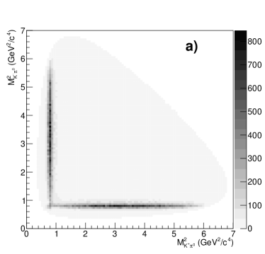
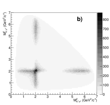
Figure 1: a)-b) Dalitz plots for generated $J/\psi\to K^{*}(892)^{\pm}K^{\mp}\to K^{+}K^{-}\pi^{0}$ and $J/\psi\to K_{2}(1430)^{\mp}K^{\mp}\to K^{+}K^{-}\pi^{0}$ samples correspondingly.

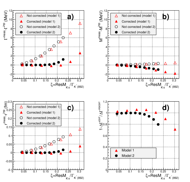
Figure 2: A comparison of fit results when detector resolution is taken into account (solid markers) and ignored (open markers) for $K^{*}(892)$. Results for the first and the second (see in the text) detector response models are shown in red and black correspondingly. Figures a)-c) show fitted width, mass and Blatt-Weisskopf radius, figure d) shows the fraction of width bias due to detector response compensated by the used method. The shown results for the model 2 are limited by $\xi<0.23$ as for higher $\xi$ values using of the quadratic approximation results in non-positive differential cross section for some “data points”.

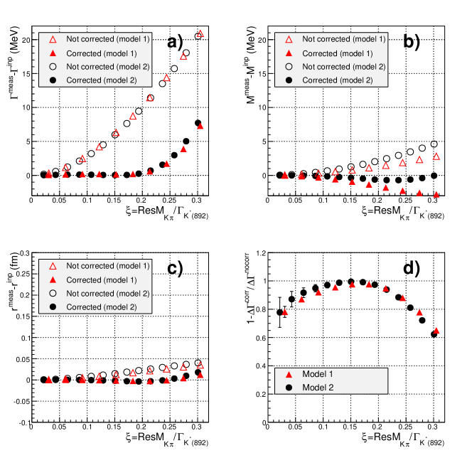
Figure 3: A comparison of fit results when detector resolution is taken into account (solid markers) and ignored (open markers) for $K_{2}(1430)$. Results for the first and the second (see in the text) detector response models are shown in red and black correspondingly. Figures a)-c) show fitted width, mass and Blatt-Weisskopf radius, figure d) shows the fraction of width bias due to detector response compensated by the used method.

6 Conclusion

For the first time we propose a practically acceptable method, which allows in special cases to take into account the detector resolution in the event-by-event partial wave analysis fit. The method reduces the computation of convolution of a process cross section and a detector response function to calculating cross section derivatives and tabulating variances of essential cross section arguments. We demonstrate the method performance and applicability in the set-up of a typical $e^{+}e^{-}$ experiment for two toy detector response models and two reactions: $J/\psi\to K^{*}(892)^{\pm}K^{\mp}\to K^{+}K^{-}\pi^{0}$ and $J/\psi\to K_{2}(1430)^{\pm}K^{\mp}\to K^{+}K^{-}\pi^{0}$.

References

[1]
M. Ablikim et al.,
Nucl. Instrum. Meth. A 614 (2010) 345.
[2]
A. Anisovich, E. Klempt, A. Sarantsev and U. Thoma,
Eur. Phys. J. A 24 (2005) 111.
[3]
K. A. Olive et al.,
Chin. Phys. C 38 (2014) 090001.