Binding energies and spatial structures of small carrier complexes
in monolayer transition metal dichalcogenides via diffusion Monte Carlo

Abstract

Ground state diffusion Monte Carlo is used to investigate the binding energies and carrier probability distributions of excitons, trions, and biexcitons in a variety of two-dimensional transition metal dichalcogenide materials. We compare these results to approximate variational calculations, as well as to analogous Monte Carlo calculations performed with simplified carrier interaction potentials. Our results highlight the successes and failures of approximate approaches as well as the physical features that determine the stability of small carrier complexes in monolayer transition metal dichalcogenide materials. Lastly, we discuss points of agreement and disagreement with recent experiments.

Atomically thin layers of crystalline transition metal dichalcogenides (TMDCs) have been the subject of intense investigation in recent years Splendiani et al. (2010); Mak et al. (2010). As with graphene, TMDCs exhibit remarkable properties that originate from their quasi two-dimensional nature Butler et al. (2013); Geim and Grigorieva (2013). However unlike graphene, TMDCs are direct gap semiconductors, opening up a wealth of potential practical applications ranging from field-effect transistors to photovoltaics Chhowalla et al. (2013); Jariwala et al. (2014). Furthermore, due to the lack of inversion symmetry in these single layer crystals, the so-called $K$-points on opposite corners of the two-dimensional hexagonal Brillouin zone are inequivalent Li and Galli (2007); Lebegue and Eriksson (2009); Gunawan et al. (2006). As a result, a distinct valley degree of freedom associated to states near these points emerges which may be manipulated and controlled, leading to the possibility of novel “valleytronic” applications Mak et al. (2012); Zeng et al. (2012); Xiao et al. (2012); Cao et al. (2012). Lastly, carrier confinement and reduced dielectric screening in these materials leads to large many-body effects, resulting in bound state complexes of electrons and holes with very large binding energies Chernikov et al. (2014); He et al. (2014); Ugeda et al. (2014); You et al. (2015); Mak et al. (2013); Shang et al. (2015); Ross et al. (2013a). In this work we focus on this latter property, providing a deeper understanding of the factors that control the binding energies of electron-hole complexes in two-dimensional TMDCs.

From the computational perspective, the most accurate means of describing excitonic properties in periodic solids currently available is the GW+BSE approach Hybertsen and Louie (1986); Rohlfing and Louie (2000); Cheiwchanchamnangij and Lambrecht (2012); Ramasubramaniam (2012); Qiu et al. (2013). Unfortunately, analogous fully ab initio approaches have not been developed for the treatment of larger electron-hole complexes such as trions and biexcitons You et al. (2015); Mak et al. (2013); Shang et al. (2015); Ross et al. (2013a). However, simplified approaches have proved to be effective, building on well-established coarse-grained methodologies developed for semiconductor quantum wells and other nanostructures. An effective real-space electron-hole potential is combined with an approximate treatment of the band structure, such as an effective mass model or a few-band tight-binding model, to build the model Hamiltonian. This also has roots in the early discussion of the Bethe-Salpeter approach by Hanke and Sham, demonstrating the relationship to the phenomenological approach of Wannier Hanke and Sham (1980).

The pioneering work of Keldysh highlighted the fact that screening effects in quasi two-dimensional systems are intrinsically non-local Keldysh (1979). Using a generalized Keldysh approach, Cudazzo et al. formulated a simple and successful theory for excitons in graphane Cudazzo et al. (2011, 2010). This approach has since been applied by various authors to study optical spectra as well as the properties of excitons, trions, and biexcitons in TMDCs Berkelbach et al. (2013); Berghauser and Malic (2014); Zhang et al. (2014); Fogler et al. (2014); Wang et al. (2014); Wu et al. (2015). These studies have produced exciton binding energies and real-space structures that are in reasonable quantitative agreement with first principles GW+BSE calculations and experiments in a variety of two-dimensional TMDC systems Huser et al. (2013). This fact is not entirely surprising for three reasons. First, recent ab initio calculations show that the effective quasiparticle interactions that emerge at the RPA level nearly perfectly match those used to describe the effective electron-hole interaction in the models mentioned above Steinhoff et al. (2014). Second, the ab initio band structure near the $K$-point is well described by elementary two- and three-band models Xiao et al. (2012); Berkelbach et al. (2015). Third, the spatial extent of the exciton that emerges from fully ab initio calculations is sufficiently large relative to the atomic scale to suggest that a coarse-grained Hamiltonian is justified Ugeda et al. (2014).

Even within the simplified framework of an effective Hamiltonian, the exact solution of the multi-body Schrödinger equation for larger electron-hole complexes is challenging. Initial work on exciton and trion binding energies in TMDCs employed variational wave functions Berkelbach et al. (2013). This approach has been used more recently and with more intricate trial wave functions to study biexcitons You et al. (2015). In both cases the results found from variational solutions of the effective few-body Schrödinger equation are in reasonable agreement with experimental results. However, since binding energies for trions and biexcitons are extracted with reference to the exciton binding energy, the use of variational wave functions for all excitonic complexes leads to binding energies that need not provide a lower bound to the “exact” value, and it is unclear how much error cancellation occurs as a result. For the trion binding energy, Ganchev et al. have discovered a remarkable exact solution, but only for the case where the full Keldysh effective potential is replaced with a completely logarithmic form that is accurate only at short range Ganchev et al. (2015). It is the purpose of this work to investigate the nature and accuracy of these approximate solutions by comparing with numerically exact results, and thereby to provide insights into the properties of higher-order excitonic complexes in two-dimensional TMDCs.

	DMC X (eV)	variational X	DMC X- (meV)	experimental X-	DMC XX (meV)	experimental XX
MoS2	0.5514	0.54	33.8	43 Zhang et al. (2015a), 18 Mak et al. (2013)	22.7	70 Mai et al. (2014)
MoSe2	0.4778	0.47	28.4	30 Ross et al. (2013b)	17.7
WS2	0.5191	0.50	34.0	30 Plechinger et al. (2015), 45 Zhu et al. (2014)	23.3	65 Plechinger et al. (2015)
WSe2	0.4667	0.45	29.5	30 Jones et al. (2013)	20.0	52 You et al. (2015)

Table 1: Estimated exciton (X), trion (X^-), and biexciton (XX) binding energies for different members of the 2D TMDC class of materials. Where two numbers are reported, the number on the left is the most current estimate. The statistical uncertainty in the DMC data is on the order of 0.1–0.3 meV. The column labeled ‘variational’ refers to results based on the Keldysh form, taken from Ref. Berkelbach et al. (2013).

Diffusion Monte Carlo (DMC) provides a useful approach for studying the energetics of excitonic complexes. Briefly, the DMC algorithm propagates an initial wavefunction in imaginary time using a Jastrow-based guiding wavefunction until the exact ground state wavefunction and energy is obtained. Technical details of our DMC calculations can be found in the Supplemental Material. At convergence, DMC yields numerically exact exciton, trion and biexciton ground-state energies within the confines of an effective few-body Schrödinger equation. Specifically, our calculations employ an effective mass treatment of the band structure and an electron-hole interaction appropriate for the two-dimensional TMDC family of materials, i.e.

$$H=-\sum_{i}\frac{\nabla_{i}^{2}}{2m_{i}}+\sum_{i<j}q_{i}q_{j}V(r_{ij})$$ (1)

where

$$V(r)=\frac{\pi}{(\epsilon_{1}+\epsilon_{2})r_{0}}\left[H_{0}(r/r_{0})-Y_{0}(r/r_{0})\right];$$ (2)

in the potential above, $H_{0}$ is the Struve function, $Y_{0}$ is the Bessel function of the second kind, and $\epsilon_{1}$ and $\epsilon_{2}$ are the dielectric constants for the material above and below the TMDC layer; in all results presented, we use $\epsilon_{1}=\epsilon_{2}=1$, relevant for ‘ideal’ or suspended TMDC monolayers.

In addition, DMC allows a full sampling of the square of the wavefunction, which can be used to extract insight into the structure of small bound carrier assemblies. Although DMC has previously been used to calculate ground-state properties for trions interacting with a purely logarithmic potential Ganchev et al. (2015), to the best of our knowledge it has not been used to calculate trion properties with the more realistic electron-hole interaction above, nor has it been used to calculate the properties of biexcitons. It should be noted that while the present work was underway, a numerically exact finite temperature path integral Monte Carlo (PIMC) study of excitons, trions, and biexcitons using the full Keldysh effective potential appeared Velizhanin and Saxena (2015). While we believe that DMC is a more direct method than PIMC for the study of what are essentially ground state properties, we note that the results presented here are in quantitative agreement with those presented earlier in Ref. Velizhanin and Saxena (2015), yielding ground state energies that lie below those of Ref. Velizhanin and Saxena (2015) by fractions of a percent. On the other hand, the goals of this work are somewhat distinct from those of Ref. Velizhanin and Saxena (2015). In particular, we focus on the specific physical factors that influence the delicate balance of relative trion and biexciton binding energies, as well as the accuracy of variational approaches in light of the “exact” DMC results.

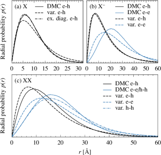
Figure 1: (a) Radial probability distributions for the distance $r_{\textrm{eh}}$ of an exciton in MoS₂; ‘ex. diag.’ refers to the result of a grid-based exact diagonalization. (b) Radial probability distributions for the distances $r_{\textrm{eh}}$ and $r_{\textrm{ee}}$ of a negative trion in MoS₂. (c) Radial probability distributions for the distances $r_{\textrm{eh}}$, $r_{\textrm{ee}}$, and $r_{\textrm{hh}}$ of a biexciton in WSe₂. For the DMC calculation, the curves for $r_{\textrm{ee}}$ and $r_{\textrm{hh}}$ coincide because the electron and hole effective masses are taken to be equal.

	Trion					Biexciton
	Keldysh	pure ln	pure $1/r$	variational 1	variational 2	Keldysh	pure ln	pure $1/r$	variational 1	variational 2
MoS2	33.8	48.9	1630	26	14	22.7	26.2	2610
MoSe2	28.4	39.3	1780	21	12	17.7	21.2	2820
WS2	34.0	53.6	1050	26	14	23.3	28.7	1680
WSe2	29.5	44.9	1120	22	12	20.0	23.9	1780	37	16

Table 2: Comparison of trion and biexciton binding energies for several potential forms in units of meV obtained from DMC, except for the column labeled ‘variational’; the latter results are based on the Keldysh form and taken from Ref. Berkelbach et al. (2013) for trions and Ref. You et al. (2015) for the WSe₂ biexciton. Binding energies in the ‘variational 1’ column are with respect to the variational exciton binding energies, whereas those in the ‘variational 2’ column are with respect to the exact DMC exciton binding energies. For the DMC Keldysh and pure logarithmic potentials, the uncertainty is of the order of 0.1–0.3 meV. For the pure Coulombic potential, the uncertainty is of the order of 10 meV.

In Tab. 1, we report exciton, trion, and biexciton binding energies calculated via DMC and compare to those extracted in recent experiments. The DMC exciton binding energies, defined as $E_{\textrm{b}}^{\textrm{X}}=-E^{\textrm{X}}$, are only 2–4% larger than those obtained in previous variational calculations that employed a trial wavefunction of the form $\Psi_{\textrm{T,var}}(r_{\textrm{eh}})\sim\exp\left(-r_{\textrm{eh}}/a\right)$. The radial probability distribution for the distance $r_{\textrm{eh}}$, which completely determines the exciton wavefunction, is plotted in Fig. 1(a); we compare the variational wavefunction to results obtained via DMC as well as a grid-based exact diagonalization of the one-dimensional Schödinger equation. The simple $1s$-like variational wavefunction matches the true ground-state wavefunction well, but does not decay rapidly enough for large $r$. As we will show, achieving a similar level of agreement between exact DMC and variational estimates for the binding energies of larger excitonic complexes is, in principle, a much more difficult task because trion and biexciton wave functions are more elaborate and their approximation may in principle require many variational parameters to achieve a high level of accuracy.

The DMC trion binding energies given in Tab. 1 are all in the range of 28–34 meV, which is in excellent agreement with current experimental estimates; however it should be noted that realistic substrate effects have been ignored in the present calculations. In Tab. 2, we compare trion binding energies for two additional potentials: a purely logarithmic form and an unscreened $1/r$ Coulombic form. These two potentials represent the asymptotic small and large $r$ behavior, respectively, of (2). The purely logarithmic potential approximation has been employed by Ganchev et al. in their analytical treatment of trions in TMDCs Ganchev et al. (2015) while the Coulomb potential is the standard form for three-dimensional semiconductors. We find that a purely logarithmic potential overbinds the trion and results in binding energies about 50% larger than those reported by experiments. Unsurprisingly, the pure Coulombic potential vastly overbinds the complex, resulting in binding energies that are 30–50 times too large and with a different ordering than is the case for the full potential (2), which is material dependent. Coulombic binding energies would of course be reduced with the inclusion of a static dielectric constant significantly larger than unity.

Our trion binding energies are about 30% larger than those calculated variationally. The two-parameter variational trial wavefunction used in the trion calculations was Berkelbach et al. (2013)

$$\Psi_{\textrm{T,var}}(r_{\textrm{e}_{1}\textrm{h}},r_{\textrm{e}_{2}\textrm{h}})\sim\exp\left(-r_{\textrm{e}_{1}\textrm{h}}/a-r_{\textrm{e}_{2}\textrm{h}}/b\right)+\{a\leftrightarrow b\},$$ (3)

a form inspired by Chandrasekhar’s treatment of the hydrogen anion Chandrasekhar (1944). Although Fig. 1(b) shows that this optimized variational wavefunction reproduces $p(r_{\textrm{eh}})$ almost exactly, the variational form does not capture the electron-electron repulsion properly because it lacks any explicit $r_{\textrm{e}_{1}}-r_{\textrm{e}_{2}}$ correlation terms. The peak of the electron-electron distribution is at too small a radius, which results in over-estimating the electron-electron repulsion and underestimating the trion binding energy, as seen in Tab. 2. Nonetheless, the level of agreement is surprisingly good given the simplicity of the variational wave function employed in Ref. Berkelbach et al. (2013). Furthermore, by treating the exciton and trion on equal footing with physically similar variational wavefunctions, a fortuitous cancellation of total energy errors leads to binding energies which are quite close to the exact results (‘variational 1’ column in Tab. 2); referencing the variational trion energy to the exact DMC exciton energy (‘variational 2’ column in Tab. 2) leads to a significant underestimation of the binding energy, albeit one that is a genuine lower bound.

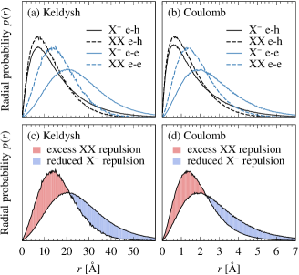
Figure 2: (a) Radial probability distributions for the distances $r_{\textrm{eh}}$ and $r_{\textrm{ee}}$ in the trion (X^-) and biexciton (XX) using a Keldysh form for the inter-carrier potential. (c) The same $r_{\textrm{ee}}$ distributions as in panel (a), but the relocated repulsive weight is shaded. (b),(d) The same as in panels (a),(c) but using a Coulombic form for the inter-carrier potential.

Finally, in Tabs. 1 and 2 we report biexciton binding energies $E_{\textrm{b}}^{\textrm{XX}}=2E^{\textrm{X}}-E^{\textrm{XX}}$ , and in Fig. 1(c) we compare carrier probability distributions obtained from DMC and from a recent six-parameter variational calculation You et al. (2015). Other than the $r_{\textrm{hh}}$ distance, which is accurately predicted, the variational wavefunction is a bit too compact, leading to a total variational energy which is slightly too high. When referenced to the exact DMC exciton energy, we note that the variational biexciton binding energy is actually quite accurate – only 3.5 meV (about 15%) too small. When referenced to the less accurate variational exciton energy, the mis-matched cancellation of errors is such that the biexciton binding energy is slightly overestimated.

In our DMC calculations, we find that the full potential with dielectric screening (2) yields binding energies that are smaller than either of the other potentials considered, and that are smaller than experimental estimates by 60–70%. Most significantly, exact DMC calculations show that the binding energies for biexcitons are significantly smaller than that of trions. This fact, which has been noted in recent PIMC calculations as well Velizhanin and Saxena (2015), disagrees with recent experimental estimates and is at odds with expectations that emerge from the standard case of pure Coulombic interactions. Whereas in the latter $1/r$ case biexcitons are more strongly bound than trions by a factor of about 1.6, in the purely logarithmic case the situation is reversed and trions are more strongly bound than biexcitons. Interestingly, we find that for realistically parameterized Keldysh potentials, the biexciton binding energies are slightly smaller than those found with the purely logarithmic potential, despite the latter being a presumably “weaker” potential; this highlights the subtle balance of energies involved in the formation of the biexciton. We note in passing that the binding energies for biexcitons obtained with the logarithmic potential are significantly closer to the full Keldysh results than they are for trions, suggesting that the short-range approximation of Ganchev et al. may be even better for biexcitons. This result is consistent with the smaller real-space structure of the biexciton seen by comparing Figs. 1(b) and (c).

To gain deeper insight into this balance of energies, we consider the electron-hole and electron-electron distributions for trions and biexcitons obtained with the Keldysh and Coulombic potentials, plotted in Fig. 2(a),(b). Suppose that for a given potential, the attractive electron-hole probability profiles were identical for the trion and the biexciton, and the repulsive electron-electron (hole-hole) profiles were also identical for the trion and the biexciton. Then elementary arguments using the definition of the trion and biexciton binding energies, along with the pairwise additive potential, show that the biexciton binding energy would be exactly twice the trion binding energy, $E_{\textrm{b}}^{\textrm{XX}}/E_{\textrm{b}}^{\textrm{X}^{-}}=2$. Any deviations from this ideal ratio are due to relative differences in the attractive and repulsive probability distributions as the second hole is added to the negative trion.

Instead, biexciton-to-trion binding energy ratios of less than 2 are observed for both the screened interaction (2) and the Coulomb interaction. In both cases, about 9% of the total weight in the $p(r_{\textrm{eh}})$ (attractive) profile is relocated from long $r$ to short $r$. More significantly, a much larger fraction of the total weight in the $p(r_{\textrm{ee}})$ (repulsive) is relocated to short $r$, leading to a reduced biexciton-to-trion ratio. Specifically, for the screened potential (2), about 31% of the weight is relocated, which leads to a biexciton binding energy that is smaller than the trion binding energy; for the Coulomb potential, only 26% of the weight is relocated, and the biexciton binding energy remains larger than the trion binding energy. The relocated repulsive area is shaded for both potentials in Fig. 2(c),(d). From an energetic standpoint, this more notable change in the repulsive profile occurs because in the trion, there is no reason for the like charges to be physically close in space. However, in the biexciton, the complex can achieve stabilizing electron-hole interactions by having the like charges closer together in space.

A final question that may be raised concerns the qualitative difference between biexcitonic stability as found by DMC calculations and that extracted from experiments. As mentioned above, experimentally reported biexciton binding energies significantly exceed experimentally determined trion binding energies, and are about a factor of two or more larger than calculated DMC values. Since our DMC values are exact within the confines of the effective mass and effective potential models, one possibility is that these model ingredients are oversimplified, and need to be amended. Although we have neglected screening from the substrate and surrounding environment, the results of Ref. Velizhanin and Saxena (2015) suggest that the biexciton binding energy will remain less than the trion binding energy, in so far as these latter screening effects can be captured in the effective Keldysh potential. In particular, it is unclear if the assumption of effective pair-wise additive interactions is a good one for larger excitonic complexes; perhaps three-body or higher-order interactions are needed. On the other hand, experimental determination of biexciton binding energies in the TMDCs is quite difficult and involves both assumptions of the nature of spectral signals as well as extrapolations. Clearly future work should be devoted to addressing this interesting discrepancy between theory and experiment.

Note added– Since this work was completed, a preprint has appeared which uses high-accuracy stochastic variational Monte Carlo to calculate the properties of excitons, trions, and biexcitons in monolayer TMDCs Zhang et al. (2015b). The results are in agreement with the present manuscript and the authors further speculate as to the origin of the biexciton discrepancy noted above.

The authors would like to thank Andrey Chaves and Tony F. Heinz for useful discussions. MZM is supported by a fellowship from the National Science Foundation under grant number DGE-11-44155. TCB is supported by the Princeton Center for Theoretical Science. Part of this work was done with facilities at the Center for Functional Nanomaterials, which is a U.S. DOE Office of Science User Facility, at Brookhaven National Laboratory under Contract No. de-sc0012704 (MSH).

Supplemental Material:
Binding energies and spatial structures of small carrier complexes
in monolayer transition metal dichalcogenides via diffusion Monte Carlo

Computational details

In this section we outline the computational approach and model used to investigate excitonic complexes. Our technique of choice is diffusion Monte Carlo (DMC). Because DMC is such a widely used approach, we do not give a detailed account of the method, and refer the reader to more complete technical discussions Needs et al. (2010); Ceperley and Alder (1980); Foulkes et al. (2001).

DMC calculations use the imaginary time Schrödinger equation along with a guiding wavefunction $\Psi_{\textrm{T}}$ to project out excited states from an initial wavefunction $\Phi(t=0)$, propagating it in imaginary time until the true ground state wavefunction $\psi_{0}$ is found. If we define the mixed probability $f(\textbf{R},t)=\Psi_{\textrm{T}}(\textbf{R})\Phi(\textbf{R},t)$ Grimm and Storer (1971); Kalos et al. (1974), where R contains the spatial coordinates of all quantum particles, then the equation of motion for $f(\textbf{R},t)$ derived from the imaginary time Schrödinger equation is

$$-\frac{\partial f(\textbf{R},t)}{\partial t}=-\frac{1}{2}\nabla_{\textbf{R}}^{2}f(\textbf{R},t)+\nabla_{\textbf{R}}\cdot[\textbf{v}(\textbf{R})f(\textbf{R},t)]+(E_{\textrm{L}}(\textbf{R},t)-E_{\textrm{ref}})f(\textbf{R},t),$$ (S1)

where

$$\textbf{v}(\textbf{R},t)=\Psi_{\textrm{T}}^{-1}(\textbf{R})\nabla_{\textbf{R}}\Psi_{\textrm{T}}(\textbf{R}),$$ (S2)

$$E_{\textrm{L}}(\textbf{R})=\Psi_{\textrm{T}}(\textbf{R})^{-1}\hat{H}\Psi_{\textrm{T}}(\textbf{R}),$$ (S3)

and $E_{\textrm{ref}}$ is an arbitrary energy offset. A solution to the importance-sampled imaginary-time Schrödinger equation is then sampled using approximate Greens functions that result in the drift-diffusion motion and the branching action Needs et al. (2010). For the systems we consider, the exact ground state wave function is nodeless, so DMC yields exact ground state energies and a sampling of the exact ground state wavefunctions.

The guiding wavefunction used in this work is of the form $\Psi_{\textrm{T}}(\textbf{R})=e^{J(\textbf{R})}$, which contains the Jastrow factor introduced in Ref. Ganchev et al. (2015) adapted specifically to the potential (2). The Jastrow term contains two-body electron-hole and electron-electron (hole-hole) terms

$$u_{\textrm{eh}}(r)=c_{1}r^{2}\ln(r)e^{-c_{2}r^{2}}-c_{3}r\left(1-e^{-c_{2}r^{2}}\right),$$ (S4)

$$u_{\textrm{ee}}(r)=c_{4}r^{2}\ln(r)e^{-c_{5}r^{2}}.$$ (S5)

The constants $c_{1}=m_{\textrm{e}}m_{\textrm{h}}/2(m_{\textrm{e}}+m_{\textrm{h}})$ and $c_{4}=-m_{\textrm{e}}/4$ ($m_{\textrm{e,h}}$ are the effective masses of the carriers) were chosen to satisfy the logarithmic analogue of the Kato cusp conditions; the other constants were optimized via unreweighted variance minimization to improve the efficiency of the Monte Carlo sampling Umrigar et al. (1988); Drummond and Needs (2005). A blocking method is used to gauge the correlation timescales for the energy estimates, and yields accurate standard deviations for the final average Flyvbjerg and Petersen (1989). Energy estimates were obtained for calculations with $\Delta t\in\{0.01,0.03,0.1\}$, and then extrapolated to zero timestep. All reported DMC probability distributions were sampled from forward-walking DMC calculations Barnett et al. (1991) with the optimal guiding wave function described by Eqs. (S4)–(S5), and $\Delta t=0.01$. A forward walking time of 300 a.u. was used for calculations employing the Keldysh potential; that time was 30 a.u. for calculations using the Coulomb potential.

Screening lengths and effective masses for all materials studied were determined in Ref. Berkelbach et al. (2013). Potentials of the type (2) were first discussed by Keldysh Keldysh (1979) and have been used to treat excitonic properties in quasi two-dimensional materials in several recent studies Cudazzo et al. (2011, 2010); Berkelbach et al. (2013); Berghauser and Malic (2014); Zhang et al. (2014); Fogler et al. (2014); Wang et al. (2014); Wu et al. (2015). The potential (2) behaves as $1/r$ at large $r/r_{0}$, but diverges more weakly as $\ln({r/r_{0}})$ near $r=0$. The crossover point is related to the screening distance $r_{0}=2\pi\chi_{\textrm{2D}}$, where $\chi_{\textrm{2D}}$ is the two-dimensional polarizability of the TMDC layer. For computational efficiency and consistency with past variational calculations, we use a modified form of the effective potential (2), given by

$$V^{\prime}(r)=-\frac{1}{r_{0}}\left[\ln\left(\frac{r}{r+r_{0}}\right)+(\gamma-\ln 2)e^{-r/r_{0}}\right],$$ (S6)

where $\gamma$ is Euler’s constant Cudazzo et al. (2011). Calculations with the unaltered potential (2) typically result in exciton ground-state energies that are merely 2–3 meV lower than those produced with (2).

References

- Splendiani et al. (2010) A. Splendiani, L. Sun, Y. Zhang, T. Li, J. Kim, C. Chim, G. Galli, and F. Wang, Nano Lett. 10, 1271 (2010).
- Mak et al. (2010) K. Mak, C. Lee, J. Hone, J. Shan, and T. F. Heinz, Phys. Rev. Lett. 105, 136805 (2010).
- Butler et al. (2013) S. Z. Butler, S. M. Hollen, L. Y. Cao, Y. Cui, J. A. Gupta, H. R. Gutierrez, T. F. Heinz, S. S. Hong, J. X. Huang, A. F. Ismach, E. Johnston-Halperin, M. Kuno, V. V. Plashnitsa, R. D. Robinson, R. S. Ruoff, S. Salahuddin, J. Shan, L. Shi, M. G. Spencer, M. Terrones, W. Windl, and J. E. Goldberger, ACS Nano. 7, 2898 (2013).
- Geim and Grigorieva (2013) A. K. Geim and I. V. Grigorieva, Nature 499, 419 (2013).
- Chhowalla et al. (2013) M. Chhowalla, H. S. Shin, G. Eda, L. J. Li, K. P. Loh, and H. Zhang, Nat. Chem. 5, 263 (2013).
- Jariwala et al. (2014) D. Jariwala, V. K. Sangwan, L. J. Lauhon, T. J. Marks, and M. C. Hersam, ACS Nano. 8, 1102 (2014).
- Li and Galli (2007) T. S. Li and G. L. Galli, J. Phys. Chem. C 111, 16192 (2007).
- Lebegue and Eriksson (2009) S. Lebegue and O. Eriksson, Phys. Rev. B 79, 115409 (2009).
- Gunawan et al. (2006) O. Gunawan, Y. P. Shkolnikov, K. Vakili, T. Kokmen, E. P. D. Poortere, and M. Shayegan, Phys. Rev. Lett. 97 (2006).
- Mak et al. (2012) K. F. Mak, K. L. He, J. Shan, and T. F. Heinz, Nat. Nano. 7, 494 (2012).
- Zeng et al. (2012) H. L. Zeng, J. F. Dai, W. Yao, D. Xiao, and X. D. Cui, Nat. Nano. 7, 490 (2012).
- Xiao et al. (2012) D. Xiao, G. B. Liu, W. X. Feng, X. D. Xu, and W. Yao, Phys. Rev. Lett. 108, 196802 (2012).
- Cao et al. (2012) T. Cao, G. Wang, W. P. Han, and H. Q. Ye, Nat. Commun. 3, 887 (2012).
- Chernikov et al. (2014) A. Chernikov, T. C. Berkelbach, H. M. Hill, A. Rigosi, Y. Li, O. B. Aslan, D. R. Reichman, M. S. Hybertsen, and T. F. Heinz, Phys. Rev. Lett. 113, 076802 (2014).
- He et al. (2014) K. L. He, N. Kumar, L. Zhao, Z. F. Wang, K. F. Mak, and J. Shan, Phys. Rev. Lett. 113, 026803 (2014).
- Ugeda et al. (2014) M. M. Ugeda, A. J. Bradley, S. F. Shi, F. H. da Jornada, Y. Zhang, D. Y. Qiu, W. Ruan, S. K. Mo, Z. Hussain, Z. X. Shen, F. Wang, S. G. Louie, and M. F. Crommie, Nat. Mater. 13, 1091 (2014).
- You et al. (2015) Y. You, X. Zhang, T. C. Berkelbach, M. S. Hybertsen, D. R. Reichman, and T. F. Heinz, Nat. Phys. 11, 477 (2015).
- Mak et al. (2013) K. F. Mak, K. He, C. Lee, G. H. Lee, J. Hone, T. F. Heinz, and J. Shan, Nat. Mat. 12, 207 (2013).
- Shang et al. (2015) J. Z. Shang, X. N. Shen, C. X. Cong, N. Peimyoo, B. C. Cao, M. Eginligil, and T. Yu, ACS Nano 9, 647 (2015).
- Ross et al. (2013a) J. S. Ross, S. F. Wu, H. Y. Yu, N. J. Ghimire, A. M. Jones, G. Aivazian, J. Q. Yan, D. G. Mandrus, D. Xiao, W. Yao, and X. D. Xu, Nat. Commun. 4, 1474 (2013a).
- Hybertsen and Louie (1986) M. S. Hybertsen and S. G. Louie, Phys. Rev. B 34, 5390 (1986).
- Rohlfing and Louie (2000) M. Rohlfing and S. G. Louie, Phys. Rev. B 62, 4927 (2000).
- Cheiwchanchamnangij and Lambrecht (2012) T. Cheiwchanchamnangij and W. R. L. Lambrecht, Phys. Rev. B 85, 205302 (2012).
- Ramasubramaniam (2012) A. Ramasubramaniam, Phys. Rev. B 86, 115409 (2012).
- Qiu et al. (2013) D. Y. Qiu, F. H. da Jornada, and S. G. Louie, Phys. Rev. Lett. 111, 216805 (2013).
- Hanke and Sham (1980) W. Hanke and L. J. Sham, Phys. Rev. B 21, 4656 (1980).
- Keldysh (1979) L. V. Keldysh, JETP Lett. 29, 658 (1979).
- Cudazzo et al. (2011) P. Cudazzo, I. V. Tokatly, and A. Rubio, Phys. Rev. B 84, 085406 (2011).
- Cudazzo et al. (2010) P. Cudazzo, C. Attaccalite, I. V. Tokatly, and A. Rubio, Phys. Rev. Lett. 104, 226804 (2010).
- Berkelbach et al. (2013) T. C. Berkelbach, M. S. Hybertsen, and D. R. Reichman, Phys. Rev. B 88, 045318 (2013).
- Berghauser and Malic (2014) G. Berghauser and E. Malic, Phys. Rev. B 89, 125309 (2014).
- Zhang et al. (2014) C. J. Zhang, H. N. Wang, W. M. Chan, C. Manolatou, and F. Rana, Phys. Rev. B 89, 205436 (2014).
- Fogler et al. (2014) M. M. Fogler, L. V. Butov, and K. S. Novoselov, Nat. Commun. 5, 4555 (2014).
- Wang et al. (2014) L. Wang, A. Kutana, and B. I. Yakobson, Annalen Der Physik 526, L7 (2014).
- Wu et al. (2015) F. Wu, F. Qu, and A. H. MacDonald, Phys. Rev. B 91, 075310 (2015).
- Huser et al. (2013) F. Huser, T. Olsen, and K. S. Thygesen, Phys. Rev. B 88, 245309 (2013).
- Steinhoff et al. (2014) A. Steinhoff, M. Rosner, F. Jahnke, T. O. Wehling, and C. Gles, Nano Lett. 14, 3743 (2014).
- Berkelbach et al. (2015) T. C. Berkelbach, M. S. Hybertsen, and D. R. Reichman, Phys. Rev. B 92, 085413 (2015).
- Ganchev et al. (2015) B. Ganchev, N. Drummond, I. Aliener, and V. Fal’ko, Phys. Rev. Lett. 114, 107401 (2015).
- Zhang et al. (2015a) Y. Zhang, H. Li, H. Wang, R. Liu, S. Zhang, and Z. Qiu, ACS Nano. Article ASAP, 10.1021/acsnano.5b03505 (2015a).
- Mai et al. (2014) C. Mai, A. Barrette, Y. Yu, Y. G. Semenov, K. W. Kim, L. Cao, and K. Gundogdu, Nano. Lett. 14, 202 (2014).
- Ross et al. (2013b) J. S. Ross, S. Wu, H. Yu, N. J. Ghimire, A. M. Jones, G. Aivazian, J. Yan, D. G. Mandrus, D. Xiao, W. Yao, and X. Xu, Nat. Commun. 4 (2013b).
- Plechinger et al. (2015) G. Plechinger, P. Nagler, J. K. an N. Paradiso, C. Strunk, C. Schuller, and T. Korn, arXiv:1507.01342 (2015).
- Zhu et al. (2014) B. Zhu, H. Zeng, J. Dai, Z. Gong, and X. Cui, Proc. Natl. Acad. Sci. 111, 11606 (2014).
- Jones et al. (2013) A. M. Jones, H. Yu, N. J. Ghimire, S. Wu, G. Aivazian, J. S. Ross, B. Zhao, J. Yan, D. G. Mandrus, D. Xiao, W. Yao, and X. Xu, Nat. Nano. 8, 634 (2013).
- Velizhanin and Saxena (2015) K. Velizhanin and A. Saxena, arXiv:1505.03910v1 (2015).
- Chandrasekhar (1944) S. Chandrasekhar, Astrophys. J. 100, 176 (1944).
- Zhang et al. (2015b) D. K. Zhang, D. W. Kidd, and K. Varga, arXiv:1507.07858 (2015b).

References

- Needs et al. (2010) R. J. Needs, M. D. Towler, N. D. Drummond, and P. L. Rios, J. Phys. Condens. Matter 22, 023201 (2010).
- Ceperley and Alder (1980) D. M. Ceperley and B. J. Alder, Phys. Rev. Lett. 45, 566 (1980).
- Foulkes et al. (2001) W. M. C. Foulkes, L. Mitas, R. J. Needs, and G. Rajagopal, Rev. Mod. Phys. 73, 33 (2001).
- Grimm and Storer (1971) R. C. Grimm and R. G. Storer, J. Comp. Phys. 7, 134 (1971).
- Kalos et al. (1974) M. H. Kalos, D. Levesque, and L. Verlet, Phys. Rev. A 9, 2178 (1974).
- Ganchev et al. (2015) B. Ganchev, N. Drummond, I. Aliener, and V. Fal’ko, Phys. Rev. Lett. 114, 107401 (2015).
- Umrigar et al. (1988) C. J. Umrigar, K. G. Wilson, and J. W. Wilkins, Phys. Rev. Lett. 60, 1719 (1988).
- Drummond and Needs (2005) N. D. Drummond and R. J. Needs, Phys. Rev. B 72, 085124 (2005).
- Flyvbjerg and Petersen (1989) H. Flyvbjerg and H. G. Petersen, J. Chem. Phys. 91, 461 (1989).
- Barnett et al. (1991) R. N. Barnett, P. J. Reynolds, and W. A. Lester, J. Comp. Phys. 96, 258 (1991).
- Berkelbach et al. (2013) T. C. Berkelbach, M. S. Hybertsen, and D. R. Reichman, Phys. Rev. B 88, 045318 (2013).
- Keldysh (1979) L. V. Keldysh, JETP Lett. 29, 658 (1979).
- Cudazzo et al. (2011) P. Cudazzo, I. V. Tokatly, and A. Rubio, Phys. Rev. B 84, 085406 (2011).
- Cudazzo et al. (2010) P. Cudazzo, C. Attaccalite, I. V. Tokatly, and A. Rubio, Phys. Rev. Lett. 104, 226804 (2010).
- Berghauser and Malic (2014) G. Berghauser and E. Malic, Phys. Rev. B 89, 125309 (2014).
- Zhang et al. (2014) C. J. Zhang, H. N. Wang, W. M. Chan, C. Manolatou, and F. Rana, Phys. Rev. B 89, 205436 (2014).
- Fogler et al. (2014) M. M. Fogler, L. V. Butov, and K. S. Novoselov, Nat. Commun. 5, 4555 (2014).
- Wang et al. (2014) L. Wang, A. Kutana, and B. I. Yakobson, Annalen Der Physik 526, L7 (2014).
- Wu et al. (2015) F. Wu, F. Qu, and A. H. MacDonald, Phys. Rev. B 91, 075310 (2015).