Thermal Conductivity in Large-$J$ Two-Dimensional Antiferromagnets: Role of Phonon Scattering

Abstract

Motivated by the recent heat transport experiments in 2D antiferromagnets, such as La₂CuO₄, where the exchange coupling $J$ is larger than the Debye energy $\Theta_{\rm D}$, we discuss different types of relaxation processes for magnon heat current with a particular focus on coupling to 3D phonons. We study thermal conductivity by these in-plane magnetic excitations using two distinct techniques, Boltzmann formalism within the relaxation-time approximation and memory-function approach. Within these approaches, a close consideration is given to the scattering of magnons by both acoustic and optical branches of phonons. A remarkable accord between the two methods with regards to the asymptotic behavior of the effective relaxation rates is demonstrated. Additional scattering mechanisms, due to grain boundaries, impurities, and finite correlation length in the paramagnetic phase, are discussed and included in the calculations of the thermal conductivity $\kappa(T)$. Again, we demonstrate a close similarity of the results from the two techniques of calculating $\kappa(T)$. Our complementary approach strongly suggests that scattering from optical or zone-boundary phonons is important for magnon heat current relaxation in a high temperature window of $\Theta_{D}\lesssim T\ll J$.

I Introduction

After almost three decades of intensive studies, cuprates continue to attract significant interest because of their outstanding properties and due to the continued research effort in high-temperature superconductivity.Ronnow15 ; Kastner98 ; ScalapinoRMP ; Davis ; Vojta ; Basov ; Armitage In particular, their magnetic properties remain inspirational, both as potentially responsible for the mechanism of superconductivityScalapinoRMP and on their own right as relevant to a larger class of low-dimensional antiferromagnets and as a test case for various theoretical models. Ronnow15 ; Greven However, understanding of some of the properties of the magnetic excitations in layered cuprates remains incomplete. This concerns interactions of such excitations with themselves and various other perturbations, as well as the role of such interactions in observable spectroscopic and transport phenomena.

Earlier studies of thermal conductivity in La₂CuO₄ Hess03 ; others have demonstrated large contribution of magnetic excitations to the in-plane thermal transport, thus offering a unique window into their properties which are not easily accessible by other methods. More recent experimental advances Hess15 call for a deeper theoretical insight into the mechanisms of magnon heat current dissipation. This interest goes beyond a particular material and highlights a broader importance of general understanding of the transport phenomena in a wider class of antiferromagnets. While scattering of magnons among themselves and due to fluctuations of the order-parameter in the paramagnetic state has received significant attention in the past,Chubukov the impact of phonons on magnon lifetime and other properties of magnetic excitations has only recently begun receiving attention.Ronnow14

In this context, the current work focuses on the physics of magnon scattering and its role in magnetic thermal transport of quantum antiferromagnets. While our approaches are generic, our analysis is strongly motivated by La₂CuO₄ and related cuprates. Therefore, we concentrate on the case of 2D magnons and superexchange coupling $J$ large compared to the Debye energy $\Theta_{D}$, for temperatures $T\lesssim 0.4J$, where the validity of a magnon description is well-established Takahashi . Moreover, most of our work is devoted to the magnon-phonon scattering to clarify the role of this less-studied relaxation mechanism. Additional effects, such as grain boundary and impurity scattering, and the role of finite correlation length are discussed less extensively.

In addition to investigation of the transport properties of layered cuprates, we also contribute to the formal development of transport theory by contrasting the results from two complementary methods, the Boltzmann theory and the memory function technique. For the relaxation-time approximation within the Boltzmann approach, we take advantage of the large energy scale of magnetic excitations and thus operate with asymptotic, long-wavelength expressions augmented by appropriate cut-offs and some well-justified modeling of the optical phonon spectra. For the magnon-phonon scattering we advocate the use of a simplified “effective phonon DoS” approach, which allows for straightforward yet fairly realistic calculations. In the memory-function approach, on the other hand, we maintain microscopic expressions for the magnon spectra valid in the entire Brillouin zone, while using coupling to a single dispersive phonon branch with a model dispersion, which introduces scattering on both acoustic and optical-like zone-boundary modes. The final results from both approaches, i.e. the thermal conductivities vs. temperature, are found to be remarkably similar. Moreover, a complete agreement between both approaches on the power-law asymptotic regimes, controlled by the optical and acoustic phonons, is also demonstrated.

The paper is organized as follows: we begin with a general discussion of the qualitative features of the magnon-phonon scattering in Sec. II followed by intuitively clear details of Boltzmann approach and calculations of $\kappa(T)$ within it in Sec. III. We continue with the exposition of the memory-function approach and its results for the effective relaxation rates and thermal conductivity in Sec. IV. A brief discussion of other scattering mechanisms and of their respective roles is given in the corresponding sections devoted to the thermal conductivity calculations. Technical details, discussion of the physical range of spin-phonon coupling, etc., are delegated to several Appendices.

II Model and qualitative considerations

Generally speaking, a spin system on a lattice can always be described by a Hamiltonian consisting of spin-only and lattice-only parts, ${\cal H}_{\rm s}$ and ${\cal H}_{\rm ph}$ respectively , in addition to a coupling between them, which we will assume to be of magnetoelastic nature ${\cal H}_{\rm s-ph}$

$${\cal H}={\cal H}_{\rm s}+{\cal H}_{\rm ph}+{\cal H}_{\rm s-ph}={\cal H}_{0}+{\cal H}_{\rm s-ph}\,.$$ (1)

Having in mind La₂CuO₄ and related cuprates, we take a simple, nearest-neighbor-dominated Heisenberg model with the superexchange constant $J$ on a square lattice to be a faithful description of the 2D antiferromagnet of interest. Appendix A offers the standard linear spin-wave treatment of it leading to the free-magnon Hamiltonian

$${\cal H}_{\rm s}\Rightarrow\sum_{\bf k}\varepsilon_{\bf k}\beta^{\dagger}_{\bf k}\beta^{\phantom{{\dagger}}}_{\bf k}\,,$$ (2)

where $\varepsilon_{\bf k}$ is the magnon energy and $\hbar\!=\!k_{B}\!=\!1$ from now on.

The full phonon spectrum of La₂CuO₄ is representative of that of the other cuprates and comprises three acoustic and eighteen optical modes. With a typical bandwidth of each branch from 50K to 400K, together they span the range of energies reaching 900K. Pintschovius91 While in what follows we will model them in a simplified fashion, one can write their Hamiltonian as

$${\cal H}_{\rm ph}\Rightarrow\sum_{{\bf q},\ell}\omega_{{\bf q},\ell}a^{\dagger}_{{\bf q}\ell}a^{\phantom{{\dagger}}}_{{\bf q}\ell}\,,$$ (3)

where $\ell$ numerates branches of phonon excitations.

A straightforward derivation yields the lowest-order magnon-phonon coupling in the following general form (see Appendix B for details)

$${\cal H}_{\rm s-ph}=\sum_{{\bf k,k^{\prime},q}}\sum_{\ell}\Big{\{}V^{\ell}_{\bf k,k^{\prime},q}\beta_{\bf k^{\prime}}^{\dagger}\beta_{\bf k}$$ (4)

$$\phantom{{\cal H}_{\rm s-ph}=}+\frac{1}{2}\,V^{{\rm od},\ell}_{\bf k,k^{\prime},q}\left(\beta_{\bf k^{\prime}}^{\dagger}\beta_{-\bf k}^{\dagger}+\mbox{H.c.}\right)\Big{\}}\left(a^{\dagger}_{{\bf q}\ell}+a_{-{\bf q}\ell}\right),$$

where $V^{\ell}_{\bf k,k^{\prime},q}$ and $V^{{\rm od},\ell}_{\bf k,k^{\prime},q}$ are the “normal” and “anomalous” spin-phonon coupling vertices. For the coupling to acoustic and optical (or zone-boundary) phonons, they assume different asymptotic forms, discussed in the next Section and in Appendix B.

Since we are interested in the thermal transport by magnons, the following generic consideration is useful. Because the phonon Debye energy ($\Theta_{D}\approx 400$K) is much smaller than the magnon bandwidth ($2.2J>3000$K), phonons can be assumed to be in thermal equilibrium, i.e., playing the role of a “bath”. This is well-justified for temperatures comparable to or above half of the phonon Debye energy $T\gtrsim\Theta_{D}/2$, which is about 200K in most cuprates. Then neither the momentum nor the energy of a magnon is conserved in the processes of magnon-phonon scattering, or, in other words, the momentum and energy are transferred from the magnon flow to the phonon bath. In that case, magnon relaxation time and transport times can be treated as the same.

Thus, in contrast to the inter-magnon scattering, the magnon-phonon scattering channel is free from many restrictions of the former and does not have the limitations on the phase space inherent to an Umklapp scenario. While the spin-lattice coupling constant may be small, phonons at temperatures $T>200$K are abundant in the materials of interest.

Another qualitative consideration, elaborated on in Sec. III, is that magnetic excitations are confined to lower dimensions than phonons (i.e., 2D vs 3D). In this case, momentum of phonons perpendicular to the 2D planes is not conserved, which also leads to fewer restrictions on the kinematics of the magnon-phonon scattering.

III Boltzmann approach

III.1 Relaxation rates

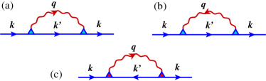
Figure 1: Magnon-phonon scattering diagrams. Solid lines are magnons, wavy lines are phonons. (a) Decay (phonon emission), (b) recombination (phonon absorption), (c) anomalous process (absorption of magnon).

Within the Boltzmann approach, the key element is the calculation of the scattering rates. As is argued above, transport and quasiparticle relaxation rates of magnons due to scattering on phonons should be the same. Then, in the lowest order of spin-phonon coupling, the problem is reduced to evaluation of the diagrams in Fig. 1, which yield magnon relaxation rate by the standard diagrammatic method

$$\frac{1}{\tau_{\bf k}}=\pi\sum_{\bf k^{\prime}}\sum_{{\bf q}_{\parallel}}\sum_{q_{\perp}}$$ (5)

$$\phantom{\frac{1}{\tau_{\bf k}}}\Big{\{}\left|V_{{\bf k},{\bf k^{\prime}},{\bf q}}\right|^{2}\left(n_{\bf q}+n_{\bf k^{\prime}}+1\right)\delta_{{\bf k},{\bf k^{\prime}}+{\bf q}_{\parallel}}\delta\left(\varepsilon_{\bf k}-\varepsilon_{\bf k^{\prime}}-\omega_{\bf q}\right)$$

$$\phantom{\frac{1}{\tau_{\bf k}}}+\left|V_{{\bf k^{\prime}},{\bf k},{\bf q}}\right|^{2}\left(n_{\bf q}-n_{\bf k^{\prime}}\right)\delta_{{\bf k^{\prime}},{\bf k}+{\bf q}_{\parallel}}\delta\left(\varepsilon_{\bf k^{\prime}}-\varepsilon_{\bf k}-\omega_{\bf q}\right)$$

$$\phantom{\frac{1}{\tau_{\bf k}}}+\left|V^{\rm od}_{{\bf k},{\bf k^{\prime}},{\bf q}}\right|^{2}\left(n_{\bf k^{\prime}}-n_{\bf q}\right)\delta_{{\bf k^{\prime}}+{\bf k},{\bf q}_{\parallel}}\delta\left(\varepsilon_{\bf k^{\prime}}+\varepsilon_{\bf k}-\omega_{\bf q}\right)\Big{\}},$$

with the first term corresponding to the diagram in Fig. 1(a), in which phonon is emitted, and the second to Fig. 1(b), in which phonon is absorbed. The third term is due to anomalous process, Fig. 1(c), in which two magnons are absorbed and the phonon is emitted. We drop summation over the phonon branch index $\ell$ here, thus considering one branch of phonons at a time.

The magnon-phonon vertices in (5) are the same as in Eq. (4) and for the first two terms they are related by a permutation of the initial and final states of the magnon. Note that the 2D momentum conservation in Eq. (5), explicated by the $\delta_{{\bf 1},{\bf 2}+{\bf 3}}$’s, concerns only the in-plane momentum of the phonon ${\bf q}_{\parallel}$, while the component perpendicular to the plane, ${\bf q}_{\perp}$, is not conserved. This is natural as magnons have infinite mass in the ${\bf q}_{\perp}$ direction. This feature is important for the future consideration and we separate sums over the components of phonon momenta ${\bf q}=({\bf q}_{\parallel},q_{\perp})$ in Eq. (5) explicitly.

III.2 Approximations

There are two approximations for La₂CuO₄ and related cuprates that follow from the fact that all relevant energies, $T$ and $\Theta_{D}$, are much smaller than the magnon bandwidth, $W\approx 2.2J$: (i) magnon energies can be linearized

$$\varepsilon_{\bf k}\approx v|{\bf k}|,$$ (6)

because for all practical purposes $T\ll J$ and hence $|{\bf k}|\sim T/J\ll 1$, (ii) similarly, magnon-phonon vertices for the optical and acoustic phonons are ($V^{\rm od}_{{\bf k^{\prime}},{\bf k},{\bf q}}\!\approx\!V_{{\bf k},{\bf k^{\prime}},{\bf q}}$)

$$V_{{\bf k},{\bf k^{\prime}},{\bf q}}\approx g_{\rm sp}^{\rm opt}\sqrt{|{\bf k}||{\bf k^{\prime}}|},$$ (7)

$$V_{{\bf k},{\bf k^{\prime}},{\bf q}}\approx g_{\rm sp}^{\rm ac}\sqrt{|{\bf k}||{\bf k^{\prime}}|}\cdot\frac{|{\bf q}_{\parallel}|}{\sqrt{|{\bf q}|}},$$ (8)

where $v$ is the magnon velocity ($v=1.158\sqrt{2}J$, lattice constant $a=1$), and both $g_{\rm sp}^{\rm opt}$ and $g_{\rm sp}^{\rm ac}$ are ${\cal O}(J)\!<J$ (see Sec. III.6 and Appendices B and C for details).Bramwell90 For the acoustic case, the phonon dispersion in the vertex is also linearized, in line with the Debye approximation.

While magnon-phonon vertices in (7) and (8) can be proposed on general grounds, they can also be derived from realistic microscopic models of spin-phonon coupling, an exercise deferred to Appendix B. The same Appendix also deals with the role of polarization of the 3D phonons in the coupling to spins. The asymptotic ${\bf k},{\bf k^{\prime}},{\bf q}\rightarrow 0$ form of these microscopic vertices agrees with (7) and (8), aside from some additional angular dependence that does not affect the results. The typical magnitude of coupling constants $g_{\rm sp}$’s will be discussed in Sec. III.6.

We also make a note that coupling to the optical mode should typically involve a large in-plane momentum transfer ${\bf q}_{\parallel}$, in which case a zone-boundary phonon from the nominally acoustic phonon branch is equivalent to the optical phonon. Such processes result in the scattering of a magnon from, e.g., the branch near ${\bf k}\rightarrow 0$ to another branch near the AF ordering vector ${\bf k^{\prime}}\rightarrow{\bf Q}_{AF}$ [$=(\pi,\pi)$]. Thus, in the following we do not distinguish between the optical and the zone-boundary phonons.

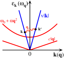
Figure 2: (Color online) Qualitative sketch of the magnon ($\varepsilon_{\bf k}\!=\!v|{\bf k}|$) and acoustic and optical phonon dispersions ($\omega_{\bf q}$’s) in the limit $v\!\gg\!c$. Magnon and acoustic phonon energies are linearized. Schematics of the magnon [momentum ${\bf k}$] absorbing a phonon [in-plane momentum ${\bf q}_{\parallel}$] is also shown.

The next line of approximations requires some qualitative kinematic consideration. The linearization of magnon energies in (6)-(8) is well-justified for a typical $\varepsilon_{\bf k}\!\sim\!T$ and already allows for some simplification in (5). Naturally, the “typical” range of momenta of magnons involved in the heat transport at relevant temperatures is limited by $\simeq\!T/v$, which is $\ll\pi$ and concerns a small fraction of the Brillouin zone. Then, the typical in-plane component of the phonon momenta $|{\bf q}_{\parallel}|\!=\!|\pm{\bf k}\mp{\bf k^{\prime}}|$ for the phonons involved in the magnon scatterings in Fig. 1 must also be limited to the same range, $|{\bf q}_{\parallel}|\!\lesssim\!T/v$, see the sketch in Fig. 2. Note, that if (acoustic) phonons would also be confined to 2D, this would imply that their typical energy needs to be much less than the energy of magnons: $\omega_{\bf q}\!\approx\!c|{\bf q}_{\parallel}|\!\sim\!(c/v)T\!\ll\!T$.

However, for the 3D phonons the situation is radically different. The energy conservations in Eq. (5) imply $\omega_{\bf q}\!=\!|v(|{\bf k}|\pm|{\bf k^{\prime}}|)|$, so for the typical magnon energy $T$, the typical energy of a phonon is also $T$. This, in turn, implies that the out-of-plane component of the phonon momentum is much larger than the in-plane one, $q_{\perp}\!\gg\!|{\bf q}_{\parallel}|$. This is particularly easy to see for the acoustic phonon, for which the combination of the (in-plane) momentum and energy conservations yieldsRC

$$c^{2}\left(|{\bf k}\pm{\bf k^{\prime}}|^{2}+q_{\perp}^{2}\right)=v^{2}\left(|{\bf k}|\pm|{\bf k^{\prime}}|\right)^{2},$$ (9)

so for $|{\bf k}|,|{\bf k^{\prime}}|,|{\bf q}_{\parallel}|\!\sim\!T/v$ it follows that $q_{\perp}\!\sim\!T/c\!\gg\!|{\bf q}_{\parallel}|$. For the optical phonon, $\omega_{\bf q}\!\approx\!\omega_{0}\!+\!\alpha\big{(}\tilde{\bf q}_{\parallel}^{2}+q_{\perp}^{2}\big{)}$, the argument is simply that the typical $|\tilde{\bf q}_{\parallel}|\!\sim\!T/v\!\ll\!1$ while $q_{\perp}$ does not have such restrictions. Note that for the optical phonon $\tilde{\bf q}_{\parallel}\!=\!{\bf q}_{\parallel}\!\pm\!{\bf Q}_{AF}$ is shifted by the in-plane AF-ordering vector.

Altogether, this begs for the following approximation

$$\omega_{\bf q}\approx\omega_{q_{\perp}},$$ (10)

simply neglecting the dependence of the phonon energy on the (small) in-plane momentum transfer $|{\bf q}_{\parallel}|$. This approximation immediately simplifies Eq. (5) as the integral over ${\bf q}_{\parallel}$ simply removes the in-plane momentum delta-functions, while the rest of the expression is independent of it (see a slightly more involved treatment of the case of the acoustic phonon later). Then the integration over ${\bf k^{\prime}}$ in (5) is simply removed by the energy conservation using linearized magnon energies. Lastly, the remaining integration over $q_{\perp}$ can be rewritten by introducing an effective DoS for phonons. Thus, one of the main results of this work is the development of an “effective” approach in which ${\bf k}$- and $T$-dependencies of the relaxation rates in Eq. (5) are given by simple 1D integrals. A very close precision of this approach is demonstrated in Appendix D by a comparison with the direct integration in Eq. (5) without approximation of Eq. (10).

III.3 Effective phonon DoS

After using Eq. (10), the dependence of the integrand in Eq. (5) on $q_{\perp}$ is only through $\omega_{q_{\perp}}$, so it is natural to introduce an “effective” density-of-states of phonons

$$D^{\perp}(\omega)=\sum_{q_{\perp}}\delta\left(\omega-\omega_{q_{\perp}}\right).$$ (11)

We would like to clarify that the “effective” DoS is not the full phonon DoS, but a 1D version of it, which corresponds to the DoS of phonons with the vanishing in-plane momentum.

III.3.1 Optical

Given that the phonon spectrum of cuprates has more than a dosen of optical modes, covering the range from 100K to 900K, Pintschovius91 we reserve the right to model them in a more straightforward fashion. A sketch of such “model” densities of states is shown in Fig. 3. First model, which will be referred to as “Model I”, is just a constant DoS with the gap that corresponds to the lowest optical mode

$$D^{\perp}_{\rm I}(\omega)=\frac{\Theta\left(\omega-\omega_{0}\right)}{\omega_{\rm max}-\omega_{0}}.$$ (12)

The “Model II”, Fig. 3(b), corresponds to the optical mode in the sketch in Fig. 2 with dispersion $\omega_{\bf q}\!=\!\omega_{0}\!+\!\alpha{\bf q}^{2}$ and includes a more realistic square-root singularity at $\omega_{0}$ due to the 1D nature of the “effective DoS” in (11)

$$D^{\perp}_{\rm II}(\omega)=\frac{\Theta\left(\omega-\omega_{0}\right)}{2\pi\sqrt{\alpha(\omega-\omega_{0})}},$$ (13)

with $\alpha\!=\!(\omega_{\rm max}\!-\!\omega_{0})/\pi^{2}$ from normalization. “Model III”

$$D^{\perp}_{\rm II}(\omega)=\delta\left(\omega-\omega_{0}\right),$$ (14)

corresponds to the “flat” optical mode. We would like to note that the results for the thermal conductivity discussed later are remarkably insensitive to the choice of the specific model for the phonon DoS.

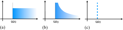
Figure 3: (Color online) Qualitative pictures of the effective DoS for the optical phonons, $D^{\perp}(\omega)$, Eq. (11). (a) “Model I” is the constant with the minimal energy $\omega_{0}$, (b) “Model II”, same with a more realistic square-root singularity at $\omega_{0}$, (c) “Model III” is for the “flat” mode at $\omega_{0}$, Eqs. (12), (13), and (14), respectively.

III.3.2 Acoustic

The effective phonon DoS for the dispersion $\omega_{q_{\perp}}\!=\!cq_{\perp}$ is a constant, same as the “Model I” in (12), but with no gap and an upper cutoff being $\Theta_{D}(\sim\!c)$

$$D^{\perp}_{\rm ac}(\omega)=\frac{1}{\pi c}\Theta\big{(}\Theta_{D}-\omega\big{)}.$$ (15)

The validity of (15) is also restricted from below by $\omega_{\rm min}=(c/v)\varepsilon_{\bf k}$ at which $q_{\perp}\!\approx\!|{\bf q}_{\parallel}|$, as we will discuss later.

III.4 Scattering on the optical phonon

The case of optical phonon is straightforward since magnon-phonon coupling within the approximation (7) does not depend on the phonon momentum. Using linearized form of magnon dispersion and magnon-phonon vertex from (6) and (7), approximation of Eq. (10), and replacing $\sum_{\bf k^{\prime}}$ with $\frac{1}{\pi}\int k^{\prime}dk^{\prime}$ which takes into account two magnon modes per Brillouin zone of the square lattice, yields

$$\frac{1}{\tau_{\bf k}}\approx\left(\frac{g_{\rm sp}^{\rm opt}}{v}\right)^{2}\left(\frac{\varepsilon_{\bf k}}{v^{2}}\right)\int_{0}^{\omega_{\rm max}}d\omega\,D^{\perp}(\omega)$$ (16)

$$\phantom{\frac{1}{\tau_{\bf k}}}\times\Big{\{}\Theta\big{(}\varepsilon_{\bf k}-\omega\big{)}\left(\varepsilon_{\bf k}-\omega\right)^{2}\Big{(}n(\omega)+n(\varepsilon_{\bf k}-\omega)+1\Big{)}$$

$$\phantom{\frac{1}{\tau_{\bf k}}\Big{\{}\Theta\big{(}\varepsilon_{\bf k}-\omega\big{)}}+\left(\varepsilon_{\bf k}+\omega\right)^{2}\Big{(}n(\omega)-n(\varepsilon_{\bf k}+\omega)\Big{)}$$

$$\phantom{\frac{1}{\tau_{\bf k}}\Big{\{}}+\Theta\big{(}\omega-\varepsilon_{\bf k}\big{)}\left(\omega-\varepsilon_{\bf k}\right)^{2}\Big{(}n(\omega-\varepsilon_{\bf k})-n(\omega)\Big{)}\Big{\}},$$

where the first term is from the phonon-emission diagram in Fig. 1(a), the second is due to phonon-absorption in Fig. 1(b), and the third is the anomalous term in Fig. 1(c), first, second, and third terms in Eq. (5), respectively. For the phonon-emission term the phonon energy is limited from above by the energy of the magnon that emits it, $\varepsilon_{\bf k}$, and in the anomalous term the situation is reversed as the phonon energy must exceed that of the magnon, so the integration is limited from below. In (16), $\omega$ is also restricted implicitly through the DoS by $\omega_{0}$, the lowest energy of the optical mode, and by $\omega_{\rm max}$, the highest energy of phonon bands. It is assumed that $\varepsilon_{\bf k}<\omega_{\rm max}$. Thus, after all the legitimate approximations discussed above are implemented, we have a compact expression of the relaxation rate in terms of 1D frequency integrals, Eq. (16). Note that for the “Model III” (flat phonon mode) of the effective phonon DoS this integral in Eq. (16) is trivially removed and the relaxation rate is given by a compact analytical expression, presented in Appendix D.

In the limit of low temperatures, $T,\varepsilon_{\bf k}\!\ll\!\omega_{0}$, phonon-emission term in $1/\tau$ in (16) is strictly zero as the magnon with $\varepsilon_{\bf k}\!<\!\omega_{0}$ cannot emit an optical phonon, and the two remaining terms are exponentially small, $\sim\!e^{-\omega_{0}/T}$.

For higher temperatures $T\!\gtrsim\Theta_{D}$, using the hierarchy of scales $T\!>\!\varepsilon_{\bf k}\!>\!\omega_{0}$ (see Ref. Herring, ) and $n(\omega)\!\simeq\!T/\omega$ yields the asymptotics for the first two terms in (16):

$$\frac{1}{\tau_{\bf k}^{(1)}}\propto\frac{T\varepsilon_{\bf k}^{3}}{v^{2}\omega_{0}}\,,\ \ \ \frac{1}{\tau_{\bf k}^{(2)}}\propto\frac{T^{2}\varepsilon_{\bf k}^{2}}{v^{2}\omega_{0}}\,,$$ (17)

where we used $g_{\rm sp}^{\rm opt}\sim v$. This is valid for Model I and Model II of the effective phonon DoS discussed above, while for the Model III (flat phonon), $1/\tau^{(2)}$ has the same asymptotics $1/\tau^{(1)}$. Although it is natural to expect that the heat is conducted largely by thermalized magnons with a “typical” $\varepsilon_{\bf k}\!\sim\!T$, this is not exactly so in our case, because the distribution of the heat conducting magnons “leans” towards lower energies as we shall discuss later. Nevertheless, it is worth pointing out that “on a thermal shell”, i.e., at $\varepsilon_{\bf k}=T$, where the memory-function and Boltzmann approaches can be consistently compared with each other, both expressions in (17) yield the same

$$\frac{1}{\tau^{\rm opt}}\propto\frac{T^{4}}{v^{2}\omega_{0}}\,.$$ (18)

This coincides with the results of the memory-function approach discussed later. We note that the phonon-emission is always subleading to the absorption term,Herring and the anomalous term is negligible at high $T$.

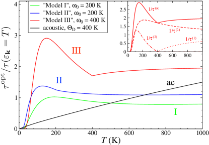
Figure 4: (Color online) $T$-dependence of the magnon relaxation rate on the optical phonons, Eq. (16), for $\varepsilon_{\bf k}\!=\!T$ and using effective phonon DoS models in Eqs. (12)–(14). The results are normalized to the high-temperature asymptotic behavior, Eq. (18), [$T^{4}/v^{2}\omega_{0}$]. Parameters are as discussed in text and indicated in the graph, $\omega_{\rm max}\!=\!950$K for Models I and II. The vertical axis is in units of $(g_{\rm sp}^{\rm opt}/v)^{2}$. Inset shows individual contributions of the three terms in (73) [diagrams in Fig. 1] for Model III. The results for the relaxation rate due to acoustic phonons, Eq. (21), are also shown for a representative choice of the Debye energy $\Theta_{D}\!=\!400$K. $J\!=\!1500$K.

Our Figs. 4 and 14 demonstrate these asymptotic trends explicitly. They also show a close quantitative similarity of the magnon relaxation rates obtained from Eq. (16) using three different models for the effective phonon DoS, Eqs. (12)–(14). In Fig. 4, the $T$-dependence is shown for the relaxation rate for $\varepsilon_{\bf k}\!=\!T$, i.e., on the thermal shell. The results are normalized to $T^{4}/v^{2}\omega_{0}$ to make the high-temperature asymptotic behavior of (18) apparent. The vertical axis is in units of $(g_{\rm sp}^{\rm opt}/v)^{2}$. Inset shows individual contributions of the three terms in (16) for the “Model III” (14). For this model, the contributions of the phonon-emission and anomalous terms [first and third in (73)] are explicitly limited by the step-functions, resulting in a kink at $T\!=\!\omega_{0}$, while for the other models these are smoothed out. For the sake of a comparison with the acoustic phonons in the next Section, we also note that the results for the scattering on the optical phonon in Figs. 4 and 14 likely underestimate the effect by a numerical factor about 2, due to scattering of magnons between ${\bf k}\rightarrow 0$ and ${\bf k}\rightarrow{\bf Q}_{AF}$ branches.

III.5 Acoustic phonon

Below we demonstrate that the effective phonon DoS approach can be successfully extended to the consideration of magnon scattering off the acoustic phonons.

The crucial difference of the acoustic phonon scattering is the form of the magnon-phonon coupling in Eq. (8), which leads to an extra factor $|{\bf q}_{\parallel}|^{2}/|{\bf q}|$ in the scattering probability compared with the optical phonon case. A naïve power-counting, together with the kinematic consideration in Sec. III.2 suggest that the typical $|{\bf q}_{\parallel}|\!\sim\!T/v$ while $|{\bf q}|\!\approx\!q_{\perp}\!\approx\!(v/c)|{\bf q}_{\parallel}|$, translating this extra factor into $cT/v$ for the relaxation rate. Using that the phonon sound velocity $c\!\sim\!\Theta_{D}\!\sim\!\omega_{0}$, this would yield the “thermal shell” estimate for the relaxation rate $1/\tau^{\rm ac}\!\sim\!T^{5}/v^{4}$, to be contrasted with the asymptotic expression for the optical case (18). The situation is more delicate, however, as the scattering in the present case is, in fact, dominated by the low-$\omega$ phonons. Technically, the integral over the phonon energies diverges as $1/\omega$ and must be cut off at $\omega_{\rm min}\!=\!(c/v)\varepsilon_{\bf k}$, where $q_{\perp}$ becomes $\approx\!|{\bf q}_{\parallel}|$. Altogether, assuming $g_{\rm sp}^{\rm ac}\!\sim\!v$, this gives the “thermal shell” estimate for the acoustic case as

$$\frac{1}{\tau^{\rm ac}}\propto\frac{T^{5}}{\Theta_{D}v^{3}},$$ (19)

which is valid for both $T\!>\!\Theta_{D}$ and $T\!<\!\Theta_{D}$. Note, that the result (19) is the same as in the memory-function consideration, Sec. IV.

A rigorous derivation of this result from Eq. (5) needs a slightly more delicate treatment of the magnon-phonon coupling. We use $|{\bf q}_{\parallel}|^{2}\!=\!|{\bf k^{\prime}}\!-\!{\bf k}|^{2}$ and, according to approximation in Eq. (10), $|{\bf q}|\!\approx\!q_{\perp}$. Then the extra factor $|{\bf q}_{\parallel}|^{2}/|{\bf q}|$ in the scattering probability reads

$$\frac{|{\bf k^{\prime}}|^{2}+|{\bf k}|^{2}-2|{\bf k^{\prime}}||{\bf k}|\cos\varphi}{q_{\perp}}\Rightarrow\left(\frac{c}{v^{2}}\right)\left(\frac{\varepsilon_{\bf k^{\prime}}^{2}+\varepsilon_{\bf k}^{2}}{\omega_{q_{\perp}}}\right),$$ (20)

where $\varphi$ is the angle between ${\bf k^{\prime}}$ and ${\bf k}$ and, because of the approximation of Eq. (10), the term with $\cos\varphi$ averages to zero upon the integration over this angle. With the result in Eq. (20) and using the effective DoS model for the acoustic branch introduced in Eq. (15), we rewrite the relaxation rate in (5) as

$$\frac{1}{\tau^{\rm ac}_{\bf k}}\approx\left(\frac{g_{\rm sp}^{\rm ac}}{v}\right)^{2}\left(\frac{c\,\varepsilon_{\bf k}}{v^{4}}\right)\int_{\omega_{\rm min}}^{\Theta_{D}}d\omega\,\frac{D_{\rm ac}^{\perp}(\omega)}{\omega}\,\Big{\{}\Theta\big{(}\varepsilon_{\bf k}-\omega\big{)}\ \ \$$ (21)

$$\times\left(\left(\varepsilon_{\bf k}-\omega\right)^{4}+\varepsilon_{\bf k}^{2}\left(\varepsilon_{\bf k}-\omega\right)^{2}\right)\Big{(}n(\omega)+n(\varepsilon_{\bf k}-\omega)+1\Big{)}$$

$$+\left(\left(\varepsilon_{\bf k}+\omega\right)^{4}+\varepsilon_{\bf k}^{2}\left(\varepsilon_{\bf k}+\omega\right)^{2}\right)\Big{(}n(\omega)-n(\varepsilon_{\bf k}+\omega)\Big{)}$$

$$+\Theta\big{(}\omega-\varepsilon_{\bf k}\big{)}$$

$$\times\left(\left(\omega-\varepsilon_{\bf k}\right)^{4}+\varepsilon_{\bf k}^{2}\left(\omega-\varepsilon_{\bf k}\right)^{2}\right)\Big{(}n(\omega-\varepsilon_{\bf k})-n(\omega)\Big{)}\Big{\}},$$

where the three terms are the phonon-emission, phonon-absorption, and anomalous terms in Fig. 1(a)-(c) and in Eq. (5), and $\omega_{\rm min}\!=\!(c/v)\varepsilon_{\bf k}$ as before.

We first note that the contribution of the anomalous term in the acoustic phonon case of Eq. (21) is by a factor of $c/v$ smaller than that of the other two terms. The subtle reason for that is in the threshold nature of the process: the lowest possible phonon energy is $\varepsilon_{\bf k}$, not $\omega_{\rm min}$, which gives the thermal-shell estimate $1/\tau^{(3)}\!\sim\!T^{5}/v^{4}$, much less than the result in (19). We, therefore, give the asymptotic consideration only to the first two terms.

Because the integral over the phonon energy in (21) is infrared-divergent and thus is dominated by the low-energy phonons, the asymptotic behavior of both terms is the same at low and high temperatures ($T\!<\!\Theta_{D}$ and $T\!>\!\Theta_{D}$). For $\varepsilon_{\bf k}$ being of the same order as $T$, both terms in (21) yield an estimate of the relaxation rate

$$\frac{1}{\tau_{\bf k}^{(1)}}\approx\frac{1}{\tau_{\bf k}^{(2)}}\sim\left(\frac{g_{\rm sp}^{\rm ac}}{v}\right)^{2}\left(\frac{T\varepsilon_{\bf k}^{4}}{v^{3}c}\right),$$ (22)

which is in accord with the thermal-shell answer (19). As we discuss below, the phonon-absorption term has a more complicated $\varepsilon_{\bf k}$-dependence for $\varepsilon_{\bf k}\!\ll\!T$.

The asymptotic result (19) should be compared with the high-temperature ($T\!>\!\omega_{0}\!\sim\!\Theta_{D}$) estimate for the optical phonon case, Eq. (18). The ratio of (19) to the latter is $T/v$, which should imply that the contribution of the scattering on acoustic phonons is a relatively minor effect in this temperature regime. A direct comparison is provided in Fig. 4, where the black line is obtained from (21), without the use of the asymptotics. This line clearly indicates that the asymptotic consideration of Eqs. (19) and (22) is correct and that the relaxation rate on thermalized acoustic phonons follows $T^{5}$ power law.

On a closer inspection of Fig. 4 we should note, first, that the dominance of the acoustic phonon scattering in the low-$T$ regime concerns a really small region of $T\!\lesssim\!\Theta_{D}/4$ and is unlikely to be seen in the thermal conductivity of La₂CuO₄ as this regime is known to be dominated by the grain-boundary scattering.Hess03 Second, at the higher $T$, the relaxation rate by acoustic phonons seems to exceed the one by optical phonons, at least for some of the models of their DoS. This is likely to be due to a neglect of the numerical factor difference in the coupling strength to acoustic and optical phonons in our effective vertices (8) and (7), and an underestimate of the optical phonon scattering rate by a numerical factor mentioned in Sec. III.4.

III.6 Summary of the phonon-scattering mechanisms

Here we would like to summarize our considerations of the magnon-phonon scattering and to take a broader view of its implication for the thermal conductivity.

III.6.1 Smallness of $g$’s

First, while the perturbative character of our treatment of magnon-phonon scattering is implied by the use of the lowest Born approximation in Fig. 1 and Eq. (5), we would like to make it explicit that the physical range of the phenomenological magnon-phonon constants we introduce in (7) and (8) is $g_{\rm sp}/v\!\ll\!1$. At first glance this may be surprising as the dependence of the superexchange constants on the interatomic distance is often rather sharp and is governed by some high power of the distance, leading to estimates $\partial J/\partial a\!\approx\!\gamma J$ with $\gamma\!\sim\!10-20$, see Ref. Bramwell90, . However, this largeness is offset by the smallness of a characteristic atomic displacement associated with phonons,Bramwell90 $1/\sqrt{m\Theta_{D}}\!\sim\!1/100$, see Appendices B and C on how the two factors appear together within a microscopic approach.

III.6.2 $k$-dependence

Second, we note the importance of the $\varepsilon_{\bf k}$-dependence of the relaxation time. For bosons with $\varepsilon_{\bf k}\!\approx\!v|{\bf k}|$, one can estimate thermal conductivity asHerring ; RC

$$\kappa\propto\int_{0}^{T/v}\tau_{\bf k}d{\bf k}\,.$$ (23)

According to the preceding sections, in magnon-phonon $1/\tau_{\bf k}$ the lowest power is $k^{2}$. In a similar situation in 1D,RC this leads to a strong infrared divergence of the spin component of the thermal conductivity. This means that the spin-phonon scattering is not sufficient to render conductivity finite and one needs to take into consideration other scattering mechanisms. In 2D, the integral in (23) still has a weak (logarithmic) divergence for $\tau\!\sim\!k^{-2}$, so the (grain-)boundary scattering is sufficient to mitigate it. One of the implications of this is that the distribution of magnons that carry the heat most effectively is not centered at energies of order $T$, but is shifted toward lower energies. More importantly, this consideration means that with the $\varepsilon_{\bf k}$-dependence of the relaxation rates obtained in Secs. III.4 and III.5, magnon-phonon scattering cannot be the only scattering mechanism and thus must be accompanied by a boundary-like scattering in order to render magnon heat conductivity finite.

III.6.3 Effective $1/\tau$

Lastly, given how close the results for different models of the phonon spectra conform to the asymptotic expressions for $1/\tau_{\bf k}$ in (17) and (22), it is tempting to introduce a simplified, “effective” expression for the magnon relaxation rate on optical and acoustic phonons that contains a minimal number of parameters

$$\frac{1}{\tau_{\bf k}^{\rm eff}}\approx\sum_{i}a^{\rm opt}_{i}\,\widetilde{\Theta}\left(T-\widetilde{\omega}_{0,i}\right)\frac{T^{2}k^{2}}{\omega_{0,i}}+a^{\rm ac}\,\frac{vTk^{4}}{\Theta_{D}},$$ (24)

where $a^{\rm ac}\!\equiv\!(g_{\rm sp}^{\rm ac}/v)^{2}$ and $a^{\rm opt}_{i}\!\equiv\!(g_{{\rm sp},i}^{\rm opt}/v)^{2}$ are the dimensionless coupling constants to the acoustic and the $i$th optical mode which has the (lowest) energy $\omega_{0,i}$. The “pseudo”-step-function $\widetilde{\Theta}(x)$ is introduced to mimicTheta the exponential “turn-on” of the scattering on optical modes at the temperatures $T$ around $\widetilde{\omega}_{0,i}\!=\!\omega_{0,i}/2$, as in Fig. 4.

We remark that thermal conductivity obtained with this effective $1/\tau_{\bf k}$ and appropriate set of parameters can be made virtually indistinguishable from the ones using more elaborate expressions from Secs. III.4 and III.5.

III.7 Other scattering mechanisms

III.7.1 Grain-boundary

As is discussed in previous section, boundary scattering is essential to mitigate residual infrared divergence of magnon $\kappa_{m}$ if only scattering on phonons is considered. One can expect that in a 2D magnetic lattice even relatively weak dislocation-like defects are likely to act as strong boundaries for magnon propagation, similarly to the effect of crystal grain boundaries on phonons. Experimentally, the grain-boundary scattering is known to dominate entirely the low-temperature ($T\!\lesssim\!200$K) magnon thermal conductivity of La₂CuO₄.Hess03 The corresponding relaxation rate is simply

$$\frac{1}{\tau_{\bf k}^{\rm b}}\approx\frac{v}{L},$$ (25)

where $L$ is the characteristic size of the grain. The typical grain size quoted in Ref. Hess03, is $L\!\sim\!150$ lattice spacings and is in agreement with the other measurements in La₂CuO₄.

III.7.2 Correlation length

In the paramagnetic state above the Néel temperature, which is non-zero in most unfrustrated 2D AFs because of the interplane interactions and/or small anisotropies, finite spin-spin correlation length can be expected to represent a natural “cut-off” boundary for magnon propagation because magnons are the spin-flips in an ordered structure. This expectation is in agreement with a number of studies which have pointed out that the dynamics of the antiferromagnets is fully diffusive at scales beyond the correlation length $\xi(T)$, i.e., that the propagating magnons are overdamped by fluctuations at distances $\lambda\!\gtrsim\!\xi(T)$.HH ; CHN ; Grempel ; Tyc In effect, the correlation length acts a temperature-dependent size of an order-parameter domain for magnon propagation.

The exponential dependence of the 2D correlation length on $J/T$ has been verified experimentally in La₂CuO₄ and in the other 2D antiferromagnets,Kastner98 ; Goff ; Ronnow and is supported by extensive theoretical and numerical Quantum Monte-Carlo (QMC) calculations.CHN ; Makivic ; Hasenfratz00 An approximate analytical expression of it for the spin-$\frac{1}{2}$, nearest-neighbor Heisenberg antiferromagnet on a square lattice isGreven

$$\xi(T)=\frac{1.13J}{2.26J+T}\,e^{1.13J/T},$$ (26)

in units of lattice spacings. While it was argued that the characteristic length-scale that defines magnon lifetime should also contain a temperature-dependent prefactorCHN ; Grempel ; Makivic ; Goff as well as correctional factors, Hasenfratz00 we simply suggest the following scattering rate by interpreting correlation length as a mean-free path

$$\frac{1}{\tau_{\bf k}^{\xi}}\approx\frac{v}{\xi(T)}.$$ (27)

These seemingly naive expression and expectation are supported by the studies of the $T$-dependence of the magnon linewidth in copper-formate-tetradeuterate (CFTD), another model spin-$\frac{1}{2}$ square-lattice antiferromagnet, by inelastic neutron scattering and QMC.Ronnow In fact, the relaxation rate in the form of Eq. (27) has been suggested in Ref. Ronnow, , which has demonstrated that in both experiment and QMC results the magnon linewidth is well described by (27) at $T\!\gtrsim\!0.2J$.

Another effect of the finite correlation length is an effective gap $\Delta_{\xi}\!=\!v/2\xi$ in the magnon spectrumTakahashi

$$\varepsilon_{\bf k}\approx v\sqrt{k^{2}+\xi^{-2}(T)/4},$$ (28)

which, obviously, affects the contribution of the long-wavelength excitations to thermal conductivity.

III.7.3 Lattice disorder

In a recent study,Ronnow14 the following scenario has been put forward. Since the ionic motion in the cuprates is much slower than the superexchange processes among spins, the former must cause a significant variation of couplings $J$ due to zero-point and thermal lattice fluctuations. The effect was estimated from the high-resolution neutron diffraction and the zero-point motion was found responsible for the distribution of the width $\delta J\!\sim\!0.1J$.Ronnow14 In a sense, this implies that magnons propagate in a medium with the velocity that is randomly varying around the mean value with a distribution given by $\delta J(T)$. One can approximate this effect by the $T$-dependent static random lattice disorder with the lowest-order magnon relaxation rate due to this mechanism given by

$$\frac{1}{\tau_{\bf k}^{\rm lat}}\approx\frac{\delta J^{2}(T)}{J}\,k^{3}\,,$$ (29)

where the temperature-dependent disorder strength can be modeled as $\delta J(T)\!=\!\delta J(0)\sqrt{1+4T/\Theta_{D}}$ to interpolate between the amplitude of zero-point and temperature-induced lattice fluctuations within the Debye approximation.Ziman ; Ronnow14

Related to this mechanism are two other possible sources of magnon scattering at high temperatures that are harder to estimate. First is specific to La₂CuO₄, which exhibits orthorhombic-to-tetragonal structural phase transition at about 525K associated with a softening of a phonon mode.Kastner98 This transition may have a direct impact on the values of superexchange constants and also enhance magnon-phonon scattering involving the mode that is being softened. However, it is hard to quantify both without a microscopic insight.

Second is a significant decrease and eventual collapse of $J$ at high enough temperatures, advocated in Ref. Bramwell90, as an ultimate result of the thermal expansion. With the large value of $J$ and an apparent insignificant impact of the expansion on the average value of $J$ in the $0-300$K rangeRonnow14 in La₂CuO₄, it is hard to estimate at what $T$ such dramatic effects can be expected to onset.

III.7.4 Magnon-magnon scattering

Last but not the least is the effect of magnon-magnon scattering. Since these require an explicit momentum dissipation to contribute to conductivities, the standard Umklapp process leading to a scattering of a typical low-energy magnon with the momentum $k$ must involve a high-energy magnon with the energy $\varepsilon_{\rm max}\!\approx\!2.2J$. Then, one can suggest an ansatz

$$\frac{1}{\tau_{\bf k}^{\rm mm,U}}\approx Jk\,e^{-2.2J/T}\,.$$ (30)

This can be seen as an upper limit estimate for the standard Umklapp scattering rate as it neglects possible smallness of the matrix element and only takes into account the smallness of $k$ from the initial state.

There exists a possibility of an unconventional “low-energy Umklapp”, because magnons in La₂CuO₄ have two branches, at ${\bf k}=(0,0)$ and ${\bf k}=(\pi,\pi)$, so that some of the scattering between these branches may carry away large momenta. This logic seems to be implied in a recent calculation in Ref. Keimer, . In that case, the corresponding relaxation rate can be expected to display a power-law behavior, similar to the “normal” magnon-magnon scatteringChubukov

$$\frac{1}{\tau_{\bf k}^{\rm m-m}}\sim\frac{T^{2}k}{v}\,,$$ (31)

which, on “thermal shell”, differs by a factor $T/\omega_{0}$ from the magnon-phonon estimate in (18). This implies that for sufficiently high temperatures, $T\gg\omega_{0}$, magnon-phonon scattering must be more important than the inter-magnon scattering.

Moreover, this expression must carry a small prefactor as it neglects the smallnesses of the fraction of the Umklapp vs normal processes and of the phase space for scattering. The apparent inability of the magnon-magnon scattering theory of Ref. Keimer, to fit the data for La₂CuO₄ from Ref. Hess03, beyond the boundary-controlled regime can be seen as an indirect evidence of the relative unimportance of this type of scattering for the magnon thermal conductivity in large-$J$ materials. We thus exclude it from the subsequent consideration.

III.7.5 Comparison

To gain a qualitative expectation for the relative contribution of the discussed scattering mechanisms in different temperature regimes, we compile the results from Eqs. (24), (25), (27), (29), and (30) in our Fig. 5, which shows relaxation rates normalized to the high-$T$ asymptote of the optical-phonon scattering in (18) [$1/\tau^{\rm opt}\!=\!T^{4}/v^{2}\Theta_{D}$], as in Fig. 4. For the magnon-phonon scattering (24) we have dimensionless coupling constants $a^{\rm opt}_{1}\!=\!a^{\rm ac}\!=\!0.1$ and $a^{\rm opt}_{2}\!=\!0.3$ with $\omega_{0,1}\!=\!\Theta_{D}\!=\!400$K and $\omega_{0,2}\!=\!900$K. For the boundary scattering (25) the scattering length is $L\!=\!300$ lattice spacings, and for the correlation length effect (27) we use the expression for $\xi(T)$ in Eq. (26). Temperature-dependent lattice disorder coupling in (29) is chosen with $\delta J(0)\!=\!0.1J$ to roughly match the results of Ref. Ronnow14, . $J\!=\!1500$K as before and magnon energy $\varepsilon_{\bf k}$ is chosen to be $\varepsilon_{\bf k}\!=\!4T$, the value of energy which roughly corresponds to the maximum of the thermal population of magnons at a given $T$.

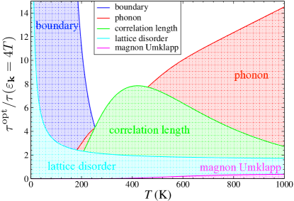
Figure 5: (Color online) Magnon relaxation rates from Eqs. (24), (25), (27), (29), and (30) normalized to $T^{4}/v^{2}\Theta_{D}$, Eq. (18), at $\varepsilon_{\bf k}\!=\!4T$. Parameters are as described in text.

One can see in Fig. 5 that the scattering at low-$T$ ($T\!\lesssim\!\Theta_{D}/2$) is controlled entirely by the grain boundaries. We note that the magnon-phonon scattering and the lattice-disorder scattering have a substantial dependence on $\varepsilon_{\bf k}$ and thus lead to a stronger scattering for magnons with $\varepsilon_{\bf k}\!>\!T$, but to a weaker scattering for $\varepsilon_{\bf k}\!<\!T$. Thus, in Fig. 5 at intermediate and high-$T$ ($T\!\gtrsim\!\Theta_{D}/2$) the dominant contribution is due to finite correlation length and phonons. The magnon-phonon scattering is at least as strong as the scattering due to correlation length at intermediate $T$ and even exceeds it for the higher $T$ for the given choice of $\varepsilon_{\bf k}$. While lattice disorder effect is also significant, it remains secondary and, given its nearly perfect $T^{4}$ asymptotic behavior, may be incorporated into the magnon-phonon coupling to an optical mode. Thus, while the lower-energy magnons are scattered almost exclusively by the boundaries and finite correlation length, at $T\!\gtrsim\!\Theta_{D}$ the higher-energy magnons are strongly scattered by phonons.

Altogether, grain-boundary, correlation length, and magnon-phonon scatterings are the leading mechanisms of magnon energy relaxation and, therefore, have to be included in the consideration of thermal conductivity offered next.

III.8 Thermal conductivity

Within the Boltzmann formalism thermal conductivity by bosonic excitations in 2D is

$$\kappa=\sum_{\bf k}\left(\cos\varphi\,v_{\bf k}\right)^{2}\left(\frac{\varepsilon_{\bf k}}{T}\right)^{2}\left(n_{\bf k}^{2}+n_{\bf k}\right)\,\tau_{\bf k}\,,$$ (32)

where $\varphi$ is the angle between ${\bf v}_{\bf k}$ and the current. Using the linearized form of magnon dispersion (6) and the fact that all of the discussed relaxation rates are isotropic in ${\bf k}$ we can simplify (32) to a 1D integral

$$\kappa\approx\frac{T^{2}}{2\pi}\int_{0}^{x_{\rm max}}dx\,\frac{x^{3}\,e^{x}}{(e^{x}-1)^{2}}\,\tau(x,T)\,,$$ (33)

where $x\!=\!\varepsilon_{\bf k}/T$ and $x_{\rm max}\!=\!\varepsilon_{\rm max}/T$ with $\varepsilon_{\rm max}\!=\!v\sqrt{2\pi}$, in which we used the Debye-like approximation for magnons and also accounted for two magnon modes in the Brillouin zone.

At finite correlation length $\xi$, the magnon spectrum opens a gapTakahashi according to (28), which results in a modification of the expression for the thermal conductivity

$$\kappa\approx\frac{T^{2}}{2\pi}\int_{x_{\rm min}}^{x_{\rm max}}dx\left(1-\frac{x^{2}_{\rm min}}{x^{2}}\right)\,\frac{x^{3}\,e^{x}}{(e^{x}-1)^{2}}\,\tau(x,T)\,,$$ (34)

where $x_{\rm min}\!=\!\Delta_{\xi}/T$ with $\Delta_{\xi}\!=\!v/2\xi(T)$.

III.8.1 Comparison

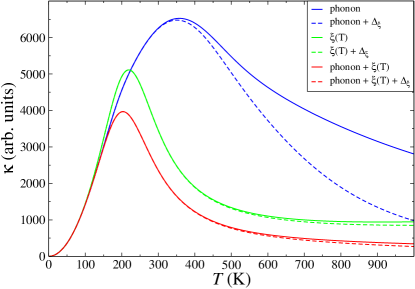
Figure 6: (Color online) Magnon $\kappa(T)$ for the scattering by the grain boundaries, $L\!=\!300$, and either the correlation length (middle curves), Eq. (27), or phonon scattering (upper curves), Eq. (24). Lower curves combine the effects of all three, grain-boundary, phonon, and correlation length scattering mechanisms. Parameters for the phonon scattering are as in Fig. 5. Dashed lines show the effect of the gap in magnon spectrum (34).

Finally, we present the results of our calculations of magnon thermal conductivity in Figs. 6 and 7, in which we demonstrate the effects of boundary scattering (25) together with the finite correlation length and/or magnon-phonon relaxation mechanisms. In Fig. 6, the upper solid curve shows $\kappa(T)$ for the case when the scattering is only by the grain boundaries (25) with $L\!=\!300$ and by phonons (24) with the same coupling parameters as in Fig. 5. The middle solid curve is for $\kappa(T)$ due to grain boundaries (25) and the correlation length (27). The corresponding dashed lines are for the same cases, but with an additional effect of the finite-$T$ gap in the magnon spectrum $\Delta_{\xi}$ due to finite correlation length, Eq. (34). The effect is minimal on the middle curve, but is rather dramatic in the phonon-scattering case. This is due to strong $\varepsilon_{\bf k}$-dependence of the magnon-phonon scattering discussed in Sec. III.7, which changes substantially the magnon population contributing to the heat current. Namely, in the “boundary+$\xi(T)$” case, the typical magnon in (34) is a thermalized one, $\varepsilon_{\bf k}\!\sim\!T$, so the exponentially small gap $\Delta_{\xi}(T)$ of (28) does not affect it. In the “boundary+phonon” case, the high-energy magnons are scattered strongly by phonons, see Fig. 5, while the heat-conducting population of magnons leans strongly to the low energies, hence a dramatic impact of opening the gap.

Lower curves shows the result of combining all three, the grain-boundary, the phonon, and the correlation length scattering mechanisms. Clearly, the phonon relaxation mechanism leads to a stronger scattering at the higher-$\varepsilon_{\bf k}$ part of the heat-conducting magnon population, reducing the overall conductivity, while the longer-wavelength part is now controlled by the correlation length, evidenced by a weak sensitivity of $\kappa(T)$ to the gap in the magnon spectrum (dashed curves).

Fig. 7 complements this study with the consideration of three different scenarios: the magnon-phonon coupling is to (i) two optical modes, one at $\omega_{0,1}\!=\!400$K and the other at $\omega_{0,2}\!=\!900$K (an analog of the high-energy stretching mode), (ii) to an acoustic branch of phonons only, and (iii) to both (same curve as in Fig. 6). One can see that the overall effect on $\kappa(T)$ is very similar in all three cases. This is natural in the light of the preceding discussion that points to the significant scattering effect by phonons at higher energies, which can be expected to be comparable regardless of the nature of the phonon branches. We would also like to point out that we have performed the same calculation of $\kappa(T)$ in (34) using not the “effective” magnon-phonon relaxation rate, proposed in Sec. III.6 in Eq. (24), but the relaxation rates in Secs. III.4 and III.5, Eqs. (16) and (21), using different effective phonon DoS models, previously matched to a direct numerical integration in Eq. (5). Aside for the adjustments of the magnon-phonon coupling constants needed in the cases when phonon spectral weight is spread over a substantial energy range, these calculations have produced the results that are virtually identical to the ones in Figs. 6 and 7.

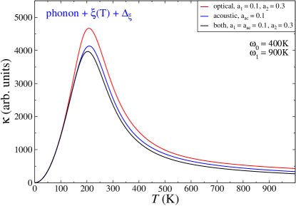
Figure 7: (Color online) Magnon $\kappa(T)$ with all three key scatterings, same as in Fig. 6. For the magnon-phonon scattering, results for coupling to only optical, only acoustic, and to both are shown.

Altogether, magnon thermal conductivity in La₂CuO₄ should be largely controlled by the “boundary-like” scatterings, coming from either the real grain-boundaries or the 2D correlation length, with a substantial correction from the magnon-phonon scattering, affecting $\kappa(T)$ at intermediate and high temperatures.

III.8.2 Remarks

For the latter regime, there are two additional remarks that need to be made. First, according to Eq. (26), at 800K ($\approx\!0.5J$) the correlation length is of order of 3 lattice spacings. Is the magnon picture still applicable and is it realistic to expect further reduction of the mean-free path by a phonon scattering? We believe that although the magnon description at $T\!\gtrsim\!0.5J$ may be an extrapolation, such a correlation length corresponds to a “patch” of about 30 spins, which is known to be well-described by the spin-waves in finite-cluster studies. A somewhat more relevant quantity is the effective gap in the magnon spectrum at this temperature, $\Delta_{\xi}\!\approx\!J/4$, which is still considerably smaller than the magnon bandwidth ($2J$). Given that the magnon-phonon scattering mostly affects magnons with $\varepsilon_{\bf k}\!>\!T$, it seems perfectly legitimate that the phonons are the source of a further shortening of the mean-free path in this regime.

Second, the use of the bosonic description of the thermodynamics of spin excitations of the $S\!=\!\frac{1}{2}$ Heisenberg model on a square lattice is limited by the temperatures of order $0.6J$, at which the specific heat shows a broad maximumSandvik_Cv while within the bosonic description specific heat saturates at a somewhat higher $T$. For a comparison of our results with experimental data this implies that the high-temperature tail of our $\kappa(T)$ should only serve as an upper limit estimate of the reality.

IV Memory function approach

We now turn to the memory function approach, which does not proceed via one particle excitations, but focuses on the dynamics of the current directly, as we will sketch next. We start from the magnon heat current in terms of Bogoliubov quasiparticles

$$\mathbf{j}=\sum_{\mathbf{k}}\varepsilon_{\mathbf{k}}\mathbf{v}_{\mathbf{k}}\beta_{\mathbf{k}}^{\dagger}\beta_{\mathbf{k}}^{\vphantom{\dagger}}\,,$$ (35)

where $\mathbf{v}_{\mathbf{k}}=\nabla_{\mathbf{k}}\varepsilon_{\mathbf{k}}$ is the velocity of the magnon. Following the memory function method Forster1975 , the dynamical thermal conductivity tensor at frequency $z=\omega+i0^{+}$ is

$$VT\kappa_{\mu\nu}{=}\left\langle j_{\mu}\left|\frac{i}{z-{\cal L}}\right.j_{\nu}\right\rangle{=}\left(\frac{i}{z-\mathbf{M}(z){\bm{\chi}}^{-1}}\bm{\chi}\right)_{\mu\nu},$$ (36)

where $V$ is the volume, and ${\cal L}={\cal L}_{{\rm s}}+{\cal L}_{{\rm ph}}+{\cal L}_{{\rm s-ph}}={\cal L}_{0}+{\cal L}_{{\rm s-ph}}$ is the Liouville operator ${\cal L}A=[{\cal H},A]$, comprising spin, phonon, and spin-phonon parts, see (1). $\langle A|B\rangle=\int_{0}^{\beta}\langle A^{+}(\lambda)B\rangle d\lambda-\beta\langle A^{+}\rangle\langle B\rangle$ is the Mori’s scalar product with $A(\lambda)=e^{\lambda{\cal H}}Ae^{-\lambda{\cal H}}$ and $\beta=1/T$ is the inverse temperature. $\bm{\chi}$ is the isothermal heat current susceptibility, $\chi_{\mu\nu}=\langle j_{\mu}|j_{\nu}\rangle$, and $M_{\mu\nu}(z)=\langle{\cal L}j_{\mu}|(z-Q{\cal L})^{-1}Q{\cal L}j_{\nu}\rangle$ is the memory function matrix. $Q$ is a projector perpendicular to the heat current in terms of Mori’s product $Q=1-\sum_{\mu\nu}|j_{\mu}\rangle\chi_{\mu\nu}^{-1}\langle j_{\nu}|$.

We will evaluate (36) for $\omega\rightarrow 0$ to order $O({\cal H}_{{\rm s-ph}}^{2})$. Within perturbation theory Forster1975 to the leading order in the spin-phonon coupling, the memory matrix is given by

$$M_{\mu\nu}(z)=\left\langle[{\cal H}_{{\rm s-ph}},j_{\mu}]\left|\frac{1}{z-{\cal L}_{0}}\right.[{\cal H}_{{\rm s-ph}},j_{\nu}]\right\rangle_{0}\,,$$ (37)

where the subscript $0$ refers to Mori’s product and thermal averaging with respect to the canonical ensemble of the system at zero coupling, ${\cal H}_{{\rm s-ph}}=0$. This subscript will be dropped hereafter. Since $M_{\mu\nu}\sim O({\cal H}_{{\rm s-ph}}^{2})$ already, the static current susceptibility is needed only for ${\cal H}_{{\rm s-ph}}=0$. With $[{\cal H}_{0},j_{\mu}]=0$ and $\langle j_{\mu}\rangle=0$

$$\chi_{\mu\nu}=\frac{\delta_{\mu\nu}}{T}\langle j_{x}j_{x}\rangle=\frac{\delta_{\mu\nu}}{2T}\sum_{\mathbf{k}}\varepsilon_{\mathbf{k}}^{2}\mathbf{v}_{\mathbf{k}}^{2}n(\varepsilon_{\mathbf{k}})\left(1+n(\varepsilon_{\mathbf{k}})\right)\,,$$ (38)

where $n(\varepsilon_{\mathbf{k}})=1/(e^{\varepsilon_{\mathbf{k}}/T}-1)$ is the Bose-function.

IV.1 Relaxation time approximation

The relaxation-time approximation corresponds to replacing $\mathbf{M}(z)/\bm{\chi}$ by $-i/\tau$ with a phenomenological scattering time $\tau$. In that case (36) reads

$$\kappa=\frac{1}{2T^{2}}\sum_{\mathbf{k}}\varepsilon_{\mathbf{k}}^{2}\mathbf{v}_{\mathbf{k}}^{2}n(\varepsilon_{\mathbf{k}})\left(1+n(\varepsilon_{\mathbf{k}})\right)\,\tau\,,$$ (39)

with $\kappa_{\mu\nu}=\delta_{\mu\nu}\kappa$. This is identical to the standard result from kinetic theory. For $T\ll J$, Eq. (39) yields $\kappa\propto T^{2}$, as expected for bosons in $2D$. While the case $T\gg J$ is unphysical, we note that then $\kappa\propto const$.

We note that (39) is completely identical to (32) for a momentum-independent scattering rate. In principle, the memory function approach in Eq. (36) can be formulated with a particle-hole type of observable, $\mathbf{j}_{\mathbf{kq}}=\varepsilon_{\mathbf{k}}\mathbf{v}_{\mathbf{k}}\beta_{\mathbf{k}}^{\dagger}\beta_{\mathbf{k}+\mathbf{q}}^{\vphantom{\dagger}}$, in order to explicitly analyze momentum-dependent current relaxations rates. We will not pursue this direction here.

IV.2 Spin-phonon relaxation rate

Here we would like to restrict ourselves to the case of acoustic phonons. This reduces the problem to a monoatomic Bravais lattice with ionic masses $m$ where magnetoelastic couplings results from stretching of the nearest-neighbor exchange bonds along the in-plane bond directions, the case considered in detail in Appendix B. Lattice deformations perpendicular to the bond direction lead to higher-order couplings.

First, we use explicit form of ${\cal H}_{{\rm s-ph}}$ in (4) to find the commutator $[{\cal H}_{{\rm s-ph}},j_{\mu}]$, which has a meaning of a force

$$[{\cal H}_{{\rm s-ph}},j_{\mu}]=\frac{1}{2N}\sum_{\mathbf{k}{\mathbf{q}},\ell}B_{\mathbf{k^{\prime}}}^{\dagger}\,\mathbf{F}_{\mathbf{k},\mathbf{q}}^{\ell\mu}\,B_{\mathbf{k}}^{\vphantom{\dagger}}\,\left(a_{-{\mathbf{q}}\ell}^{\dagger}+a_{{\mathbf{q}}\ell}^{\vphantom{\dagger}}\right)\,,$$ (40)

where ${\bf k^{\prime}}={\bf k}+{\bf q}_{\parallel}$ imposed by the conservation of the in-plane component of the momentum, $\ell$ numerates acoustic phonon branches, $B_{\mathbf{k}}^{\dagger}=(\beta_{\mathbf{k}}^{\dagger},\beta_{\mathbf{k}}^{\vphantom{\dagger}})$, and the matrix

$$\mathbf{F}_{\mathbf{k},\mathbf{q}}^{\ell\mu} = \left(e_{\mathbf{k}}^{\mu}-e_{\mathbf{k}+\mathbf{q}_{\parallel}}^{\mu}\right)\mathbf{V}_{\mathbf{k},{\bf k}+{\bf q}_{\parallel},{\mathbf{q}}}^{\ell}\,,$$ (41)

where we have introduced the shorthand notation for the energy current of a single magnon mode $\mathbf{e}_{\mathbf{k}}=\varepsilon_{\mathbf{k}}\mathbf{v}_{\mathbf{k}}$ and used inversion symmetry $\varepsilon_{-\mathbf{k}}=\varepsilon_{\mathbf{k}}$, $\mathbf{v}_{-\mathbf{k}}=-\mathbf{v}_{\mathbf{k}}$. The $2\times 2$ “vertex matrix” $\mathbf{V}_{\mathbf{k},{\bf k^{\prime}},{\mathbf{q}}}^{\ell}$ is built from the diagonal elements responsible for the “normal” scattering processes, $V_{{\bf k,k^{\prime},q}}^{\ell}$ given in (62), and the off-diagonal, “anomalous” terms $V_{{\bf k,k^{\prime},q}}^{{\rm od},\ell}$ given in (63).

As usual Forster1975 (37) can be rewritten as $z\,M_{\mu\nu}(z)=\chi_{\mu\nu}^{F}(z)-\chi_{\mu\nu}^{F}$, where $\chi_{\mu\nu}^{F}(z)$ is the retarded dynamical force-force susceptibility, resulting from analytic continuation of the imaginary-time Greens function $\chi_{\mu\nu}^{F}(\tau)=\langle T_{\tau}([{\cal H}_{{\rm s-ph}},j_{\mu}]^{+}(\tau)[{\cal H}_{{\rm s-ph}},j_{\mu}])\rangle$, and $\chi_{\mu\nu}^{F}=\langle[{\cal H}_{{\rm s-ph}},j_{\mu}]|[{\cal H}_{{\rm s-ph}},j_{\mu}]\rangle$ is the isothermal force-force susceptibility. Due to tetragonal symmetry, all of these quantities are diagonal with respect to $\mu,\nu$.

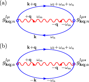
Figure 8: (Color online) Force-force susceptibility diagrams. Solid lines are magnons, wavy lines are phonons. (a) normal contribution (magnon emission-absorption), (b) anomalous contribution (two magnon emission (absorption)). Filled circles in (a) are normal and in (b) anomalous force-vertices.

For thermal transport we focus on the DC limit $\omega{\rightarrow}0$. Since $\mathrm{Re}[M_{\mu\nu}(i0^{+})]=0$ and $\mathrm{Im}\chi_{\mu\nu}^{F}=0$, we have to calculate $\mathrm{Im}[\chi_{\mu\nu}^{F}(z=i0^{+})]$ only. This can be done using the two diagrams in Fig. 8, which comprise normal magnon emission-absorption and anomalous two-magnon emission (absorption) processes, i.e. $\chi_{\mu\nu}^{Fn}(z)$ and $\chi_{\mu\nu}^{Fa_{1,2}}(z)$. After some algebra we get

$$M_{\mu\nu}(i0^{+})=-i\,\frac{\pi\delta_{\mu\nu}}{T}\sum_{\mathbf{k},{\mathbf{q}},\ell}n(\omega_{\mathbf{q}}^{\ell})$$

$$\times\Big{(}2|g_{\mathbf{k}{\mathbf{q}};n}^{\ell\mu}|^{2}n(\varepsilon_{\mathbf{k}})\left(1{+}n(\varepsilon_{\mathbf{k}+\mathbf{q}_{\parallel}})\right)\delta\left(\varepsilon_{\mathbf{k}}{-}\varepsilon_{\mathbf{k}+\mathbf{q}_{\parallel}}{+}\omega_{\mathbf{q}}^{\ell}\right)$$

$$+|g_{\mathbf{k}{\mathbf{q}};a}^{\ell\mu}|^{2}\big{(}1{+}n(\varepsilon_{\mathbf{k}})\big{)}\left(1{+}n(\varepsilon_{\mathbf{k}+\mathbf{q}_{\parallel}})\right)\delta\left(\varepsilon_{\mathbf{k}}{+}\varepsilon_{\mathbf{k}+\mathbf{q}_{\parallel}}{+}\omega_{\mathbf{q}}^{\ell}\right)\Big{)},$$

where the “force vertices” $g_{\mathbf{k}{\mathbf{q}};n(a)}^{\ell\mu}$ refer to the normal (subscript $n$) and anomalous (subscript $a$) processes

$$g_{\mathbf{k}{\mathbf{q}};n}^{\ell\mu}=\left(e_{\mathbf{k}}^{\mu}-e_{\mathbf{k}+\mathbf{q}_{\parallel}}^{\mu}\right)\,V_{{\bf k},{\bf k}+{\bf q}_{\parallel},{\bf q}}^{\ell},$$ (43)

$$g_{\mathbf{k}{\mathbf{q}};a}^{\ell\mu}=\left(e_{\mathbf{k}}^{\mu}-e_{\mathbf{k}+\mathbf{q}_{\parallel}}^{\mu}\right)\,V_{{\bf k},{\bf k}+{\bf q}_{\parallel},{\bf q}}^{{\rm od,\ell}},$$ (44)

with the explicit expressions for vertices given in (62) and (63). We note that $\mathrm{Im}[M_{\mu\mu}^{n(a)}(i0^{+})]\leqslant 0$ separately for both normal and anomalous contributions, as to be expected from causality.

IV.3 Phonon dispersion

In the following sections we provide a discussion of several aspects of thermal conductivity obtained from the memory function approach. We are going to discuss orders of magnitude estimates for the cuprates, the asymptotic behavior of the scattering rate, and the results from the numerical evaluation of the memory function. Whenever of interest, explicit reference will be made to parameters relevant to La₂CuO₄. In what follows, we parametrize phonon excitations that are relevant for spin-phonon coupling as given by two degenerate modes that are polarized in-plane and have the dispersion

$$\omega^{\ell}_{{\mathbf{q}}}=\Theta_{D}\,\sqrt{\sum_{\alpha}\sin\left(\frac{q_{\alpha}}{2}\right)^{2}}\,.$$ (45)

$\Theta_{D}$ is the Debye energy for phonons as before. Since we set $\hbar=k_{B}=1$ and also assume all lengths in units of lattice constant unless mentioned otherwise, $\Theta_{D}/2$ and the sound velocity $c$ will be used interchangeably.

IV.4 Asymptotic scattering rates

For the “normal” emission-absorption of acoustic phonons in Fig. 8(a) we expect four asymptotic temperature regimes, which are determined in part by the kinematics of the magnon-phonon scattering. (i) For $T\ll\Theta_{D}$, thermalized magnon-phonon scattering involves only long-wavelength excitations. (ii) As $T$ is increased, scattering from the zone-boundary, optical-like phonons with $\omega_{{\mathbf{q}}}\lesssim T$ and a high density of states begin contribute with the Arrhenius-like, activated $T$-dependence. For the dispersion in (45) such phonons occur at the corners of the BZ at $\mathbf{q}\sim\mathbf{Q}_{AF}=(\pi,\pi)$. (iii) For $\omega_{\mathbf{Q}_{AF},q_{\perp}}\ll T\ll J$, magnons can be scattered by thermalized phonons from $\mathbf{k}\!=\!(0,0)$ to $\mathbf{Q}_{AF}$. (iv) Finally, one can consider a regime $T\gg J$ in (IV.2), which however is unphysical regarding the definition of magnons.

IV.4.1 Acoustic phonon regime

First, we consider the “normal” scattering processes and $T\ll\Theta_{D}$. For that we may use the long-wavelength limit $|\mathbf{k}+\mathbf{q}_{\parallel}|,|{\bf k}|,|{\bf q}_{\parallel}|\!\ll\!1$ for all the in-plane wave vectors. As discussed in detail in Appendix B, the in-plane modulation of $J$ will only couple to the two out of three phonon branches, whose in-plane polarization can be always chosen as $|$$\xi$${}_{{\bf q}}^{\ell}|\!\approx\!1$. We also approximate $\omega_{{\mathbf{q}}}^{\ell}\!\approx\!c|{\bf q}|\!=\!c\sqrt{|{\bf q}_{\parallel}|^{2}+|{\bf q}_{\perp}|^{2}}$, with a sound velocity much less then the magnon velocity, i.e. $c\ll v$. Expanding in (43) to lowest order in $|\mathbf{k}+\mathbf{q}_{\parallel}|$, $|{\bf k}|$, and $|{\bf q}_{\parallel}|$, the memory function reads

$$M_{\mu\nu}(i0^{+})=-i\,\delta_{\mu\nu}\frac{2\pi\left(g_{{\rm sp}}^{{\rm ac}}\right)^{2}}{T}$$

$$\hphantom{M_{\mu\nu}(i0^{+})}\times\sum_{\mathbf{k},\mathbf{q},\ell}\frac{|{\bf q}_{\parallel}|^{2}|{\bf k}||\mathbf{k}+\mathbf{q}_{\parallel}|\left(e_{\mathbf{k}}^{\mu}-e_{\mathbf{k}+\mathbf{q}_{\parallel}}^{\mu}\right)^{2}}{\sqrt{|{\bf q}_{\parallel}|^{2}+|{\bf q}_{\perp}|^{2}}}$$

$$\hphantom{aa}\times n(\omega_{\mathbf{q}}^{\ell})n(\varepsilon_{\mathbf{k}})\left(1{+}n(\varepsilon_{\mathbf{k}+\mathbf{q}_{\parallel}})\right)\delta\left(\varepsilon_{\mathbf{k}}{-}\varepsilon_{\mathbf{k}+\mathbf{q}_{\parallel}}{+}\omega_{\mathbf{q}}^{\ell}\right),$$

where $g_{{\rm sp}}^{{\rm ac}}\!=\!S\lambda/(2\sqrt{mc})$ with $\lambda\!=\!\partial J/\partial r$, see Appendix B and Eq. (65). First, the magnon and phonon distribution functions $n(\varepsilon_{\mathbf{k}})$ and $n(\omega_{\mathbf{q}}^{\ell})$ in (IV.4.1) imply that $|{\bf k}|\!\sim\!T/v$ and $|{\bf q}|\!\sim\!T/c$. From this and using energy conservation $\varepsilon_{\mathbf{k}+\mathbf{q}_{\parallel}}\!=\!\varepsilon_{\mathbf{k}}\!+\!\omega_{\mathbf{q}}^{\ell}$, we conclude that the in-plane phonon momentum is of magnitude $|\mathbf{q}_{\parallel}|\!\sim\!T/v$, i.e. the dominant contribution of the phonon momentum is out-of-plane. This coincides with the conclusion reached in Sec. III.2 after Eq. (9). In turn, $|\mathbf{k}+\mathbf{q}_{\parallel}|\!\sim\!T/v$ and $(e_{\mathbf{k}}^{\mu}-e_{\mathbf{k}+\mathbf{q}_{\parallel}}^{\mu})^{2}\!\sim\!v^{2}T^{2}$. Then, a naïve power-counting, accounting also for factors of magnon and phonon velocities, $v$ and $c$, and keeping in mind that the $\delta(\ldots)$-function in (IV.4.1) replaces one $k$-integration by a factor of $1/v$, suggests that $M\!\sim\!(g_{{\rm sp}}^{{\rm ac}})^{2}T^{8}/v^{6}$. However, this approach misses one subtle detail, i.e. that the $q_{\perp}$-integration is singular with

$$\int_{0}^{T/c}dq_{\perp}\frac{n(\omega_{\mathbf{q}}^{\ell})}{\sqrt{|{\bf q}_{\parallel}|^{2}+|{\bf q}_{\perp}|^{2}}}\sim\int_{T/v}^{T/c}dq_{\perp}\frac{T}{cq_{\perp}^{2}}\sim\frac{v}{c}\,,$$ (47)

which introduces an additional factor of $(v/c)$ and finally leads to

$$M_{\mu\nu}^{n}(i0^{+})\propto-i\,\delta_{\mu\nu}\left(g_{{\rm sp}}^{{\rm ac}}\right)^{2}\,\frac{T^{8}}{cv^{5}}\,.$$ (48)

From (38) we have $\chi_{\mu\nu}\sim T^{3}$ with a dimensionless prefactor of order unity. Therefore, using $c\sim\Theta_{D}$, the scattering rate is

$$\frac{1}{\tau_{ac}^{n}}\propto\frac{T^{5}}{\Theta_{D}v^{3}}\,,$$ (49)

with the dimensionless prefactor $\left(g_{{\rm sp}}^{{\rm ac}}/v\right)^{2}$. This result is identical to our Eq. (19) and the discussion is completely in line with the consideration given in Sec. III.5.

IV.4.2 Zone-boundary phonon regime and others

We now consider the normal scattering processes from the optical-like, zone-boundary phonons with ${\bf q}_{\parallel}\approx(\pi,\pi)$. First, we focus on temperatures $J\!\gg\!T\!\gg\!\omega_{0}\!\approx\!\Theta_{D}$. Calculations are simplified by shifting the zero of the planar component of the phonon momentum to the edge of the BZ, i.e. ${\bf q}_{\parallel}\rightarrow{\bf q}_{\parallel}+(\pi,\pi)$, and therefore $\mathbf{q}\rightarrow\mathbf{q}+(\pi,\pi,0)$. Since $T\!\ll\!J$, one can still expand in (43) with respect to small momenta $|\mathbf{k}+\mathbf{q}_{\parallel}|$ and $|{\bf k}|$ near their respective ${\bf k}$-points in the BZ, while for phonons one can set $\omega_{\mathbf{q}}^{\ell}\!\sim\!\omega_{0}$ for all ${\bf q}$ involved in the scattering. Using this expansion for vertices as discussed in Appendix B, one can easily see that it leaves the structure of the expression for the memory function in (IV.4.1) almost intact, with the only difference that both ${\bf q}$ and ${\bf q}_{\parallel}$ are large. Then, the power counting proceeds the same way as above with all the variables related to magnons governed by the same smallness of the typical momentum $k\sim T/v$, while for the phonon occupation number we now have $n(\omega_{\mathbf{q}}^{\ell})\!\sim\!T/\omega_{0}$ and the summation over $q_{\perp}$ has no restrictions. Altogether, this yields

$$M_{\mu\nu}^{n}(i0^{+})\propto-i\,\delta_{\mu\nu}\left(g_{{\rm sp}}^{{\rm zb}}\right)^{2}\,\frac{T^{7}}{\omega_{0}v^{4}}\,,$$ (50)

where $g_{{\rm sp}}^{{\rm zb}}\!=\!4S\lambda/\sqrt{2m\Theta_{D}}$ as given in (69). Similarly to the acoustic case, this implies the following scattering rate

$$\frac{1}{\tau_{opt}^{n}}\propto\frac{T^{4}}{\omega_{0}v^{2}}\,,$$ (51)

in a complete agreement with the relaxation rate obtained in Sec. III.4, Eq. (18).

Without repeating similar considerations for the anomalous scattering in Fig. 8(b), we simply note that the numerical evaluation to be presented in the next subsection shows that for experimentally relevant temperatures $T\gtrsim 0.1\Theta_{D}$ its contribution is smaller by several orders of magnitude as compared to normal scattering.

Finally, we note that in the unphysical regime of $T\!\gg\!J$, the memory function scales as $M\sim T^{2}$ due to the three distribution functions and the prefactor of $1/T$. Together with $\chi_{\mu\nu}\sim T$ for this regime, this yields a relaxation rate of $\tau^{-1}\propto T$.

Figure 9: (Color online) Difference quotient $n=\Delta\ln[M_{\mu\nu}(i0^{+})]/\Delta\ln T$ obtained from numerical evaluation of $M_{\mu\nu}(i0^{+})$ versus $T$ (dots) for various $\Theta_{D}$ (lines are guides to the eye). Error bar is an estimated maximum “error”: $n-\partial\ln[M_{\mu\nu}(i0^{+})]/\partial\ln T$. For reference note that for $J=1550$K, $\Theta_{D}=0.1J$ corresponds to a maximum phonon energy of approximately $270$K.

IV.5 Numerical analysis of the memory function

Figure 9 sheds light on our asymptotic analysis of relaxation rates from an unbiased numerical point of view. The memory function has been evaluated using Eqs. (IV.2) and (45) for three representative Debye energies $\Theta_{D}$. The numerical integration has been set up to satisfy the energy conserving delta-function exactly through the numerical solution of $\varepsilon_{\mathbf{k}+\mathbf{q}}=\varepsilon_{\mathbf{k}}+\omega_{\mathbf{q}}^{\ell}$ for each integrand call. This leaves a 4D integration with a non-trivial integrand. Evaluation of the latter has been performed for the temperatures shown by the dots in Fig. 9. It shows a numerical approximation to $\partial\ln[M_{\mu\nu}(i0^{+})]/\partial\ln T$, the quantity which allows to clearly identify the temperature ranges where the memory matrix follows a power law, $M_{\mu\nu}(i0^{+})\propto T^{n}$. These ranges can be seen as plateaus with the heights directly giving the exponent $n$.

We would like to stress several points. First, as predicted, a clear $T^{8}$ regime, corresponding to $\tau^{-1}\propto T^{5}$, can be observed for $T\ll\Theta_{D}$. However, comparing with the energy scales appropriate for La₂CuO₄, such a regime is unlikely to be observed in the current experimental studies of it, because the scattering in this temperature range is dominated by the grain boundaries. Hess03 Second, while this may be an artifact of our scheme of modeling the optical phonon scattering by the phonon spectrum with a single phonon branch, for a robust $T^{7}$ ($\tau^{-1}\propto T^{4}$) regime to occur, the Debye energy needs to be low enough compared to $J$. This is evident from the set of data in Fig. 9 with $\Theta_{D}=0.1J$ where clear indications of the $T^{7}$ range can be observed. However, it is obvious from the results for $\Theta_{D}=0.2J$ and $\Theta_{D}=0.3J$, that this regime rapidly merges with the onset of thermalization of the high-energy magnons, where no well-defined exponent can be observed. Third, the increase of the exponent between the $T^{8}$ and the $T^{7}$ regimes is consistent with an exponential increase of $M_{\mu\nu}(i0^{+})$ with temperature. This is exactly the signature of the Arrhenius (activated) behavior mentioned as regime (ii) in Sec. IV.4. Finally, as expected for $T\gg J$ we get $M_{\mu\nu}(i0^{+})\propto T^{2}$.

IV.6 Thermal conductivity

In this subsection we combine the memory function analysis of the spin-phonon coupling with the scattering mechanisms discussed in Sec. III.7 that are most significant for magnon thermal transport in large-$J$ antiferromagnets such as La₂CuO₄. Moreover, we will use parameters that may provide a reasonable description of the experimental thermal conductivity data, e.g. of Ref. Hess03, . To leading order, additional scattering mechanisms can be added according to the Matthiessen’s rule, i.e. summing their respective momentum-independent relaxations rates as in Sec. IV.1.

IV.6.1 Grain boundaries

Grain boundary scattering is described in complete analogy with Sec. III.7.1, i.e. the results for thermal conductivity trivially follow from Eq. (39) with the relaxation time $\tau_{{\rm gb}}=l_{{\rm gb}}/v$, where $l_{{\rm gb}}$ is the typical grain size and the magnon mean-free path, see (25). As was established in Ref. Hess03, , this scattering dominates thermal conductivity of La₂CuO₄ at $T\!\lesssim\!200$K and one can show that Eq. (39) with $l_{{\rm gb}}$ of order of a few hundred lattice spacings and appropriate choice of $J$ and lattice parameters gives an excellent quantitative description of the experimental $\kappa_{{\rm gb}}(T)$ in this regime. For the remainder we choose $l_{{\rm gb}}=300$ lattice constants as in Sec. III.8.1

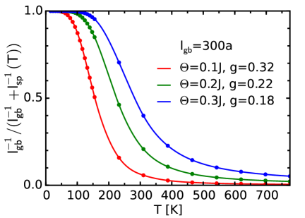
Figure 10: (Color online) Renormalization factor of the inverse mean-free path due to grain boundaries from spin-phonon scattering for various $\Theta_{D}$ and $g$, $J=1550$K (lines are guides to the eye).

IV.6.2 Grain boundaries and phonons

We now would like to test if the magnon-phonon scattering can have a significant impact on the magnon mean-free path and thermal conductivity. For that, we calculate numerically the spin-phonon current relaxation rate $(\mathbf{M}(i0^{+})/\bm{\chi})_{\mu\nu}=\delta_{\mu\nu}/\tau_{{\rm sp}}$ from (IV.2) as discussed above and neglecting anomalous scattering. Then the spin-phonon transport mean-free path is defined as $l_{sp}=v\tau_{{\rm sp}}$ and can be combined with the grain-boundary mean-free path $l_{{\rm gb}}$ to see the effect of the former. To make such a comparison, we also need to introduce a dimensionless spin-phonon coupling constant. In line with the discussion of the asymptotic limits in Sec. IV.4 above and in accord with the results of Appendix B, such a dimensionless coupling can be written as $g\!=\!4S\lambda/(J\sqrt{2m\Theta_{D}})$. The range of its typical values is discussed in Sec. III.6 and Appendix C and it is concluded that it may not exceed unity.Bramwell90

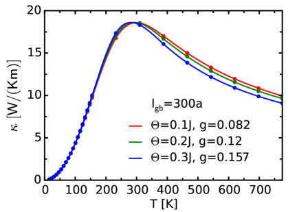
Figure 11: (Color online) Magnon thermal conductivity for the scattering by grain boundaries and phonons for various experimentally reasonable values of $\Theta_{D}$ and $g$, $J=1550$K (lines are guides to the eye).

Figure 10 displays the ratio of the inverse magnon mean-free paths with and without the spin-phonon scattering $l_{{\rm gb}}^{-1}/(l_{{\rm gb}}^{-1}+l_{{\rm sp}}^{-1}(T))$ for a range of resonable spin-phonon coupling constants and Debye temperatures. This Figure clearly demonstrates that phonons can be expected to be the dominant scatterers for $T\gtrsim 200K$ in large-$J$ antiferromagnets with a modest spin-phonon coupling.

In Figure 11 the thermal conductivity is shown for the scenario when only grain boundaries and phonons are involved in magnon scattering and for several representative sets of $\Theta_{D}$ and $g$. The latter are chosen to yield the same maximal value of $\kappa(T)$ at fixed $l_{{\rm gb}}$, with $J$ and other parameters fixed to loosely match La₂CuO₄. Hereafter all plots of the thermal conductivity display absolute values of $\kappa$. These follow from our calculations, scaling the 2D conductivity to the 3D material Hess03 , and using $l_{gb}Jk_{B}/(\hbar ac_{z})\simeq 645$W/(Km), for $J\simeq k_{B}1550$K and $l_{gb}\simeq 300a$, with intra(inter)-plane lattice constants $a$($c_{z}$) from Kastner98 . We emphasize, that the magnitude of $\kappa$ shown in Fig. 11 is within the typical range for La₂CuO₄. Hess03 ; others The Figure shows that the spin-phonon coupling constants necessary to effectively suppress the conductivity at $T\gtrsim\Theta_{D}$ are well within the acceptable values. Moreover, the Figure demonstrates that a rather natural temperature range for the maximum conductivity to occur in La₂CuO₄ and related materials is of the order of $\Theta_{D}$. Comparing with Fig. 9, one can see that the decrease of $\kappa$ vs $T$ occurs in the temperature regime where no well-defined power law exists for $\tau_{{\rm sp}}^{-1}(T)$, independently of the choice of the Debye energy.

Fig. 11 should also be compared with the upper curve in Fig. 6, which is obtained from the effective $1/\tau$-approximation within the Boltzmann formalism. Taking into account the differences between the $1/\tau$-approximation in Boltzmann approach and the memory function calculations, different types of modeling of the phonon bath, and keeping in mind differences in Debye energies and spin-phonon coupling constants, the close similarity of the overall shape and other features of the $\kappa(T)$ curves from the Boltzmann and the memory function approaches in Figs.  6 and 11 are remarkable.

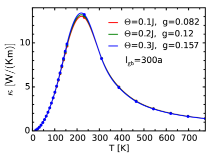
Figure 12: (Color online) Magnon thermal conductivity for the scattering off the effective grain boundary due to temperature-dependent correlation length and phonons for various experimentally reasonable values of $\Theta_{D}$ and $g$, $J=1550$K (lines are guides to the eye).

IV.6.3 Grain boundaries, phonons, and finite correlation length

Next we take into account scattering due to the finite spin-spin correlation length in the paramagnetic phase above the ordering Néel temperature, analogous to the discussion in Sec. III.7. Similar to the Boltzmann approach, a formally proper treatment of its effects is beyond the present study. A qualitative description, however, can be obtained readily. First, a finite correlation length implies a mass gap in the magnon dispersion, discussed in Sec. III.7, see Eq. (28).Takahashi Second, since the notion of magnetic order is meaningful only within patches of linear dimension $\sim\xi(T)$, Eq. (26), the system consists of effective “grains” with a temperature-dependent size $l_{gb}(T)\approx\mathrm{min}(l_{{\rm gb}},\xi(T))$, the sentiment expressed earlier in Sec. III. Once again, Matthiessen’s rule is used to yield a smooth crossover between the two grain-boundary regimes as a function of temperature and to include the spin-phonon scattering with the inverse mean-free path given by $l^{-1}(T)=l^{-1}_{gb}+\xi^{-1}(T)+l^{-1}_{sp}$.

First, recalculating $\kappa$ within the relaxation time approximation, Eq. (39), with a constant scattering time $\tau$ and the mass gap due to correlation-length in the magnon dispersion, Eq. (28), affects $\kappa$ only weakly and only at higher temperatures, in a broad agreement with the conclusions reached in Sec. III.8. For brevity, we will not study the impact of the mass gap on the memory function. In turn, the main effect of the correlation length on the thermal conductivity is from the limiting of the mean-free path by $\xi(T)$. For the parameters relevant to the cuprates, the correlation length gets short enough to likely dominate dominate the thermal conductivity for $T\gtrsim 250$K.

Our Figures 12 and 13 display the combined effect of spin-phonon and effective boundary scattering, discarding the magnon mass gap. Fig. 12 shows that at high temperatures, in contrast to the rather slow decrease of thermal conductivity in Fig. 11, $\kappa(T)$ is dominated by the exponential decrease of the effective grain size $\xi(T)$. This figure also shows that small differences in the results Fig. 11 due to differences in coupling constants and Debye energies are completely suppressed by inclusion of $\xi(T)$. Fig. 13 contrasts the various scattering mechanisms against each other. This figure clearly demonstrates that while the spin-spin correlation length seems to provide the major limit on $\kappa(T)$ at higher temperatures, magnon-phonon scattering still contributes significantly to the suppression of the magnon heat current up to high temperatures.

Once more we emphasize the close similarity of the combined results from the memory function method in Fig. 13 with those from the Boltzmann theory in Fig. 7. Given that these results have been obtained independently from two distinct theoretical approaches, this agreement strongly corroborates our main conclusions.

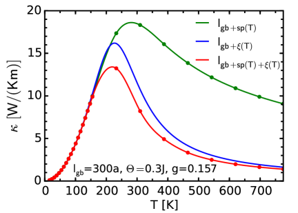
Figure 13: (Color online) Contrasting impact of different scattering mechanisms on the thermal conductivity. Phonons and crystalline grain boundary (upper curve), correlation length and crystalline grain boundary (middle curve), phonons, correlation length, and crystalline grain boundary (lower curve).

V Summary

To summarize, we have considered relaxation mechanisms of 2D magnons in large-$J$ antiferromagnets such as La₂CuO₄ with the goal of providing a basis for quantitative calculations of thermal transport by spin degrees of freedom in this class of materials. We conclude that the magnon thermal conductivity in these and related systems is limited by three key scattering mechanisms: grain boundaries, 2D correlation length, and magnon-phonon scattering, the latter being effective at intermediate and high temperatures, $T\!\gtrsim\!\Theta_{D}$. Impurity-like lattice-induced disorder and magnon Umklapp scattering have been found to be less important.

The bulk of our consideration has been devoted to the scattering of 2D magnons on 3D phonons, with acoustic and optical phonon branches examined in detail. Within the Boltzmann approach and $1/\tau$ approximation we have advocated the use of a simplified “effective” phonon DoS approach, which allows for straightforward yet fairly realistic calculations yielding an effective expression for the magnon relaxation rate on optical and acoustic phonons that contains minimal number of parameters. We have also employed the memory function approach, in which we have retained the full microscopic expressions for the magnon and phonon spectra, with the only approximation being the coupling of spins to only a single dispersive phonon branch.

Within both approaches, we have closely analyzed the power-law asymptotic regimes of the magnon relaxation rates involving acoustic and optical, or zone-boundary, phonons. Not only have such investigations proven very instructive in the analysis of which part of the magnon population is affected most strongly by phonons, but also have demonstrated a remarkable accord between the two very different theoretical approaches to the transport problem.

In both Boltzmann and memory functions approaches, we have demonstrated that having a modest spin-phonon coupling, well within a reasonable range of parameters, phonons can have a significant impact on the magnon mean-free path and thermal conductivity. Taking into account other scattering mechanisms within the thermal conductivity calculations, we have concluded that magnon thermal conductivity in large-$J$ antiferromagnets should be largely controlled by the “boundary-like” scatterings, coming from either the real grain boundaries or the 2D correlation length, with a substantial correction from the magnon-phonon scattering, affecting $\kappa(T)$ at intermediate and high temperatures, $T\!\gtrsim\!\Theta_{D}$. We have also demonstrated that the results of both approaches on thermal conductivity are remarkably similar.

Appendix A Spin model

For the spin system we consider the two-dimensional, nearest-neighbor, spin-1/2 Heisenberg antiferromagnet on a square-lattice

$${\cal H}_{\rm s}=J\sum_{\langle ij\rangle}{\bf S}_{i}\cdot{\bf S}_{j}\,,$$ (52)

where summation is over the nearest-neighbor bonds and $J$ is the exchange coupling constant. We treat this model using standard linear spin-wave theory. For the bipartite lattice we transform from the laboratory to the rotated frame for spins and bosonize spin operators according to

$$S^{z_{0}}_{i}=e^{i{\bf Q}{\bf r}_{i}}S^{z}_{i},\ \ S^{x_{0}}_{i}=e^{i{\bf Q}{\bf r}_{i}}S^{x}_{i},\ \ S^{y_{0}}_{i}=S^{y}_{i},\ \ \ \$$ (53)

$$S^{z}_{i}=S-b_{i}^{\dagger}b_{i},\ \ S_{i}^{+}=\left(S_{i}^{-}\right)^{\dagger}\approx b_{i}\sqrt{2S}\,,$$

where ${\bf Q}=(\pi,\pi)$ is the antiferromagnetic ordering vector. Then, within the $1/S$ approximation, one needs to retain only quadratic terms in the Hamiltonian (52)

$${\bf S}_{i}\cdot{\bf S}_{i+\delta}\Rightarrow S\Big{\{}b_{i}^{\dagger}b_{i}+b_{i+\delta}^{\dagger}b_{i+\delta}-b_{i+\delta}^{\dagger}b_{i}^{\dagger}-b_{i+\delta}b_{i}\Big{\}}.\ \$$ (54)

After the Fourier transform, the subsequent treatment of (52) involves Bogolyubov transformation of magnons given by

$$b_{\bf k}\!=\!u_{\bf k}\beta_{\bf k}\!+\!v_{\bf k}\beta^{\dagger}_{\bf-k}\,,$$ (55)

with

$$u_{\bf k}=\sqrt{\frac{1+\nu_{\bf k}}{2\nu_{\bf k}}},\ \ v_{\bf k}=sign\left(\gamma_{\bf k}\right)\sqrt{\frac{1-\nu_{\bf k}}{2\nu_{\bf k}}},$$ (56)

where $\nu_{\bf k}\!=\!\sqrt{1-\gamma_{\bf k}^{2}}$ is related to the magnon energy via $\varepsilon_{\bf k}\!=\!4JS\nu_{\bf k}$ and $\gamma_{\bf k}\!=\!\left(\cos k_{x}\!+\!\cos k_{y}\right)/2$. Finally, the spin-wave Hamiltonian is given by

$${\cal H}_{\rm s}^{(2)}=\sum_{\mathbf{k}}\varepsilon_{\mathbf{k}}\beta_{\mathbf{k}}^{\dagger}\beta_{\mathbf{k}}^{\vphantom{\dagger}}\,,$$ (57)

At long wavelength $\varepsilon_{\mathbf{k}}\approx vk$ with the spin-wave velocity $v=\sqrt{2}J$.

Appendix B Microscopic derivation of spin-phonon Hamiltonians: vertices, polarizations, etc.

B.0.1 Spin-phonon Hamiltonian: Bravias lattice

For an isotropic, nearest-neighbor interaction of spins and considering the lattice of only magnetic ions, the most natural source of the spin-phonon coupling is from the modifications of the superexchange due to local stretching or compression of the bond lengthDixon

$${\cal H}_{\rm s-ph}=\sum_{\langle ij\rangle}\delta J\left({\bf r}_{j}-{\bf r}_{i}\right){\bf S}_{i}\cdot{\bf S}_{j}$$ (58)

$$\phantom{{\cal H}_{\rm s-ph}}\approx\frac{\lambda}{2}\sum_{i,\delta}\left(\mbox{\boldmath$\delta$}\cdot\Delta{\bf U}_{i,\delta}\right){\bf S}_{i}\cdot{\bf S}_{i+\delta}\,,$$

where $\lambda\!=\!a\partial J/\partial r$, with $a$ being the lattice constant, $\delta$ runs over the nearest neighbors, $\delta$ are the corresponding unit vectors of the lattice, $\Delta{\bf U}_{i,\delta}\!\equiv\!\left({\bf U}_{i+\delta}\!-\!{\bf U}_{i}\right)$, and ${\bf U}_{i}$ is the displacement vector of the $i$th ion. While the Hamiltonian in (58) is rather general, one can see it as describing a single 2D plane of spins on a square lattice, representative of a CuO₂ plane of La₂CuO₄. Below, we will extend this picture to a tetragonal array of magnetically decoupled planes to take into account the 3D nature of phonons. Note that while the displacement of ions are described by 3D vectors, in (58) only their projections on the in-plane bonds ($\delta$) matter.

After bosonizing spin operators according to (54), using the symmetry of the square lattice, Fourier transform, and some algebra, we obtain

$${\cal H}_{\rm s-ph}=4i\lambda S\sum_{\bf q,k,k^{\prime}}\sum_{\mbox{\boldmath$\delta$}}\left(\mbox{\boldmath$\delta$}\cdot{\bf U}_{\bf q}\right)\sin\left(\frac{{\bf k}-{\bf k^{\prime}}}{2}{\mbox{\boldmath$\delta$}}\right)$$

$$\phantom{{\cal H}=4i\lambda S}\bigg{\{}\cos\left(\frac{{\bf k}-{\bf k^{\prime}}}{2}{\mbox{\boldmath$\delta$}}\right)b_{\bf k^{\prime}}^{\dagger}b_{\bf k}$$ (59)

$$\phantom{{\cal H}=4i\lambda S}-\frac{1}{2}\cos\left(\frac{{\bf k}+{\bf k^{\prime}}}{2}{\mbox{\boldmath$\delta$}}\right)\left(b_{\bf k^{\prime}}^{\dagger}b_{-\bf k}^{\dagger}+b_{-\bf k^{\prime}}b_{\bf k}\right)\bigg{\}}\,,$$

where ${\bf q}\!=\!({\bf k}-{\bf k^{\prime}},q_{\perp})$ and the summation over the directions of the bond now takes the values of only two unit vectors, $\mbox{\boldmath$\delta$}\!=\!{\bf\hat{x}}$ and ${\bf\hat{y}}$. In derivation of (59) we have performed summation over the sites of the tetragonal lattice of magnetically decoupled planes. It is natural that the in-plane component of the phonon momentum (in the index of ${\bf U}_{\bf q}$) is tied to the magnon momenta via momentum conservation, ${\bf q}_{\parallel}\!=\!{\bf k}-{\bf k^{\prime}}$, while the component of the phonon momentum perpendicular to the plane, ${\bf q}_{\perp}$, is not conserved and is an independent variable in the sum in (59). This is because the 2D magnons have zero coupling between the planes (infinite mass in that direction) and thus provide no restriction on ${\bf q}_{\perp}$.

The subsequent treatment of (59) involves Bogolyubov transformation of magnons as in (55) and rewriting the displacement operators in terms of phonons. For the Bravias lattice, the ${\bf q}$’s Fourier component of the lattice displacement is given by

$${\bf U}_{\bf q}=\sum_{\ell}\frac{\mbox{\boldmath$\xi$}^{\ell}_{\bf q}}{\sqrt{2m\omega^{\ell}_{\bf q}}}\left(a^{\dagger}_{{\bf q}\ell}+a_{-{\bf q}\ell}\right),$$ (60)

where $\ell=1,2,3$ numerates one longitudinal and two transverse phonon polarizations, $\xi$${}^{\ell}_{\bf q}$ are the polarization unit vectors, $m$ is the mass of the unit cell, and $\omega^{\ell}_{\bf q}$ and $a_{{\bf q}\ell}$ are the energies and operators of the corresponding phonon branches, respectively.

Applying (60) and (56) to (59) we obtain

$${\cal H}_{\rm s-ph}=\sum_{{\bf k,k^{\prime}},q_{\perp}}\sum_{\ell}\Big{\{}V^{\ell}_{\bf k,k^{\prime},q}\beta_{\bf k^{\prime}}^{\dagger}\beta_{\bf k}$$ (61)

$$\phantom{{\cal H}=}+\frac{1}{2}\,V^{{\rm od},\ell}_{\bf k,k^{\prime},q}\left(\beta_{\bf k^{\prime}}^{\dagger}\beta_{-\bf k}^{\dagger}+\mbox{H.c.}\right)\Big{\}}\left(a^{\dagger}_{{\bf q}\ell}+a_{-{\bf q}\ell}\right),$$

where “normal” and “anomalous” magnon-phonon vertices are

$$V^{\ell}_{\bf k,k^{\prime},q}=\frac{4S\lambda}{\sqrt{2m\omega^{\ell}_{\bf q}}}\sum_{\alpha=x,y}\xi^{\ell,\alpha}_{\bf q}\sin\frac{q_{-}^{\alpha}}{2}$$ (62)

$$\phantom{V^{\ell}_{\bf k,k^{\prime},q}}\times\Big{\{}\cos\frac{q_{-}^{\alpha}}{2}\left(uu^{\prime}+vv^{\prime}\right)-\cos\frac{q_{+}^{\alpha}}{2}\left(uv^{\prime}+vu^{\prime}\right)\Big{\}},$$

$$V^{{\rm od},\ell}_{\bf k,k^{\prime},q}=\frac{4S\lambda}{\sqrt{2m\omega^{\ell}_{\bf q}}}\sum_{\alpha=x,y}\xi^{\ell,\alpha}_{\bf q}\sin\frac{q_{-}^{\alpha}}{2}$$ (63)

$$\phantom{V^{{\rm od},\ell}_{\bf k,k^{\prime},q}}\times\Big{\{}\cos\frac{q_{-}^{\alpha}}{2}\left(uv^{\prime}+vu^{\prime}\right)-\cos\frac{q_{+}^{\alpha}}{2}\left(uu^{\prime}+vv^{\prime}\right)\Big{\}},$$

where we have absorbed $i$ in the definition of phonon operators, $\xi^{\alpha}$ and $q_{\pm}^{\alpha}$ are the $x$ and $y$ projections of the corresponding vectors, and we have introduced shorthand notations ${\bf q}_{\pm}\!=\!{\bf k}\!\pm\!{\bf k^{\prime}}$, $u^{(\prime)}\!=\!u_{\bf k^{(\prime)}}$, and $v^{(\prime)}\!=\!v_{\bf k^{(\prime)}}$.

B.0.2 Asymptotics and polarizations

Of interest, of course, is the asymptotic behavior of these vertices in the vicinity of ${\bf k},{\bf k^{\prime}}\!\rightarrow\!\mbox{\boldmath$\Gamma$},{\bf Q}$ as the momenta of magnons are confined to these regions at not too high temperatures.

Expanding (62) for magnon momenta ${\bf k},{\bf k^{\prime}}\!\rightarrow\!\mbox{\boldmath$\Gamma$}$ (or ${\bf Q}$), which also corresponds to ${\bf q}_{\parallel}\!\rightarrow\!0$, gives $\alpha=x,y$ components of the vertex

$$V^{\ell,\alpha}_{\bf k,k^{\prime},q}\approx\frac{S\lambda\,\xi^{\ell,\alpha}_{\bf q}}{\sqrt{4m\omega^{\ell}_{\bf q}}}\ q^{\alpha}_{\parallel}\sqrt{|{\bf k}||{\bf k^{\prime}}|}\,\left(1+\frac{2k^{\alpha}k^{\prime\alpha}}{|{\bf k}||{\bf k^{\prime}}|}\right),$$ (64)

and expansion of (63) yields $V^{{\rm od},\ell,\alpha}_{\bf k,k^{\prime},q}=-V^{\ell,\alpha}_{\bf k,k^{\prime},q}$.

In general, three polarization vectors $\xi$${}^{\ell}_{\bf q}$ in (60) should be obtained as solutions of the dynamical matrix equation for the lattice vibrations of the tetragonal Bravias lattice for each ${\bf q}$-vector. However, in the long-wavelength limit ${\bf q}\!\rightarrow\!0$, these solutions can be classified as in the continuum as one longitudinal and two transverse modes. For the former, $\xi$${}^{(3)}_{\bf q}\!\approx\!{\bf q}/|{\bf q}|$ is along the momentum of the phonon, while the latter can be chosen freely as an orthogonal pair in the plane perpendicular to ${\bf q}$. For instance, a convenient choice is $\xi$${}^{(1)}_{\bf q}\!\approx\!{\bf y}\times{\bf q}/|{\bf y}\times{\bf q}|$, which ensures that it is orthogonal to the $y-q$ plane. Since in (62)–(64) we are interested only in $x$ and $y$ projections of the polarization vectors, this choice leaves nonzero only $\xi^{(1),x}_{\bf q}$ component.

However, the situation is even simpler because, according to the discussion in Sec. III.2, in a typical scattering process component of the phonon momentum perpendicular to the plane is much larger than the in-plane component, $|{\bf q}_{\perp}|\!\gg\!|{\bf q}_{\parallel}|$. This means that the in-plane projections of the longitudinal phonon polarization vector are negligible, $\xi^{(3),x(y)}_{\bf q}\!\approx\!q_{\parallel}^{x(y)}/q_{\perp}\!\ll\!1$. In turn, this means that the polarizations of the two transverse modes lie almost entirely in the $x-y$ plane and the corresponding vectors can simply be chosen along the $x$ and $y$ axes with $\xi^{(1),x}_{\bf q}\!\approx\!\xi^{(2),y}_{\bf q}\!\approx\!1$ and $\xi^{(1),y}_{\bf q}\!\approx\!\xi^{(2),x}_{\bf q}\!\approx\!0$. Therefore, it is the transverse phonons with the momentum largely orthogonal to the antiferromagnetic planes that couple most strongly to the spin excitations. As a result, summation over $\ell$ in (61) should concern only them. We note that the same arguments have been used previously for the spin-phonon coupling in 1D spin chains, see Ref. RC, .

Thus, using $\omega^{(1)}_{\bf q}\!\approx\!\omega^{(2)}_{\bf q}\!\approx\!c|{\bf q}|$ for the transverse branches, the magnon-phonon coupling with the acoustic phonons is reduced to just two non-zero terms

$$V^{(1),x}_{\bf k,k^{\prime},q}\approx g_{\rm sp}^{\rm ac}\,\frac{q^{x}_{\parallel}}{\sqrt{|{\bf q}|}}\,\sqrt{|{\bf k}||{\bf k^{\prime}}|}\,\left(1+\frac{2k^{x}k^{\prime x}}{|{\bf k}||{\bf k^{\prime}}|}\right),\ \ \$$ (65)

$$V^{(2),y}_{\bf k,k^{\prime},q}\approx g_{\rm sp}^{\rm ac}\,\frac{q^{y}_{\parallel}}{\sqrt{|{\bf q}|}}\,\sqrt{|{\bf k}||{\bf k^{\prime}}|}\,\left(1+\frac{2k^{y}k^{\prime y}}{|{\bf k}||{\bf k^{\prime}}|}\right),$$

where $g_{\rm sp}^{\rm ac}\!=\!S\lambda/2\sqrt{mc}$ and the results are the same for the anomalous coupling $V^{{\rm od},\ell,\alpha}_{\bf k,k^{\prime},q}$.

Since the vertices in (65) couple to different but degenerate phonon branches, they will contribute independently to the scattering probability, so that $|V_{\rm tot}|^{2}\!=\!|V^{(1),x}|^{2}\!+\!|V^{(2),y}|^{2}$. Then it is natural to introduce an effective coupling to just one phonon branch that would lead to the same scattering rate

$$V^{\rm eff}_{\bf k,k^{\prime},q}\approx g_{\rm sp}^{\rm ac}\,\frac{|{\bf q}_{\parallel}|}{\sqrt{|{\bf q}|}}\,\sqrt{|{\bf k}||{\bf k^{\prime}}|}\,,$$ (66)

in which we simply ignored the angular dependence in the brackets in (65) [second terms]. This is equivalent only to a quantitative (order of 1) change in the effective coupling constant. Needless to say, the result in (66) is identical to the coupling proposed in (8) and used throughout the paper.

With that the effective Hamiltonian for magnon-phonon coupling becomes

$${\cal H}^{\rm eff}_{\rm s-ph}=\sum_{{\bf k,k^{\prime}},q_{\perp}}V^{\rm eff}_{\bf k,k^{\prime},q}\Big{\{}\beta_{\bf k^{\prime}}^{\dagger}\beta_{\bf k}+\frac{1}{2}\left(\beta_{\bf k^{\prime}}^{\dagger}\beta_{-\bf k}^{\dagger}+\mbox{H.c.}\right)\Big{\}}$$

$$\phantom{{\cal H}_{\rm eff}=\sum_{{\bf k,k^{\prime}},q_{\perp}}V^{\rm eff}_{\bf k,k^{\prime},q}}\times\left(a^{\dagger}_{{\bf q}\ell}+a_{-{\bf q}\ell}\right),$$ (67)

B.0.3 Zone-boundary phonon

A yet another asymptotic consideration is relevant for the magnon-phonon coupling on a Bravias lattice. It concerns scattering of a magnon between two branches, from the vicinity of $\Gamma$ point to the gapless branch at the antiferromagnetic ordering vector ${\bf Q}$ or vice versa. Therefore, of interest are the limits ${\bf k}\!\rightarrow\!\mbox{\boldmath$\Gamma$}$ and ${\bf k^{\prime}}\!\rightarrow\!{\bf Q}$ for vertices in (62) and (63). Importantly, the phonon involved in such a process has a large momentum with the in-plane component ${\bf q}_{\parallel}\!\approx\!-{\bf Q}$, which corresponds to a zone-boundary excitation with the energy of order $\Theta_{\rm D}$ and is similar to the optical modes considered next.

Expansion of the “magnon part” [content of the curly brackets] in (62) and (63) gives

$$V^{\ell}_{\bf k,k^{\prime},q}=\frac{4S\lambda}{\sqrt{2m\omega^{\ell}_{\bf q}}}\sum_{\alpha}\xi^{\ell,\alpha}_{\bf q}\bigg{\{}\frac{k^{\prime\alpha}|{\bf k}|-k^{\alpha}|{\bf k^{\prime}}|}{2\sqrt{|{\bf k}||{\bf k^{\prime}}|}}\bigg{\}},\ \ \ \ \ \ \$$ (68)

$$V^{{\rm od},\ell}_{\bf k,k^{\prime},q}=\frac{4S\lambda}{\sqrt{2m\omega^{\ell}_{\bf q}}}\sum_{\alpha}\xi^{\ell,\alpha}_{\bf q}\bigg{\{}\frac{k^{\alpha}|{\bf k^{\prime}}|+k^{\prime\alpha}|{\bf k}|}{2\sqrt{|{\bf k}||{\bf k^{\prime}}|}}\bigg{\}},$$

where we have shifted ${\bf k^{\prime}}\!\rightarrow\!{\bf Q}\!+\!{\bf k^{\prime}}$ and also used that $\sin(q^{\alpha}_{\parallel}/2)\!\approx\!-1$ for ${\bf q}_{\parallel}\!\approx\!-{\bf Q}$. Focusing now on the “normal” vertex and following the same choice of polarization vectors as above leads to two non-zero vertices

$$V^{(1),x}_{\bf k,k^{\prime},q}\approx g_{\rm sp}^{\rm zb}\,\frac{k^{\prime x}|{\bf k}|-k^{x}|{\bf k^{\prime}}|}{2\sqrt{|{\bf k}||{\bf k^{\prime}}|}}\,,$$ (69)

$$V^{(2),y}_{\bf k,k^{\prime},q}\approx g_{\rm sp}^{\rm zb}\,\frac{k^{\prime y}|{\bf k}|-k^{y}|{\bf k^{\prime}}|}{2\sqrt{|{\bf k}||{\bf k^{\prime}}|}}\,,$$

with the coupling constant to the zone-boundary phonon $g_{\rm sp}^{\rm zb}\!=\!4S\lambda/\sqrt{2m\Theta_{\rm D}}$. Combining the two couplings to different phonon branches into one effective vertex gives

$$V^{\rm eff}_{\bf k,k^{\prime},q}\approx g_{\rm sp}^{\rm zb}\,\sqrt{|{\bf k}||{\bf k^{\prime}}|}\,\sin(\varphi/2),$$ (70)

where $\varphi$ is the angle between ${\bf k}$ and ${\bf k^{\prime}}$ and anomalous vertex is the same with $\sin\!\rightarrow\!\cos$. The only difference of the effective coupling in (70) from the coupling to the optical phonon proposed in (7) is the additional angular dependence. It is easy to see that when calculating the scattering probabilities with $|V|^{2}$ the latter will be averaged to an additional factor $1/2$ and thus corresponds to a simple change of the effective coupling constant.

B.0.4 Optical phonons

To introduce optical phonons into the spin-lattice coupling model one needs to depart from the Bravias picture of (58). For that, keeping in mind cuprates, mutual displacement of copper ions $\Delta{\bf U}_{i,\delta}\!\equiv\!\left({\bf U}_{i+\delta}\!-\!{\bf U}_{i}\right)$ should now be recognized as involving the complete set of phonon normal modes. That is, the summation over $\ell$ in (60) should now be treated as involving not only three acoustic branches of the Bravias lattice, but the entire group of optical modes as well. In that sense, the general form of the spin-coupling Hamiltonian in (59) and the entire consideration of it remains valid with the magnon-phonon coupling constants and optical phonon energies used accordingly.

It is then clear that the small-${\bf q}_{\parallel}$ scatterings involving optical branches should be less important than the ones involving acoustic modes, while the large-${\bf q}_{\parallel}$ do not carry additional smallness of $|{\bf q}_{\parallel}|\!\sim\!T/v$ and should be important. Therefore, a consideration of the leading effect of the optical-phonon coupling is very similar to that of the zone-boundary phonon above. Thus, without going into consideration of the details of the crystal structure of specific materials and neglecting nonessential angular dependence similarly to the cases considered above yields

$$V^{\rm eff}_{\bf k,k^{\prime},q}\approx g_{\rm sp}^{\rm opt}\,\sqrt{|{\bf k}||{\bf k^{\prime}}|}\,,$$ (71)

with $g_{\rm sp}^{\rm opt}\!\approx\!4\lambda S/\sqrt{2m\omega_{0}}$ where $\omega_{0}$ is the energy of the optical branch. Thus, the form of the magnon-phonon interaction proposed in (7) is verified. While, obviously, the coupling strength must depend on the type of the optical model involved, one can suggestRonnow14 the so-called “stretching mode” at high energies as a strong candidate for a significant spin-phonon coupling.

Appendix C Magnitude of spin phonon coupling

All three effective magnon-phonon coupling constants, to acoustic, to zone-boundary, and to optical modes, introduced in Eqs. (65), (69), and (71), respectively, have very similar structure: $g_{\rm sp}\!\propto\!\lambda/\sqrt{2m\Theta_{D}}$ with a coefficient of order of unity. Here $\lambda\!=\!a\partial J/\partial r\!\approx\!\gamma J$ is the response of the superexchange constant to the atomic displacement. It has been arguedBramwell90 that because the superexchange is very sensitive to the interatomic distance, the typical values of $\gamma$ are $\sim\!10-20$. However, this largeness is offset by the smallness of a characteristic scale associated with phonons,Bramwell90 $1/\sqrt{m\Theta_{D}}\!\sim\!1/100$. This is, actually, the same parameter that characterizes the smallness of the typical magnitude of the zero-point atomic displacement relative to the interatomic distanceZiman or the smallness of the typical velocity of an atom in a lattice relative to the sound velocity. Thus, the physical range of the magnon-phonon constants is $g_{\rm sp}/J\!\sim\!0.1$.

To make a closer estimate of the spin-phonon coupling constants as related to the cuprates, we use $m=m_{\rm Cu}$ and a typical phonon Debye energy $\Theta_{D}=400$K. The largest uncertainty is in the value of $\partial J/\partial r=\gamma J/a$ with $\gamma\simeq O(3\ldots 14)$ Ronnow14 ; Takigawa . Therefore

$$\frac{4S\lambda\hbar}{\sqrt{2ma^{2}k_{B}\Theta_{D}}}\equiv gJ\sim O(0.05\dots 0.3)\,J\,,$$ (72)

where we have used $a\simeq 3.8\mathbf{\textrm{\AA}}$, as in La₂CuO₄. This defines the dimensionless spin-phonon coupling constant $g$ and demonstrates that spin-phonon coupling in the cuprates, while significant, is still within the bounds to justify the use of perturbation theory.

Appendix D Verification of the “effective phonon DoS” approach

Here we complement the discussion of Secs. III.4 and III.5 by providing more verifications of the effective DoS approach advocated in this work.

D.0.1 Optical phonons

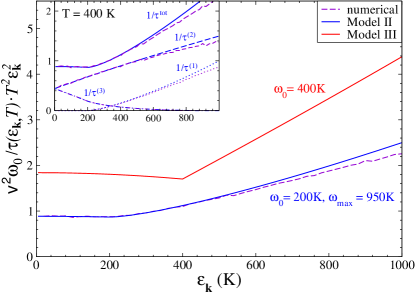
Figure 14: (Color online) Magnon relaxation rate on the optical phonons, Eq. (16), vs $\varepsilon_{\bf k}$ for a representative $T\!=\!400$K and for effective phonon DoS Models II and III in Eqs. (13) and (14). The results are normalized to the high-temperature asymptotic behavior of the phonon-absorption term $\tau_{\bf k}^{(2)}$, Eq. (17), [$T^{2}\varepsilon_{\bf k}^{2}/v^{2}\omega_{0}$]. Parameters are indicated in the graph. The vertical axis is in units of $(g_{\rm sp}^{\rm opt}/v)^{2}$. Dashed line is the result of the direct numerical integration in Eq. (5) for the dispersive optical phonon in Fig. 2 without the approximation of Eq. (10). Inset shows individual contributions of the three diagrams in Fig. 1 for both the effective DoS approach (16) with the Model II and the direct numerical integration.

For the “Model III” in Eq. (14) (flat phonon mode) of the effective phonon DoS the integral in Eq. (16) is trivially removed and the relaxation rate is given by a compact analytical expression

$$\frac{1}{\tau_{\bf k}}\approx\left(\frac{g_{\rm sp}^{\rm opt}}{v}\right)^{2}\left(\frac{\varepsilon_{\bf k}}{v^{2}}\right)$$ (73)

$$\times\Big{\{}\Theta\big{(}\varepsilon_{\bf k}-\omega_{0}\big{)}\left(\varepsilon_{\bf k}-\omega_{0}\right)^{2}\Big{(}n(\omega_{0})+n(\varepsilon_{\bf k}-\omega_{0})+1\Big{)}$$

$$\phantom{\frac{1}{\tau_{\bf k}}\Big{\{}\Theta\big{(}\varepsilon_{\bf k}-\omega_{0}\big{)}}+\left(\varepsilon_{\bf k}+\omega_{0}\right)^{2}\Big{(}n(\omega_{0})-n(\varepsilon_{\bf k}+\omega_{0})\Big{)}$$

$$\phantom{\frac{1}{\tau_{\bf k}}\Big{\{}}+\Theta\big{(}\omega_{0}-\varepsilon_{\bf k}\big{)}\left(\omega_{0}-\varepsilon_{\bf k}\right)^{2}\Big{(}n(\omega_{0}-\varepsilon_{\bf k})-n(\omega_{0})\Big{)}\Big{\}}.$$

An identical expression can be obtained directly from Eq. (5) for the optical phonon energy $\omega_{\bf q}\!=\!\omega_{0}$ and linearized magnon energy and magnon-phonon vertex in (6) and (7). Thus, in this case, the effective phonon DoS approach is exact.

Fig. 4 shows the expected activated and high-temperature asymptotic behavior of the scattering rate vs $T$ from (18). Fig. 14 demonstrates the validity of another aspect of the asymptotic consideration in Eq. (17): the dependence of $1/\tau_{\bf k}$ on $\varepsilon_{\bf k}$ at $T\!>\!\omega_{0}$. The results in Fig. 14 are normalized to the high-temperature asymptotic behavior of the phonon-absorption term $1/\tau_{\bf k}^{(2)}$ in Eq. (17), $T^{2}\varepsilon_{\bf k}^{2}/v^{2}\omega_{0}$. Clearly, for $\varepsilon_{\bf k}\!<\!T$ such a behavior is confirmed (finite intersect of the vertical axis), while the phonon-emission term, $1/\tau_{\bf k}^{(1)}$, carries higher power of $\varepsilon_{\bf k}$, also in agreement with Eq. (17). In addition, the results of a direct 3D numerical integration in Eq. (5) for the dispersive optical phonon in Fig. 2, $\omega_{\bf q}\!\approx\!\omega_{0}\!+\!\alpha{\bf q}^{2}$, without the approximation of Eq. (10) are shown by the dashed line. Inset shows individual contributions of three diagrams in Fig. 1 for both the effective DoS approach (16) with the Model II and the direct numerical integration. One can see a very close agreement of the effective DoS method with the direct numerical integration in (5), which is achieved at a fraction of numerical cost as the former approach requires only a 1D integration in Eq. (16).

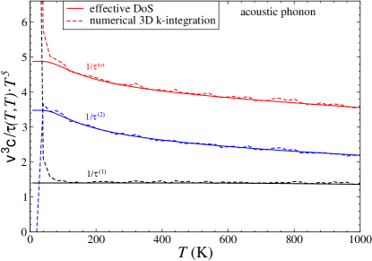
Figure 15: (Color online) $T$-dependence of the magnon relaxation rate on the acoustic phonons, Eq. (21), for $\varepsilon_{\bf k}\!=\!T$ and using effective phonon DoS model in Eq. (15). The results are normalized to the asymptotic behavior, Eq. (19), [$T^{5}/v^{3}\omega_{0}$]. Parameters are as discussed in text, Debye energy $\Theta_{D}\!=\!400$K. The vertical axis is in units of $(g_{\rm sp}^{\rm ac}/v)^{2}$. Individual contributions of the first two terms in (21) [diagrams in Fig. 1(a) and (b)] are indicated. Dashed lines are the result of the direct numerical 3D integration in Eq. (5) for the acoustic phonon without the approximation of Eq. (10).

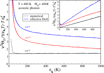
Figure 16: (Color online) Magnon relaxation rate, Eq. (21), vs $\varepsilon_{\bf k}$ for a representative $T\!=\!400$K and for effective phonon DoS model in Eq. (15). The results are normalized to the asymptotic behavior, Eq. (22), [$T\varepsilon_{\bf k}^{4}/v^{3}\Theta_{D}$]. Inset: Same with the normalization by $T^{2}\varepsilon_{\bf k}^{3}/v^{3}\Theta_{D}$.

D.0.2 Acoustic phonons

With the help of our Figs. 15 and 16 we provide a demonstration of the accuracy and numerical efficiency of the effective phonon DoS approach. In them the $T$- and $\varepsilon_{\bf k}$-dependencies of the relaxation rate by acoustic phonons from (21) are compared with an explicit numerical 3D integration in (5) with the magnon-phonon vertex from (8) and without the use of approximation (10). These figures also offer an additional confirmation of the asymptotic trends of Eqs. (19) and (22).

In Fig. 15, the $T$-dependence is shown for the relaxation rate Eq. (21) for $\varepsilon_{\bf k}\!=\!T$, i.e., on “thermal shell”. The results are normalized to $T^{5}/v^{3}\Theta_{D}$ to make the asymptotic behavior of (19) apparent. The vertical axis is in units of $(g_{\rm sp}^{\rm ac}/v)^{2}$. We also show individual contributions of the first two terms in (21), while the third is negligible as discussed above. The results of a direct 3D numerical integration in Eq. (5) for acoustic phonon (within the Debye approximation) without the approximation of Eq. (10) are shown by dashed lines. One can see a very close quantitative agreement of the effective DoS method with the direct numerical integration. At very low $T$, the direct numerical procedure becomes unreliable due to very small ${\bf k^{\prime}}$- and ${\bf q}$-space of integration relevant for the scattering. Again, the high-accuracy results of the effective DoS approach are achieved at a fraction of the numerical cost of the direct integration.

Fig. 16 shows the dependence of $1/\tau_{\bf k}$ on $\varepsilon_{\bf k}$ at a representative $T\!=\!400$K. The results in Fig. 16 are normalized to the asymptotic behavior in Eq. (22), $T\varepsilon_{\bf k}^{4}/v^{3}\Theta_{D}$. Clearly, for $1/\tau^{(1)}$ such an asymptote is essentially precise for all the energies, while for the phonon-absorption term substantial deviations occur at lower energies, the feature also emphasized in the inset of Fig. 16. This can be analyzed by a more careful asymptotic treatment of Eq. (21) in the $\varepsilon_{\bf k}\!\ll\!T$ regime, which show that the smallness of the subleading terms by $c/v$ gets compensated by the largeness of $T/\varepsilon_{\bf k}$ for small enough $\varepsilon_{\bf k}$, and the ultimate asymptotic behavior of this term in the $\varepsilon_{\bf k}\!\ll\!T$ regime is $1/\tau^{(2)}\!\sim\!T^{3}\varepsilon_{\bf k}^{2}/v^{4}$. As in Fig. 15, Fig. 16 shows a very close quantitative agreement of the effective DoS method with the direct numerical integration.

References

- (1) M. A. Kastner, R. J. Birgeneau, G. Shirane, and Y. Endoh, Rev. Mod. Phys. 70, 897 (1998).
- (2) D. J. Scalapino, Rev. Mod. Phys. 84, 1383 (2012).
- (3) K. Fujita, C. K. Kim, I. Lee, J. Lee, M. H. Hamidian, I. A. Firmo, S. Mukhopadhyay, H. Eisaki, S. Uchida, M. J. Lawler, E.-A. Kim, and J. C. Davis, Science 344, 612 (2014).
- (4) M. Vojta, Adv. Phys. 58, 699 (2009).
- (5) D. N. Basov, R. D. Averitt, D. van der Marel, M. Dressel, and K. Haule, Rev. Mod. Phys. 83, 471 (2011).
- (6) N. P. Armitage, P. Fournier, and R. L. Greene, Rev. Mod. Phys. 82, 2421 (2010).
- (7) B. Dalla Piazza, M. Mourigal, N. B. Christensen, G. J. Nilsen, P. Tregenna-Piggott, T. G. Perring, M. Enderle, D. F. McMorrow, D. A. Ivanov, and H. M. Rønnow, Nat. Phys. 11, 62 (2015).
- (8) O. P. Vajk, P. K. Mang, M. Greven, P. M. Gehring, and J. W. Lynn, Science 295, 1691 (2002).
- (9) C. Hess, B. Büchner, U. Ammerahl, L. Colonescu, F. Heidrich-Meisner, W. Brenig, and A. Revcolevschi, Phys. Rev. Lett. 90, 197002 (2003).
- (10) Y. Nakamura, S. Uchida, T. Kimura, N. Motohira, K. Kishio, K. Kitazawa, T. Arima, and Y. Tokura, Physica C: Superconductivity 185-189, 1409 (1991); M. Hofmann, T. Lorenz, K. Berggold, M. Grüninger, A. Freimuth, G. S. Uhrig, and E. Brück, Phys. Rev. B 67, 184502 (2003); X. F. Sun, J. Takeya, S. Komiya, and Y. Ando, Phys. Rev. B 67, 104503 (2003); J.-Q. Yan, J.-S. Zhou, and J. B. Goodenough, Phys. Rev. B 68, 104520 (2003).
- (11) C. Hess, etal., (unpublished).
- (12) Yu. A. Kosevich and A. V. Chubukov, Zh. Eksp. Teor. Fiz. 91, 1105 (1986) [Sov. Phys. JETP 64, 654 (1986)]; S. Ty̌c and B. I. Halperin, Phys. Rev. B 42, 2096 (1990); P. Kopietz, Phys. Rev. B 41, 9228 (1990).
- (13) P. S. Häfliger, S. Gerber, R. Pramod, V. I. Schnells, B. dalla Piazza, R. Chati, V. Pomjakushin, K. Conder, E. Pomjakushina, L. Le Dreau, N. B. Christensen, O. F. Syljuåsen, B. Normand, and H. M. Rønnow, Phys. Rev. B 89, 085113 (2014).
- (14) M. Takahashi, Phys. Rev. B 40, 2494 (1989).
- (15) L. Pintschovius, N. Pyka, W. Reichardt, A. Yu. Rumiantsev, N. L. Mitrofanov, A. S. Ivanov, G. Collin, and P. Bourges, Physica B 174, 323 (1991).
- (16) S. Bramwell, J. Phys. Condens. Matter 2, 7257 (1990).
- (17) A. L. Chernyshev and A. V. Rozhkov, Phys. Rev. B 72, 104423 (2005); A. V. Rozhkov and A. L. Chernyshev, Phys. Rev. Lett. 94, 087201 (2005).
- (18) C. Herring, Phys. Rev. 95, 954 (1954).
- (19) In practice, the “pseudo”-step-function can be chosen as , where and defines the “width” of the exponential turn-on for the scattering on the th optical mode.
- (20) B. I. Halperin and P. C. Hohenberg, Phys. Rev. Lett. 19, 700 (1967); Phys. Rev. 177, 952 (1969).
- (21) S. Chakravarty, B. I. Halperin, and D. R. Nelson, Phys. Rev. B 39, 2344 (1989).
- (22) S. Ty̌c, B. I. Halperin, and S. Chakravarty, Phys. Rev. Lett. 62, 835 (1989).
- (23) D. R. Grempel, Phys. Rev. Lett. 61, 1041 (1988).
- (24) A. M. Toader, J. P. Goff, M. Roger, N. Shannon, J. R. Stewart, and M. Enderle, Phys. Rev. Lett. 94, 197202 (2005).
- (25) H. M. Rønnow, D. F. McMorrow, R. Coldea, A. Harrison, I. D. Youngson, T. G. Perring, G. Aeppli, O. Syljuåsen, K. Lefmann, and C. Rischel, Phys. Rev. Lett. 87, 037202 (2001); 89, 079702 (2002); P. Kopietz and I. Spremo, Phys. Rev. Lett. 89, 079701 (2002).
- (26) M. Makivič and M. Jarrell, Phys. Rev. Lett. 68, 1770 (1992).
- (27) Hasenfratz, Eur. Phys. J. B 13, 11 (2000).
- (28) J. M. Ziman, Principles of the Theory of Solids, (Cambridge University Press, Cambridge, 1972).
- (29) S. P. Bayrakci, B. Keimer, and D. A. Tennant, ArXiv e-prints (2013), arXiv:1302.6476 [cond-mat.str-el].
- (30) P. Sengupta, A. W. Sandvik, and R. R. P. Singh, Phys. Rev. B 68, 094423 (2003).
- (31) D. Forster, Hydrodynamic Fluctuations, Broken Symmetry, and Correlation Functions (Benjamin, New York, 1975).
- (32) G. S. Dixon, Phys. Rev. B 21, 2851 (1980).
- (33) M. Takigawa, O. A. Starykh, A. W. Sandvik, and R. R. P. Singh, Phys. Rev. B 56, 13681 (1997).