Abstract

We construct a class of codimension-2 solutions in supergravity that realize T-folds with arbitrary $O(2,2,\mathbb{Z})$ monodromy and we develop a geometric point of view in which the monodromy is identified with a product of Dehn twists of an auxiliary surface $\Sigma$ fibered on a base $\mathcal{B}$. These defects, that we call T-fects, are identified by the monodromy of the mapping torus obtained by fibering $\Sigma$ over the boundary of a small disk encircling a degeneration. We determine all possible local geometries by solving the corresponding Cauchy-Riemann equations, that imply the equations of motion for a semi-flat metric ansatz. We discuss the relation with the F-theoretic approach and we consider a generalization to the T-duality group of the heterotic theory with a Wilson line.

1 Introduction

The geometrization of duality groups has been the source of many insights both in string and field theories. Perhaps the simplest example is that of Montonen-Olive duality in four-dimensional $\mathcal{N}=4$ SYM, where the discrete $SL(2,\mathbb{Z})$ group acting on the complexified coupling $\tau$ is interpreted as the modular group of a $T^{2}$. The torus is physical: one can obtain the four-dimensional theory with parameter $\tau$ by compactifying a six-dimensional $(2,0)$ theory on $\mathbb{R}^{4}\times T^{2}$ [1]. A related example is S-duality in $\mathcal{N}=2$ theories, which can be identified with the mapping class group of an $n$-punctured genus-$g$ Riemann surface $\Sigma_{g,n}$ [2, 3, 4, 5, 6, 7]. In type IIB string theory, identifying the axio-dilaton $\tau$ with the modular group of an auxiliary torus leads to F-theory [8]. Even if we do not have a complete twelve dimensional picture, the torus is again physical and this is best understood via duality to M-theory. Similar attempts have been made to geometrize the full U-duality group [9, 10]. Recently, investigations along these lines have been carried out for the T-duality group in the context of heterotic/F-theory duality in [11, 12, 13], following earlier works [14, 15].

One of the most interesting outcomes of this analysis is the description of inherently quantum bundles, namely spaces in which different patches are glued together with T-dualities. These spaces are usually referred to as “T-folds” [16] or more generally as “non-geometric backgrounds” [15]. While string dualities may help to understand such backgrounds, a direct study beside the most simple realizations such as asymmetric orbifolds has proved quite challenging. A clearly fascinating question is how the notion of differentiable manifolds should be changed to accommodate such stringy geometries. One might think that T-duality covariant formalisms such as Generalized Complex Geometry [17, 18] and Double Field Theory [19, 20] are relevant tools for such investigations. These approaches provide a natural framework for the inclusion of the B-field (as well as RR-fields), but there are also attempts to describe non-geometric backgrounds in this context, see for example [21, 22, 23, 24, 25, 26, 27, 28, 29, 30, 31].

In view of these motivations, it is of interest to obtain approximate solutions in which there is a non-trivial duality symmetry between various patches, and which provide a concrete realization of T-folds. This will be the subject of the present paper. A useful approach is to consider string theory compactified on a torus, and fiber the resulting T-duality group over a base $\mathcal{B}$. We develop a geometric point of view in which the duality group is identified with the mapping class group $M(\Sigma)$ of a given surface $\Sigma$ fibered over $\mathcal{B}$. We then classify all possible torus fibrations with geometric and non-geometric twists in terms of a classification of elements in $M(\Sigma)$. In particular, we identify T-duality elements with Dehn twists of $\Sigma$ and we categorize them according to the type of surface diffeomorphisms.

Most of the paper will deal with the simplest example of a two torus $T^{2}$, in which case a partial geometrization of the T-duality group $O(2,2,\mathbb{Z})=SL(2,\mathbb{Z})_{\tau}\times SL(2,\mathbb{Z})_{\rho}\times\mathbb{Z}_{2}\times\mathbb{Z}_{2}$ is obtained by simply taking $\Sigma=T^{2}_{\tau}\cup T^{2}_{\rho}$, where $\tau$ is the complex structure of $T^{2}$, $\rho$ is the complexified Kähler form and $T^{2}_{\tau}$ is identified with the compactification torus. As we will discuss shortly, in some cases there is a physical picture for the auxiliary $T^{2}_{\rho}$.

We first consider the case in which the base $\mathcal{B}$ is a circle $S^{1}$. If we only vary $\tau$, the fibration is specified by a monodromy $\phi\in M(T^{2}_{\tau})$ which is used to identify the fibers after encircling the base $S^{1}$. The monodromy can be factorized as a product of Dehn twists, and the total space of the fibration is a 3-manifold $\mathcal{N}_{\phi}$, known as the mapping torus for $\Sigma=T^{2}$, whose geometry is determined by the type of torus diffeomorphism $\phi$ (which can be either reducible, periodic or pseudo-Anosov, respectively matching parabolic, elliptic and hyperbolic $SL(2,\mathbb{Z})$ conjugacy classes) and is either an Euclidean space, a Nil or a Sol geometry. By replacing $\tau$ with $\rho$ we obtain a classification of possible T-fold metrics. We can think of the monodromy in $\rho$ as a product of Dehn twists of the auxiliary torus $T^{2}_{\rho}$ fibered over $S^{1}$.

We then consider a fibration of the torus over a two dimensional base $\mathcal{B}=\mathbb{P}^{1}$. This is the familiar situation of stringy cosmic strings [14, 15] and the parameters $\tau$ and $\rho$ need to be holomorphic functions on the base where a collection of points, at which the fiber torus degenerates, has been removed. This situation can be described by two elliptic fibrations [15] and the corresponding degenerations, classified by Kodaira [36], are associated to stringy cosmic five-branes. For each degeneration is associated a monodromy, namely an element of the mapping class group of $T^{2}_{\tau}$ or $T^{2}_{\rho}$. Non-trivial elements of $M(T^{2}_{\rho})$, with the exception of a perturbative shift $\rho\rightarrow\rho+1$ which is associated to a NS5 brane [37], will give non-geometric solutions. The fibration data for the auxiliary $T^{2}_{\rho}$ can be determined in the heterotic theory by a fibration of heterotic/F-theory duality [11], and the non-geometric backgrounds are mapped to geometric K3-fibered Calabi-Yau compactifications on the F-theory side. We will generically refer to such degenerations as T-duality defects, or T-fects.

It is interesting to ask to what extent one can invert this reasoning, namely if it is possible to determine, from a classification of elements in the mapping class group, which monodromies of the fibration on the boundary $S^{1}=\partial D^{2}$ of a small disk $D^{2}$ correspond to a family of degenerating surfaces at a point in $D^{2}$. As a result of an elaborate theorem [38], one can make this approach precise and basically obtain a topological classification of singular fibers.

In order to construct approximate solutions for such backgrounds we use a semi-flat approximation [39, 40, 41] where the fields do not depend on the fiber coordinates. In our case this means to preserve the $U(1)\times U(1)$ isometry of the torus. For the geometric fibrations this is a very good approximation of the full metric, up to exponentially suppressed terms close to the degenerations. We then construct all possible local geometries for a fibration on a small disk $D^{2}$ with a given monodromy $\phi=[f]$ at the boundary, for each conjugacy class $[f]$ of $SL(2,\mathbb{Z})_{\tau}\times SL(2,\mathbb{Z})_{\rho}$, by solving the corresponding Cauchy-Riemann equations. Some of the geometric solutions are identified with a smeared version of known branes, such as the KK monopole. Solutions for the parabolic conjugacy class in $SL(2,\mathbb{Z})_{\rho}$ give, other then a smeared NS5 brane solution, a class of non-geometric backgrounds in which patching requires $\beta$-transformations. In particular, we recover the solution for the $5_{2}^{2}$ exotic brane recently discussed in [42, 43, 44]. We obtain a class of solutions for elliptic $\rho$-fects which are related to an asymmetric orbifold description [46]. We also construct solutions with hyperbolic monodromy, whose corresponding mapping torus is a Sol-geometry. The volume of the fiber torus in such backgrounds is a highly oscillating function near the would-be degeneration point, in line with the fact that hyperbolic monodromies cannot be obtained from colliding degenerations of elliptic fibrations. However, such solutions can approximate a distribution of branes. When both $\tau$ and $\rho$ fibrations are allowed to degenerate at the same point, we obtain non-geometric solutions which are not T-dual to geometric ones. In particular we discuss the example of double elliptic monodromies and the relation with the corresponding asymmetric orbifold studied in [46]. The solutions that we construct give approximate local geometries around degenerations of a given global model. For the case of elliptic fibrations, these local solutions will be approximated by an expansion of the solutions for $\tau$ and $\rho$ determined by the appropriate combination of hypergeometric functions that invert Klein’s $j$-invariant. The same result holds for the axio-dilaton profile in F-theory.

Finally, we describe from the geometric point of view fibrations of a genus 2 surface $\Sigma_{2}$, that provides a geometrization of the heterotic T-duality group $O(2,3,\mathbb{Z})\approx Sp(4,\mathbb{Z})\subset M(\Sigma_{2})$ [12, 13, 47]. Degenerations of surface fibrations over $\mathbb{P}^{1}$ correspond to heterotic T-fects. We describe a classification of such defects in terms of elements in $M(\Sigma_{2})$ and we give the monodromy factorization for some of them.

Let us mention few possible applications of our results. Having explicit solutions which require patching by arbitrary elements of the T-duality group should be useful to investigate the correct geometric description of such backgrounds, as in the approach of [48, 23], as well to understand general non-geometric microstate solutions for black holes [42, 49]. It would be interesting to see if solutions with the monodromies considered in this paper can arise via brane polarization as in [42], as this would be an additional mechanism to obtain a globally well defined solution, since only dipole exotic charges would be nonzero. We also note that exotic branes should be relevant for cosmological billiards [50, 51] and it would be nice to clarify the relation with the T-fects described here. We mention that a particular kind of elliptic $\rho$-fects (described in terms of a gauged linear sigma model) were used in [52] as an ingredient to “uplift” AdS/CFT dual pairs to dS ones. The semi-flat solutions we are considering incorporate the backreaction of such objects.

Lastly we note that, as mentioned in [42], there is a close relation between the codimension-2 T-fects that we study in this paper and the theory of non-abelian anyons and topological quantum computation [53]. The approach we take here, by identifying the monodromy (or charge) of the T-fects in terms of Dehn twists, makes this analogy even more compelling, since in both situations braid groups play a central role. In the case of abelian anyons, there is also a close relation with quantum groups [54]. It would be interesting to see if there is a connection with the approach we develop in this paper.

This paper is organized as follows. In section 2 we recall a number of elementary facts about torus fibrations and the $SL(2,\mathbb{Z})$ mapping class group, in a way that makes easy the generalization to fibrations of arbitrary genus. In section 3 we classify torus fibrations over a circle by means of monodromy elements in the mapping class group and we write explicit metrics for the total spaces. We then apply the same technique to fibrations in which the Kähler modulus undergoes non-trivial monodromies, obtaining a classification of T-fold metrics. In section 4 we discuss a way to obtain explicit solutions for domain walls that realize T-folds backgrounds. We dub such solutions T-walls. In section 5 we consider fibrations over a two-dimensional base and we derive local solutions around a degeneration with arbitrary monodromy in $SL(2,\mathbb{Z})_{\tau}\times SL(2,\mathbb{Z})_{\rho}$, by solving the corresponding Cauchy-Riemann equations for $\tau$ and $\rho$. We refer to such degenerations as T-fects. Some of these T-fects are identified with a semi-flat approximation of known brane solutions, while some of them are new exotic solutions. In section 6 we briefly discuss the generalization of our results to fibrations of genus 2 surfaces and their relation to heterotic T-fects. We present our conclusions and a list of open questions in section 7. We relegate various materials in the appendices. In appendix A we recall briefly basic results regarding mapping class groups and hyperbolic maps, in appendix B we discuss the relation between the braid action on the monodromy factorization in terms of Dehn twists and the familiar technique of moving branch cuts and the ABC factorization used in F-theory. In appendix C and D we give some details on the semi-flat geometries and the embedding of the mapping class groups in $O(2,2,\mathbb{Z})$.

2 T-duality and monodromy

We begin by considering a $T^{2}$ fibration over a base $\mathcal{B}$. We will give a presentation of the results that can be readily generalized to higher genus fibrations. The fiber torus can be either part of the ten dimensional space-time, or be an auxiliary space that geometrizes an $SL(2,\mathbb{Z})$ duality group, as in F-theory [8]. We will be mainly interested in fibering the T-duality group $O(2,2,\mathbb{Z})=SL(2,\mathbb{Z})_{\tau}\times SL(2,\mathbb{Z})_{\rho}\times\mathbb{Z}_{2}\times\mathbb{Z}_{2}$ over the base $\mathcal{B}$. The complex structure $\tau$ and the complexified Kähler form $\rho$ are defined as:

$$\tau=\frac{G_{12}}{G_{22}}+i\frac{\sqrt{G}}{G_{22}}\,,\qquad\rho=B+i\sqrt{G}\,,$$ (2.1)

where $G_{ab}$ is the metric on $T^{2}$, $G=G_{11}G_{22}-G_{12}^{2}$ and $B$ is the component of the $B$-field. The actions of the two $SL(2,\mathbb{Z})$ groups on $\tau$ and $\rho$ are Möbius transformations:

$$\tau \rightarrow M_{\tau}[\tau]\equiv\frac{a\tau+b}{c\tau+d}\,,\qquad M_{\tau}=\begin{pmatrix}a&b\\ c&d\end{pmatrix}\in SL(2,\mathbb{Z})_{\tau}\,,$$ (2.2)

$$\rho \rightarrow M_{\rho}[\rho]\equiv\frac{\tilde{a}\rho+\tilde{b}}{\tilde{c}\rho+\tilde{d}}\,,\qquad M_{\rho}=\begin{pmatrix}\tilde{a}&\tilde{b}\\ \tilde{c}&\tilde{d}\end{pmatrix}\in SL(2,\mathbb{Z})_{\rho}\,.$$ (2.3)

Note that the kernel of this action is $\{\pm\mathbb{1}\}$. The two $\mathbb{Z}_{2}$ factors are the mirror symmetry $(\tau,\rho)\rightarrow(\rho,\tau)$ and a reflection $(\tau,\rho)\rightarrow(-\bar{\tau},-\bar{\rho})$. A partial geometrization of the duality group is obtained by identifying the two $SL(2,\mathbb{Z})$ factors with the group of large diffeomorphisms of two tori, $T^{2}_{\tau}$ (the compactification torus) and $T^{2}_{\rho}$.

We will first consider torus bundles with $\mathcal{B}$ a circle, and later we will study fibrations over a two dimensional base, where the circle becomes contractible. The first situation has been discussed many times in the context of Scherk-Schwarz dimensional reduction and as toy model for non-geometric backgrounds (see for instance [55, 56, 57, 58, 33]), but our discussion will focus more on the role of monodromy. The case $\mathcal{B}=\mathbb{P}^{1}$ was introduced in [15] and it can be understood, for the heterotic theory, from a duality with F-theory [11]. This is the most interesting situation, since if one describes the auxiliary $T^{2}_{\rho}$ fibration as an elliptic fibration, the corresponding line bundles on $\mathcal{B}$ that specify the fibration can be mapped explicitly to geometric compactifications on the F-theory side. Reversing this map, one can determine the conditions on the non-geometric $T_{\rho}^{2}$ fibration to obtain sensible string vacua. We will make precise the relation between these two approaches, and we will provide a comprehensive classification of local geometries that arise in this context.

We will later generalize our results beyond torus fibrations, motivated by the heterotic T-duality group with a single Wilson line. We note that some of the results we obtain can be applied in more general contexts as well.

2.1 Monodromy and mapping tori

Let us review some elementary facts about monodromies of torus fibrations. We leave some of the details to appendix A. We identify the $SL(2,\mathbb{Z})$ group with the mapping class group $M(T^{2})$, the group of large diffeomorphisms of a two torus $T^{2}$, by the standard bijective map

$$\Phi:M(T^{2})\rightarrow SL(2,\mathbb{Z})\,.$$ (2.4)

It will be useful to consider a fibration $T^{2}\rightarrow\mathcal{N}_{\phi}\rightarrow S^{1}$ of the $T^{2}$ over a circle constructed as

$$\mathcal{N}_{\phi}=\frac{T^{2}\times[0,2\pi]}{(x,0)\sim(\phi(x),2\pi)}\,,$$ (2.5)

where $\phi\in M(T^{2})$. $\mathcal{N}_{\phi}$ is known as the mapping torus for $\phi$ and we call $\phi$ the monodromy of the fibration. We will often use identification by $\Phi$ and write $\phi\in SL(2,\mathbb{Z})$. It is a well known result that the geometry of the mapping torus is completely determined by the trace of $\phi$ in $SL(2,\mathbb{Z})$, or equivalently by the kind of induced diffeomorphism of $T^{2}$.

Let us briefly recall how the group $M(T^{2})$ is generated. A presentation of the mapping class group of the torus is given in terms of Dehn twists along two closed curves $(u,v)$ with intersection number one, that we denote by $U$, $V$. We then have:

$$M(T^{2})\approx\langle U,V\,|\,UVU=VUV,(UV)^{6}=\mathbb{1}\rangle\,.$$ (2.6)

Note that the first relation is a braid relation. A simple choice for the curves is the standard basis for the homology, see Figure 1.

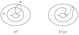
Figure 1: Left: a torus with the cycles $u$, $v$. Right: the action on $v$ of a Dehn twist along the $u$-cycle, represented by the matrix $U$ in (2.7).

This gives the following matrix representation of the two Dehn twists:

$$U=\begin{pmatrix}1&0\\ -1&1\end{pmatrix}\,,\qquad V=\begin{pmatrix}1&1\\ 0&1\end{pmatrix}\,,$$ (2.7)

which indeed satisfy (2.6). We now study a useful classification of elements in $M(T^{2})$. This comes from the characterization of elements in $SL(2,\mathbb{Z})$ inherited by the classification of orientation-preserving isometries of the hyperbolic space, from the identification $PSL(2,\mathbb{R})\approx\text{Isom}^{+}(\mathbb{H}^{2})\approx\text{Isom}^{+}(\text{Teich}(T^{2}))$ given by Möbius transformation. For a given isometry $\phi$ represented by a matrix $M$, the following mutually exclusive possibilities are given:

1. Elliptic type: $\phi$ has one fixed point in $\mathbb{H}^{2}$, or equivalently $|tr(M)|<2$.

2. Parabolic type: $\phi$ has no fixed points in $\mathbb{H}^{2}$ and exactly one fixed point on $\partial\mathbb{H}^{2}$, or equivalently $|tr(M)|=2$.

3. Hyperbolic type: $\phi$ has no fixed points in $\mathbb{H}^{2}$ and exactly two fixed points on $\partial\mathbb{H}^{2}$, or equivalently $|tr(M)|>2$.

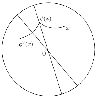
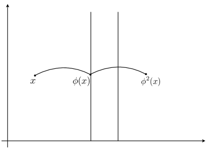
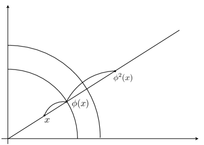
Figure 2: Illustration of the classification of isometries of a two dimensional hyperbolic space. The two lines are the axis of the segment $[\phi(x),\phi^{2}(x)]$, and the bisecting line of the angle between the two segments $[x,\phi(x)]$ and $[\phi(x),\phi^{2}(x)]$. (a) The case of an elliptic map $\phi$ in the disk model $\mathbb{D}^{2}$, with fixed point $0\in\mathbb{D}^{2}$: the two lines are incident. (b) A parabolic map shown in the half-space: the lines are asymptotically parallel. (c) An hyperbolic map: the lines are ultra-parallel. The figures are adapted from [59].

A geometric picture of this classification for $SL(2,\mathbb{R})$ is shown in Figure 2. Note that elliptic elements are necessarily of finite order. We also remark that this trichotomy does not exhaust all conjugacy classes in $SL(2,\mathbb{Z})$. Indeed, there are 6 conjugacy classes of elliptic type, given by the matrices

$$(UV)^{2}=\begin{pmatrix}0&1\\ -1&-1\end{pmatrix}\,,\qquad UVU=\begin{pmatrix}0&1\\ -1&0\end{pmatrix}\,,\qquad UV=\begin{pmatrix}1&1\\ -1&0\end{pmatrix}\,,\qquad$$ (2.8)

respectively of order 3, 4, 6, together with their inverses. Note that from the relations (2.6), the inverses are given by

$$(UV)^{-2} =(UV)^{4}=\begin{pmatrix}-1&-1\\ 1&0\end{pmatrix}\,,\qquad(UVU)^{-1}=(UV)^{4}U=\begin{pmatrix}0&-1\\ 1&0\end{pmatrix}\,,$$

$$(UV)^{-1} =(UV)^{5}=\begin{pmatrix}0&-1\\ 1&1\end{pmatrix}\,.$$ (2.9)

The only other finite order element is $(UV)^{3}=-\mathbb{1}$. For parabolic elements, which are of infinite order, there are infinite conjugacy classes. Note that both the $U$ and $V$ Dehn twists are in the same conjugacy class; a general representative is

$$\pm V^{N}=\pm\begin{pmatrix}1&N\\ 0&1\end{pmatrix}\,.$$ (2.10)

For hyperbolic elements there is a conjugacy class for each value of the trace, plus additional sporadic classes, whose number can be computed by studying equivalence classes of binary quadratic forms, as explained for example in [60]. Two examples are given by

$$V^{1-N}UV=\begin{pmatrix}N&1\\ -1&0\end{pmatrix}\,,\qquad U^{N+1}VU=\begin{pmatrix}0&1\\ -1&-N\end{pmatrix}\,,\quad N\geq 3\,.$$ (2.11)

We also provide a Dehn twist decomposition for the sporadic elements listed in [60] (some of the following matrices are conjugated to their representative matrices):

$$M_{8} =U^{-3}V^{2}=\begin{pmatrix}1&2\\ 3&7\end{pmatrix}\,,\quad M_{10}=U^{-4}V^{2}=\begin{pmatrix}1&2\\ 4&9\end{pmatrix}\,,\quad M_{12}=U^{-5}V^{2}=\begin{pmatrix}1&2\\ 5&11\end{pmatrix}\,,$$

$$M_{13} =U^{2}V^{2}U^{3}V^{3}=\begin{pmatrix}-5&-13\\ 7&18\end{pmatrix}\,,\quad M_{14}=U^{-6}V^{2}=\begin{pmatrix}1&2\\ 6&13\end{pmatrix}\quad+\text{ inverses}\,.$$ (2.12)

The subscript indicates the trace. We note that the decomposition $M_{2N+2}=U^{-N}V^{2}$ seems not to be conjugate to the element (2.11) with the same trace, $V^{-2N-1}UV$, nor to its inverse for $N>1$ so we conjecture that this gives a list of sporadic conjugacy classes for hyperbolic elements of even trace $2N+2$, $N\geq 2$.

The classification obtained from the trace of $SL(2,\mathbb{Z})$ elements is reflected in a trichotomy of the corresponding torus diffeomorphisms. These are periodic, reducible and Anosov maps. We refer to appendix A for a brief review of mapping class groups. A standard result in the theory of 3-manifolds is that the class of torus diffeomorphism $\phi$ determines the geometry of the corresponding mapping torus $\mathcal{N}_{\phi}$, which can be either Euclidean, Nil or Sol. We will see an example of this in the next section.

3 Manifolds and T-folds

We can apply the discussion of the previous section to string theory compactified on a two torus $T^{2}_{\tau}$. An additional fibration on a circle generates a class of 3-manifolds which provides the simplest examples of Nil- and Sol-manifolds. If we also include monodromies in $SL(2,\mathbb{Z})_{\rho}$, classified by an auxiliary $T^{2}_{\rho}$ fibration over the circle, the resulting 3-spaces will be in general non-geometric and are usually referred to as T-folds [62] (see for example [56, 63, 64, 65] for a discussion of such spaces in various contexts). Usually, one arrives to such spaces by performing a chain of T-duality transformations [66, 67]. The simplest example is to start with a three torus $ds^{2}=dx^{2}+dy^{2}+d\theta^{2}$ and a B-field $B=N\theta dx\wedge dy$. Busher rules on $x$ give a metric $ds^{2}=(dx-N\theta dy)^{2}+dy^{2}+d\theta^{2}$ and $B=0$. To make sense of the metric globally one identifies $(x,y,\theta)\sim(x+1,y,\theta)\sim(x,y+1,\theta)\sim(x+Ny,y,\theta+1)$. Note that later in this section and in section 5 we will find more convenient to use conventions for which the period of $\theta$ is $2\pi$. The resulting 3-manifold is a Nil geometry and it is identified with a mapping torus $\mathcal{N}_{\phi}$ for an element $\phi\in SL(2,\mathbb{Z})_{\tau}$ that acts by $\tau\rightarrow\tau+N$. A further application of Busher rules on $y$ gives a metric

$$ds^{2}=f(\theta)(dx^{2}+dy^{2})+d\theta^{2}\,,$$ (3.1)

and a B-field $B=N\theta f(\theta)dx\wedge dy$, with $f(\theta)=(1+N^{2}\theta^{2})^{-1}$. The monodromy is now an element of $SL(2,\mathbb{Z})_{\rho}$ and acts by $\rho^{-1}\rightarrow\rho^{-1}+N$. This has a non-trivial action on the volume, and the corresponding 3-space is a T-fold. The three torus with B-field obviously is not a string vacuum, so this simple example should be considered as an illustrative toy model. An important caveat is the fact that the Nilmanifold is not a principal torus fibration, and the lack of a global $U(1)$ isometry makes the application of Busher rules a priori not obvious. For a detailed discussion on such “obstructed” T-duality see for example [62, 68, 21, 65], and [69] for a discussion on how to possibly overcome this problem.

Our logic will be different and we do not rely on T-duality. In this section, we will classify all possible geometric and non-geometric 3-spaces from the corresponding classification of mapping class groups of the $T^{2}_{\tau}$ and $T^{2}_{\rho}$ fibrations. In the following sections, we will construct explicit solutions for such T-folds and we will use the results of this section to classify all possible local geometries around defects arising from fibration of the T-duality group on $\mathbb{P}^{1}$. The mapping tori we are considering will arise at a boundary of a fibration on a small disk encircling such T-fects. In particular, a subset of mapping class group elements arises from degenerations of elliptic fibrations dual to geometric F-theory compactifications.

We will first briefly review geometric torus bundles with twists in $SL(2,\mathbb{Z})_{\tau}$ and we will then discuss spaces with non-geometric twists.

Figure 3: The mapping torus of a $T^{2}$ compactification. The monodromy of the fibration, that determines the geometry of the total space, is a product of Dehn twists. The simplest example is a twist along one cycle of the homology basis: the total space is a Nilmanifold.

3.1 Geometric monodromies

We now consider a torus fiber with $\rho=i$ fixed and with a complex structure $\tau(\theta)$ varying on $\mathcal{B}=S^{1}$, as shown in Figure 3. This example is elementary and has been discussed in some details in [56] but it serves well to illustrate the role of monodromy. In order to construct the torus fibration, we need to determine the function $\tau(\theta)$, given a monodromy $M\in SL(2,\mathbb{Z})_{\tau}$. The metric of the total space is then:

$$ds_{3}^{2}=d\theta^{2}+G_{ab}(\tau)dx^{a}dx^{b}\,,\quad a=1,2\,,$$ (3.2)

where the torus metric is, from (2.1),

$$G(\tau)=\frac{1}{\tau_{2}}\begin{pmatrix}|\tau|^{2}&\tau_{1}\\ \tau_{1}&1\end{pmatrix}\,,$$ (3.3)

we set $\tau=\tau_{1}+i\tau_{2}$ and we fix the radius of the base circle to $R=1$. Through this section we will set $dx^{1}=dx$, $dx^{2}=dy$. The action of a given element $M$ on $\tau$ is by Möbius transformation (2.2). We fix $\tau_{0}=\tau(0)$ and we demand that $\tau$ has the monodromy $\tau(2\pi)=M[\tau_{0}]$. To find such a function we consider the element $\mathbf{m}=\log(M)$ of the Lie algebra $sl(2,\mathbb{R})$. Then, we construct the path $M(\theta)$ in $SL(2,\mathbb{R})$ given by the exponential map $M(\theta)=\text{exp}(\mathbf{m}\,\theta/2\pi)$. By construction, $M(2\pi)=M$. We define then

$$\tau(\theta)=M(\theta)[\tau_{0}]\,,$$ (3.4)

which obviously has the desired monodromy properties: $\tau(0)=\tau_{0}$, $\tau(2\pi)=M[\tau_{0}]$. We will discuss each of the three classes of $SL(2,\mathbb{Z})_{\tau}$ monodromies, and the corresponding torus diffeomorphisms, separately.

Parabolic (reducible)

We first consider a monodromy of parabolic type, namely an element $M_{\tau}\in SL(2,\mathbb{Z})_{\tau}$ with $|tr(M_{\tau})|=2$. The simplest example is a shift $\tau\rightarrow\tau+N$:

$$M_{\tau}=V^{N}=\begin{pmatrix}1&N\\ 0&1\end{pmatrix}\,,\qquad\mathbf{m}_{\tau}=\begin{pmatrix}0&N\\ 0&0\end{pmatrix}\,.$$ (3.5)

This monodromy implements a $N$-th power of a Dehn twist along the $v$ cycle of the torus once encircling the base and the complex structure is given by $\tau(\theta)=\tau_{0}+N\theta/2\pi$, where $\tau_{0}$ is an arbitrary complex parameter. The corresponding total space is a Nilmanifold. This can be seen from the metric (3.2) which (fixing $\tau_{0}=i$) becomes

$$ds^{2}_{3}=d\theta^{2}+dx^{2}+\left(dy+\frac{N}{2\pi}\theta dx\right)^{2}\,,$$ (3.6)

with the coordinate identification discussed above, that implements the desired monodromy. The metric (3.6) can be written explicitly as a left-invariant metric on a nilpotent Lie group $\mathcal{G}$ as follows. We introduce the Maurer-Cartan forms $\eta^{\theta}=d\theta$ and $\eta^{a}=M(\theta)^{a}_{\phantom{a}b}dx^{b}$, which satisfy:

$$d\eta^{\theta}=0\,,\quad d\eta^{a}=(\mathbf{m}_{\tau})_{\phantom{a}b}^{a}\,\eta^{\theta}\wedge\eta^{b}\,.$$ (3.7)

The generators $(t_{\theta},t_{1},t_{2})$ of the corresponding Lie algebra $\mathfrak{g}$ then satisfy

$$[t_{\theta},t_{a}]=-(\mathbf{m}_{\tau})_{a}^{\phantom{a}b}\,t_{b}\,,\quad[t_{a},t_{b}]=0\,.$$ (3.8)

We see from (3.5) and (3.7) that $\mathfrak{g}$ is the Heisenberg algebra and the torus fibration can also be seen as a principal circle bundle over a torus. The global identification that makes the space compact is a quotient of the Lie group $\mathcal{G}$ by a discrete subgroup. In the notation of [70] this space is referred to as $(0,0,N\times\theta 1)$. The existence of a compactification of the Lie group can be inferred from the condition that the Lie algebra element $\mathbf{m}_{\tau}$ is traceless. The previous example is the simplest example of a Nil geometry and, as we discussed above, it can be obtained by T-duality from a three torus with non-vanishing B-field. We can also consider a monodromy which implements a Dehn twist around the $u$ cycle of the fiber $T^{2}$:

$$M_{\tau}=U^{N}=\begin{pmatrix}1&&0\\ -N&&1\end{pmatrix}\,,\qquad\mathbf{m}_{\tau}=\begin{pmatrix}0&0\\ -N&0\end{pmatrix}\,,$$ (3.9)

which corresponds to the following action on $\tau$:

$$\tau\rightarrow\frac{\tau}{1-N\tau}\,.$$ (3.10)

Note that this corresponds to a shift of $\tau^{-1}$ instead of a shift of $\tau$: $\tau^{-1}\rightarrow\tau^{-1}-N$. More generally, for each $N$ the conjugacy class of a parabolic monodromy is labeled by two coprime integers $(p,q)$:

$$M_{\tau}=L^{-1}V^{N}L=\begin{pmatrix}1+Npq&Np^{2}\\ -Nq^{2}&1-Npq\end{pmatrix}\,,\qquad\mathbf{m}_{\tau}=\begin{pmatrix}Npq&Np^{2}\\ -Nq^{2}&-Npq\end{pmatrix}\,,$$ (3.11)

with $L\in SL(2,\mathbb{Z})$. The corresponding solution for $\tau(\theta)$ is given by:

$$\tau(\theta)=\exp(\mathbf{m}_{\tau}\theta/2\pi)[\tau_{0}]=\frac{(2\pi+Npq\theta)\tau_{0}+Np^{2}\theta}{-Nq^{2}\theta\,\tau_{0}+(2\pi-Npq\theta)}\,.$$ (3.12)

The corresponding metric on the total space is:

$$ds^{2}_{3}=d\theta^{2}+d\tilde{x}^{2}+\left(d\tilde{y}+\frac{N}{2\pi}(p^{2}+q^{2})\theta d\tilde{x}\right)^{2}\,,$$ (3.13)

where

$$\tilde{x}+i\tilde{y}=e^{i\varphi}(x+iy)\,,\quad\varphi=\text{arctan}\left(\frac{q}{p}\right)\,.$$ (3.14)

This is of course the expected result, and the identification of the coordinates now corresponds to gluing the $T^{2}$ after performing a $N$-th power of a Dehn twist along a cycle represented by $p[v]+q[u]$. It is easy to see from (3.8) and (3.11) that the lower central series, namely the sequence of ideals $\mathfrak{g}^{0}=\mathfrak{g},\,\mathfrak{g}^{1}=[\mathfrak{g},\mathfrak{g}^{0}],\,\mathfrak{g}^{2}=[\mathfrak{g},\mathfrak{g}^{1}],\dots$, terminates and the algebra is nilpotent. One might think that different monodromies in the same conjugacy class are uninteresting, however we will see by repeating the previous analysis for twists in $SL(2,\mathbb{Z})_{\rho}$, that parabolic elements in the same class give rise to very different local metrics.

Elliptic (periodic)

We now consider an elliptic conjugacy class represented by the order 4 monodromy:

$$M_{\tau}=UVU=\begin{pmatrix}0&1\\ -1&0\end{pmatrix}\,,\,\qquad\mathbf{m}_{\tau}=\begin{pmatrix}0&\frac{\pi}{2}\\ -\frac{\pi}{2}&0\end{pmatrix}\,.$$ (3.15)

From (3.4) we then find the following solution for $\tau(\theta)$ (see also [56]):

$$\tau(\theta)=\frac{\cos\left(\theta/4\right)\tau_{0}+\sin\left(\theta/4\right)}{-\sin\left(\theta/4\right)\tau_{0}+\cos\left(\theta/4\right)}\,.$$ (3.16)

The corresponding total space is a compactification of the Lie group ISO(2), namely the symmetries of the Euclidean 2-plane. This can be seen from the local coordinates representation of the left-invariant forms:

$$\eta^{\theta} =d\theta\,,$$

$$\eta^{2} =\cos\left(\theta/4\right)dx+\sin\left(\theta/4\right)dy\,,$$

$$\eta^{3} =-\sin\left(\theta/4\right)dx+\cos\left(\theta/4\right)dy\,,$$ (3.17)

which satisfy $d\eta^{\theta}=0,\,d\eta^{1}=\frac{\pi}{2}\eta^{\theta}\wedge\eta^{2},\,d\eta^{2}=-\frac{\pi}{2}\eta^{\theta}\wedge\eta^{1}$. The left-invariant metric is then [56] $ds_{3}^{2}=(\eta^{\theta})^{2}+G_{ab}(\tau_{0})\eta^{a}\eta^{b}$. Analogous results apply to the remaining finite order conjugacy classes. For example, for the conjugacy classes of order 6 and 3, represented by $(UV)^{k}$, $k=1,2$, we have

$$\mathbf{m}_{\tau}^{UV}=\frac{\pi}{3\sqrt{3}}\begin{pmatrix}1&2\\ -2&-1\end{pmatrix}\,,\quad\mathbf{m}_{\tau}^{UVUV}=2\,\mathbf{m}_{\tau}^{UV}\,,$$ (3.18)

and the complex structure is:

$$\tau(\theta)=\frac{A^{+}\tau_{0}+\frac{2}{\sqrt{3}}\sin\left(k\,\theta/6\right)}{-\frac{2}{\sqrt{3}}\sin\left(k\,\theta/6\right)\tau_{0}+A^{-}}\,,\quad A^{\pm}=\cos\left(k\,\theta/6\right)\pm\frac{1}{\sqrt{3}}\sin\left(k\,\theta/6\right)\,.$$ (3.19)

All 3-manifolds obtained in this way are compactifications of Lie groups of a unimodular solvable (but not nilpotent) algebra. Note that if the modulus $\tau_{0}$ is chosen to be the fixed point of the monodromy element, namely

$$UVU:\tau_{0}=i\,,\quad UV:\tau_{0}=e^{i\pi/3}\,,\quad UVUV:\tau_{0}=e^{2i\pi/3}\,,$$ (3.20)

the complex structure does not depend on the circle coordinate and we have $\tau(\theta)=\tau_{0}$. These fixed points are the minima of the potential for the moduli obtained by a reduction with duality twsits and at those points one has a CFT description in terms of symmetric orbifolds. More details can be found in [55, 63, 46, 58].

Hyperbolic (Anosov)

Lastly, we consider hyperbolic monodromies, corresponding to Anosov diffeomorphisms of the fiber torus. Let us first give a simple example with monodromy in $SL(2,\mathbb{R})$:

$$M_{\tau}=\begin{pmatrix}e^{\omega}&0\\ 0&e^{-\omega}\end{pmatrix}\,,\,\qquad\mathbf{m}_{\tau}=\begin{pmatrix}\omega&0\\ 0&-\omega\end{pmatrix}\,.$$ (3.21)

The corresponding modulus is given by $\tau(\theta)=e^{\omega\theta/\pi}\tau_{0}$ and the metric is that of a Sol-manifold. For example, the metric on the total space assuming $\tau_{0}$ is an imaginary parameter is:

$$ds_{3}^{2}=e^{\omega\theta/\pi}dx^{2}+e^{-\omega\theta/\pi}dy^{2}+d\theta^{2}\,.$$ (3.22)

From the relations (3.8) we see that the corresponding algebra is solvable. However, the lower central series generated by $[t_{\theta},\mathfrak{g}]$ for the $sl(2,\mathbb{R})$ element (3.21) do not terminate and thus the algebra is not nilpotent. The compact torus bundle is obtained by a quotient of the Lie group Sol by a discrete subgroup (see for example [61] for more details). Note that the background (3.22) was discussed in [71] and since then Sol-manifolds have played an important role in the search for de Sitter vacua in string theory. Some of the hyperbolic $SL(2,\mathbb{Z})$ conjugacy classes, labeled by an integer $N$ are given by:

$$M_{\tau}=V^{1-N}UV=\begin{pmatrix}N&1\\ -1&0\end{pmatrix}\,,\quad N\geq 3\,.$$ (3.23)

Note that the matrix

$$M=\begin{pmatrix}2&1\\ 1&1\end{pmatrix}\,,$$ (3.24)

representing Arnold’s cat map on the torus, is conjugate to the matrix above for $N=3$. The monodromy matrix can be diagonalized with two eigenvalues ($\lambda$, $1/\lambda$), with

$$\lambda=\frac{1}{2}\left(N+\sqrt{N^{2}-4}\right)\,,\quad N\geq 3\,.$$ (3.25)

Powers of the Anosov diffeomorphism stretch and contract exponentially the two eigenspaces. For this reason, the repackaging of the torus image under powers of an hyperbolic map into the fundamental domain results in a complicate behavior that share many similarities with chaotic systems. We refer to appendix A for a discussion on the dynamics of hyperbolic maps. In terms of $\lambda$ the algebra element is given by

$$\mathbf{m}_{\tau}=\frac{\log\lambda}{\lambda^{2}-1}\begin{pmatrix}\lambda^{2}+1&2\lambda\\ -2\lambda&-(\lambda^{2}+1)\end{pmatrix}\,,$$ (3.26)

and the corresponding modulus is then given by:

$$\tau(\theta)=\frac{\tau_{0}+\lambda-\lambda^{1+\theta/\pi}(1+\lambda\tau_{0})}{-\lambda(\tau_{0}+\lambda)+\lambda^{\theta/\pi}(1+\lambda\tau_{0})}\,.$$ (3.27)

This expression again determines a metric on the total space of the torus bundle. Analogous solutions can be found for the remaining conjugacy classes. Given the peculiar nature of Anosov diffeomorphisms, it would be interesting to revisit phenomenological applications of string models based on hyperbolic torus bundles.

3.2 Non-geometric monodromies

We now discuss the case of a torus bundle in which we fix the complex structure $\tau=i$ of the fiber but we allow $\rho(\theta)$ to vary along the base $\mathcal{B}=S^{1}$. A classification of such spaces can be obtained formally by applying the results of the previous section to an auxiliary $T^{2}_{\rho}$ fibration on the circle, that geometrizes the $SL(2,\mathbb{Z})_{\rho}$ factor of the T-duality group. A local expression for the three dimensional metric and the B-field can be then obtained from:

$$ds_{3}^{2}=d\theta^{2}+\rho_{2}(\theta)(dx^{2}+dy^{2})\,,\quad B=\rho_{1}(\theta)dx\wedge dy\,,$$ (3.28)

where $\rho=\rho_{1}+i\rho_{2}$. With the exception of gauge transformations for the B-field, the monodromy mixes the volume and the B-field, and there is an obstruction to glue the ends of a mapping cylinder with $\rho$ monodromy: the resulting total space will not be a manifold. There exists particular limits in moduli space at which we have a string description of such spaces from asymmetric orbifold CFTs, but otherwise there is no clear string description of such T-folds. Our discussion for now will be formal, but as we will discuss in the next sections, the non-geometric monodromies that we describe do arise in fibrations over $\mathbb{P}^{1}$, and in some cases one could obtain evidence for the existence of the corresponding string vacuum from string dualities.

Parabolic

Let us consider the parabolic monodromy

$$M_{\rho}=V^{N}=\begin{pmatrix}1&N\\ 0&1\end{pmatrix}\,.$$ (3.29)

This corresponds to a shift of $\rho$, giving $\rho(\theta)=\rho_{0}+N\theta/2\pi$ and can be understood geometrically as a power of a Dehn twist along the $v$ cycle of the auxiliary $T^{2}_{\rho}$. The corresponding total space is just a three torus $T^{3}=T^{2}_{\tau}\times S^{1}$ with $N$ units of $H$-flux, and can be obtained by T-duality from the Nilmanifold (3.6) along the global $U(1)$ isometry as we discussed at the beginning of this section. If we consider the conjugate monodromy

$$M_{\rho}=U^{N}=\begin{pmatrix}1&0\\ -N&1\end{pmatrix}\,,$$ (3.30)

we obtain the following solution for $\rho$:

$$\rho(\theta)=\frac{2\pi\rho_{0}}{-N\theta\rho_{0}+2\pi}\,.$$ (3.31)

The gluing condition now mixes the volume of the fiber torus with the B-field, as follows from the action on the volume:

$$\sqrt{G}\rightarrow\frac{\sqrt{G}}{N^{2}G+(NB-1)^{2}}\,.$$ (3.32)

We could consider a fibration of the torus on a interval, but we encounter an obstruction to glue the endpoints to obtain a torus bundle. Note that for $\rho_{0}=i$, from (3.31) we obtain the following metric:

$$ds_{3}^{2}=d\theta^{2}+\frac{4\pi}{4\pi+N^{2}\theta^{2}}\left(dx^{2}+dy^{2}\right)\,,\quad B=-\frac{2\pi N\theta}{4\pi^{2}+N^{2}\theta^{2}}dx\wedge dy\,,$$ (3.33)

which coincides with the T-fold metric we obtain from an obstructed T-duality on the Nilmanifold. We can also consider the general $(p,q)$ parabolic conjugacy class as in (3.12), thus obtaining a class of T-fold metrics that interpolate between the 3-torus and the T-fold.

Elliptic

We can now repeat the analysis of finite order elements done for the geometric $\tau$ monodromies. The corresponding solutions for $\rho(\theta)$, for monodromies of order 3, 4 and 6, are obtained by (3.16) and (3.19) by a fiberwise mirror symmetry $\tau\rightarrow\rho$. The corresponding non-geometric T-folds have been discussed in the context of generalized Scherk-Schwarz reduction within double field theory in [24, 72]. The corresponding potential $V(\rho_{0})$ admits a minimum at the fixed point of the monodromy matrix. At such minimum, there exists a description in terms of an asymmetric orbifold CFT [73, 46]. We note that in the CFT description (as well as in double field theory) we see the presence of both $H$-flux and $Q$-flux. These fluxes should be identified by the corresponding monodromy, the perturbative shift $V_{\rho}\sim H$ and the non-geometric twist $U_{\rho}\sim Q$. The simultaneous presence of both fluxes fits well with the monodromy decomposition of the elliptic monodromy of order 4, $M_{\rho}^{ell}=U_{\rho}V_{\rho}U_{\rho}$. As we will discuss in the next section, such decompositions are defined up to some redundancy, which basically follows from a braid relation of the Dehn twist decomposition. In this case we have for example, from (2.6), $U_{\rho}V_{\rho}U_{\rho}=V_{\rho}U_{\rho}V_{\rho}$, so it is not simple to match the monodromy decomposition with the corresponding flux parameters. We will come back to this point when we will study fibrations on a $\mathbb{P}^{1}$ base and we will identify the sources for the fluxes.

Hyperbolic

The last case is that of a hyperbolic monodromy in $\rho$. A simple example is again obtained by taking the $SL(2,\mathbb{R})$ monodromy (3.21), which for a choice of parameters gives a metric $ds_{3}^{2}=d\theta^{2}+e^{2\theta\omega}(dx^{2}+dy^{2})$. Let us discuss the action on the volume for an $SL(2,\mathbb{Z})$ representative element

$$M_{\rho}=\begin{pmatrix}N&1\\ -1&0\end{pmatrix}\,,\quad N\geq 3\,.$$ (3.34)

The action on $\rho$ is given by

$$\rho\rightarrow-\frac{1}{\rho}-N\,.$$ (3.35)

We note that the action on the volume given by (3.35) is the same as for the elliptic case:

$$\sqrt{G}\rightarrow\frac{\sqrt{G}}{B^{2}+G}\,.$$ (3.36)

However, iterations of the map are not periodic and act in a complicated way. For example, successive iterations act as:

$$\rho\rightarrow-N-\cfrac{1}{-N-\cfrac{1}{\ddots\,-N-\cfrac{1}{\rho}}}\,,$$ (3.37)

and for $N\geq 3$ the continued fraction does not terminate since the fixed points of the transformation are quadratic irrational numbers. The exact expression can be found by setting $\theta=2\pi\,n$ in (3.27) with $\tau\rightarrow\rho$. In terms of the largest eigenvalue $\lambda$ (3.25) we find the following action on the volume:

$$\sqrt{G}\rightarrow\frac{\sqrt{G}\,\lambda^{2n}\,\lambda_{1}^{2}}{(\lambda^{2n}-\lambda^{2})^{2}+2B(\lambda^{2n}-\lambda^{2})\lambda\lambda_{n}+(B^{2}+G)\lambda^{2}\lambda_{n}^{2}}\,,\quad\lambda_{k}=\lambda^{2k}-1\,.$$ (3.38)

Again, we refer to appendix A for more details on the dynamics of hyperbolic diffeomorphisms of surfaces.

3.3 General case

Finally, we briefly discuss the situation in which the full T-duality group is fibered over the circle, and both $\tau(\theta)$ and $\rho(\theta)$ vary. If such configurations are allowed, we can get non-geometric backgrounds which are not fiberwise mirror symmetric to any geometric background. We will discuss the consistency of such configurations in the next sections in relation to heterotic/F-theory duality. We point out that a torus fibration with both $\tau$ and $\rho$ elliptic monodromies has been studied recently in [46, 24]. An example is the order 4 solution:

$$\tau(\theta) =\frac{\cos\left(f\theta\right)\tau_{0}+\sin\left(f\theta\right)}{-\sin\left(f\theta\right)\tau_{0}+\cos\left(f\theta\right)}\,,\quad f\in\frac{1}{4}+\mathbb{Z}\,,$$

$$\rho(\theta) =\frac{\cos\left(g\theta\right)\rho_{0}+\sin\left(g\theta\right)}{-\sin\left(g\theta\right)\rho_{0}+\cos\left(g\theta\right)}\,,\quad g\in\frac{1}{4}+\mathbb{Z}\,.$$ (3.39)

Here the parameters $f$ and $g$ should be identified with geometric and non-geometric fluxes. Such configuration, being not T-dual to a geometric space, can be described in double field theory at the price of relaxing the strong constraint for the generalized Killing vectors. The potential for the moduli $(\tau_{0},\rho_{0})$ has a minimum at the fixed points of the monodromy $(\tau_{0},\rho_{0})=(i,i)$. At this minimum, an asymmetric orbifold description was studied in [46]. We note that the presence of both kind of geometric and non-geometric fluxes should be related in the present context to the factorization of the monodromy in terms of Dehn twists. As we will discuss in more details in the following sections, we should really think in terms of mapping class group of a genus 2 surface obtained by gluing the two tori $T^{2}_{\tau}$, $T^{2}_{\rho}$ with a trivial map. If we then embed the representative matrices $M_{\tau}$, $M_{\rho}$ in $4\times 4$ matrices acting on the homology of the genus-2 surface, we can think about the double elliptic monodromy as being decomposed into $M_{\tau,\rho}^{ell}=U_{\tau}V_{\tau}U_{\tau}U_{\rho}V_{\rho}U_{\rho}$. This would corresponds to having two kind of geometric fluxes, as well as $H$ and $Q$-fluxes, in agreement with the analysis of [46]. We will discuss more about genus 2 fibrations in the last section.

We will now turn to the construction of explicit solutions that provide a concrete realization of the spaces described in this section.

4 T-folds across the wall

Before studying in details fibrations over two-dimensional bases, we mention here a way to embed the 3-spaces discussed in the previous section into backgrounds that solve the supergravity equations of motion. This construction was described in a different context by Hull in [74] and further discussed in [75, 76]. Let us consider the mapping torus with a parabolic monodromy $\tau\rightarrow\tau+N$, namely a Nil-manifold, whose metric is given in (3.6). The latter is determined by the complex modulus $\tau(\theta)=N\theta+\tau_{0}$ (for simplicity in this section we take a periodicity $\theta\sim\theta+1$). We can now make an ansatz for a ten-dimensional metric of the form $\mathbb{R}^{5,1}\times\mathbb{R}\times\mathcal{N}_{3}$, where the mapping torus is fibered over a line parametrized by a coordinate $s$. We then assume that $\tau_{0}$ is a function of $s$:

$$ds^{2}=\eta_{\mu\nu}dx^{\mu}dx^{\nu}+h(s)ds^{2}+R^{2}(s)d\theta^{2}+G_{ab}(\tau(\theta,s))dx^{a}dx^{b}\,,$$ (4.1)

and we further assume that $R^{2}(s)=h(s)$ and $\tau(s)=N\theta+ih(s)$ [74]. The Ricci curvature is then given by

$$R=-\frac{N^{2}-(\partial_{s}h)^{2}+2h\partial_{s}^{2}h}{2h^{3}}\,.$$ (4.2)

It is easy to see that a flat solution which also solves the Ricci-flatness condition is given by $h(s)=Ns+C$, with $C$ an arbitrary constant (see Figure 4). To obtain a sensible solution we can then take the following functions:

$$h(s)=C+s\left[N\Theta(s)-M\Theta(-s)\right]\,,\quad\tau=\left[N\Theta(s)-M\Theta(-s)\right](\theta+is)+iC\,,$$ (4.3)

where $\Theta$ is the step function. For $M=0$ the background becomes:

$$ds^{2}=\eta_{\mu\nu}dx^{\mu}dx^{\nu}+h(s)\left[ds^{2}+d\theta^{2}+dx^{2}\right]+\frac{1}{h(s)}\left[N\Theta(s)\theta dx+dy\right]^{2}\,.$$ (4.4)

Note that at $s=0$ the solution breaks down and there is a curvature singularity $R\sim-N\delta(s)$. As we will discuss in more details in the next section, the background (4.4) corresponds to a KK monopole smeared on two of the $\mathbb{R}^{3}$ directions, and so we should accept the singularity at $s=0$. Alternatively, one can obtain the same solution by first smearing a NS5 brane on a transverse $T^{3}$ and then T-dualize. The solutions clearly make no sense at infinity, much like a D8 brane, and should be regarded as local approximations.

For general $N,M$, the $s=0$ degeneration acts much like the domain-wall D8 brane: it separates two regions with mapping tori of different monodromy.

It is easy to construct the analogous solution with parabolic monodromies in $\rho$. The geometric monodromy $\rho\rightarrow\rho+N$ gives indeed the NS5 brane smeared on a $T^{3}$:

$$ds^{2} =\eta_{\mu\nu}dx^{\mu\nu}+h(s)\left[ds^{2}+d\theta^{2}+dx^{2}+dy^{2}\right]\,,$$ (4.5)

$$B =N\theta\Theta(s)dx\wedge dy\,,\quad e^{2\Phi}=h(s)\,,$$ (4.6)

where $h(s)=C+sN\Theta(s)$ and we made a gauge choice for the $B$-field. A T-fold solution can be obtained starting from the solution (3.31). Since the monodromy is now a perturbative shift in $\rho^{-1}$, we take the following ansatz: $\rho_{0}(s)=h(s)^{-1}$. We then find the following solution:

$$ds^{2} =\eta_{\mu\nu}+h(s)\left[ds^{2}+d\theta^{2}\right]+\frac{h(s)}{1+N^{2}h(s)^{2}}\left[dx^{2}+dy^{2}\right]\,,$$ (4.7)

$$B =\frac{N\theta}{h(s)^{2}+N^{2}\theta^{2}}dx\wedge dy\,,\quad e^{2\Phi}=\frac{h(s)}{1+N^{2}h(s)^{2}}\,.$$ (4.8)

This solution coincides with the T-dual along $y$ of the smeared KK monopole (4.4). Again one could glue T-folds with different monodromies on the two sides of the domain wall. For this reason such defects could be called T-walls.

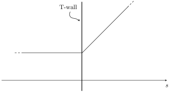
Figure 4: The profile of the harmonic function $h(s)$ for the domain wall considered in the text.

In principle it should be possible to generalize this construction to obtain T-walls with arbitrary T-folds (see [76] for an example with hyperbolic monodromy). However, embedding such local solutions into a global consistent background is not simple, and unless one can understand the degenerations as T-dual of known ones, it is not clear how to discern good and bad singularities. In the next section we will study codimension-2 defects, where a systematic construction of local supergravity solutions is possible for arbitrary T-duality monodromies. Moreover, in some cases the non-geometric fibrations can be understood from string dualities, and this makes possible to eventually put the existence of such backgrounds on more firm ground.

5 Torus fibrations and T-fects

In this section we generalize the previous discussion to the case of a fibration of the T-duality group $O(2,2,\mathbb{Z})$ over a two dimensional base $\mathcal{B}$. This configuration is well known from stringy cosmic strings [14] and was discussed in the context of non-geometric backgrounds in [15]. A complementary point of view, recently described in [11, 12, 13], is to describe the fibrations of the complex structure $\tau$ and the complexified Kähler form $\rho$ in heterotic string theory as elliptic fibrations, and map the corresponding line bundles to an F-theory compactification via heterotic/F-theory duality. A surprising result of this analysis is that even spaces with non-geometric $\rho$ monodromies are mapped to geometric compactifications of F-theory. In such configurations $\tau$ and $\rho$ are meromorphic functions on the base. There is a set of points, that we denote $\Delta=(x_{0},\dots,x_{n})$, at which the fibration degenerates and a defect sits (see Figure 5). These points are branch points for $\tau$ and $\rho$ and there is a nontrivial monodromy around them. Possible degenerations of the elliptic fibrations are described by the Kodaira list as it is familiar in F-theory. Since such defects have T-duality monodromy around them, we will call them generically T-fects.

Here we take a slightly different point of view, with the goal of understanding the relation between the T-folds described in the previous sections and the defects that arise in the case of fibrations over $\mathbb{P}^{1}$. We will consider all possible monodromies in the mapping class group of the compactification torus $T_{\tau}^{2}$ and the auxiliary torus $T^{2}_{\rho}$ and classify the corresponding local solutions. In principle, this classification is more general then the Kodaira classification, since not all of the $SL(2,\mathbb{Z})$ conjugacy classes arise from degenerations of elliptic curves. An illustration of this in F-theory is the case of non-collapsible singularities studied in [60, 77]. We will clarify the relation between these two approaches in a way that can be easily generalized to higher genus fibrations. The latter situation, for genus $g=2$, is of interest in the case of heterotic compactification on a $T^{2}$ with a Wilson line [12] and we outline an interesting geometric perspective on the algebraic classification of genus 2 degenerations [78], as well as a generalization to include non-collapsible defects in this case.

Another outcome of our analysis is the list of all possible geometries arising in a neighborhood of a given $\tau$ and $\rho$ degeneration. In the case of a geometric fibration, some of such geometries can be interpreted as a semi-flat approximation [39, 40] of a class of known ten-dimensional brane solutions, such as the NS5 brane and the KK monopole. In the case of non-geometric fibrations, we recover the exotic brane solution recently discussed in [79, 42]. Our list contains new exotic solutions corresponding to T-fects described by different $SL(2,\mathbb{Z})$ conjugacy classes. As in the case of torus fibrations over a circle, when both $\tau$ and $\rho$ degenerations collide, we found solutions which are not T-dual to a geometric one.

A crucial point that need to be emphasized is about the viability of such local solutions. The solutions alone cannot be taken as automatic evidence that the corresponding degeneration exists in string theory. Put in another way [8, 37, 15], one has to supplement the semi-flat solutions with the knowledge of the microscopic description of a given degeneration, at which the semi-flat approximation breaks down. Once this is understood, the semi-flat torus fibration is a powerful tool to understand physical properties of the corresponding T-fects. One possible point of view is that heterotic/F-theory duality can provide the evidence, even if quite indirect, that non-geometric degenerations should be allowed and in the situations in which enough supersymmetry is preserved, the supergravity solutions should provide a qualitatively correct description.

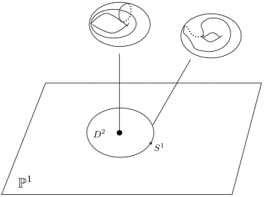
Figure 5: Torus fibration over $\mathbb{P}^{1}$. The mapping torus at the boundary of a small disk $D^{2}$ that encircle a degeneration point determines the local geometry.

Relation to previous works

We note that some of the exotic brane solutions, which correspond to a subset of the solutions for our T-fects, have been described in various places, from different point of views and with a plehtora of different names. We give a short guide to the literature in order to facilitate the comparison with our discussion. As we already mentioned, a parabolic exotic brane usually referred to as $5^{2}_{2}$-brane has been studied in details in [79, 42] and in [43], where it was named Q-brane. Early works include [80, 81, 82]. In [83], parabolic, elliptic and hyperbolic branes were called N, K and A-branes respectively (following an Iwasawa decomposition). Solutions for elliptic and hyperbolic branes for the S-duality $SL(2,\mathbb{Z})$ group have been discussed in [45] for the 7-branes of F-theory, where they are referred to as Q7-branes, and in [84] as solutions of five dimensional supergravity. Elliptic branes were used in [52] as an ingredient to uplift holography and they were referred to as SC5-branes (stringy cosmic five-branes). An elliptic brane was studied in [85] and called $T_{34}$-brane. There have been also more general investigations of codimension-2 solutions, sometimes referred to as “defect branes” (see for example [86, 87, 88]). Here we will simply refer to all the codimension-2 defects with T-duality monodromies as T-fects, emphasizing the relation with the T-folds described in section 3.

5.1 Degenerations and monodromy factorization

Let us briefly describe torus fibrations from the point of view of the mapping class group. The following discussion is in part inspired by the theory of Lefschetz fibrations [89, 90], and we stress that it can be applied to fibrations of surfaces of arbitrary genus. We consider a torus fibration on the punctured sphere $\mathbb{P}^{1}\setminus\Delta$, with $\Delta=(x_{1},\dots,x_{n})$. Let us suppose that at a point $x_{i}$ the fiber degeneration is such that a cycle $p[u]+q[v]$, where $u$ and $v$ is the basis used in section 2, shrinks to zero. The monodromy of the torus fiber around $x_{i}$ is a positive Dehn twist $T_{i}$ along the vanishing cycle and the corresponding action on the homology is given by the Picard-Lefschetz formula (we refer to appendix A for details).

Consider now a disk that encircles some of the degeneration points. If the disk contains the whole $\Delta$, the monodromy around the disk should be homotopic to the identity in order to have a globally defined fibration; otherwise we will have a monodromy $M$, that we can factorize as the product of Dehn twists around each degeneration point: $M=T_{1}\dots T_{n}$, as shown in Figure 6.

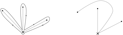
Figure 6: Left: a path that encircle degeneration points (black points) at which a cycle shrinks. A reference smooth point (the cross) is chosen to define the local monodromies. Right: switching the arcs that connect degeneration points and the reference point induce an action by Hurwitz moves on the corresponding monodromy factorization.

This factorization has some gauge redundancy. Locally, we make a choice for defining the monodromy around each points, for example by choosing an arc that connects $x_{i}$ to a given smooth reference point $x_{0}$. The choice is arbitrary, and this results in a equivalence class of monodromy factorizations obtained from the list of vanishing cycles by the action of a braid group $B_{n}$:

$$T_{1}\dots T_{i}T_{i+1}\dots T_{n}\sim T_{1}\dots T_{i}T_{i+1}T_{i}^{-1}T_{i}\dots T_{n}\,,\quad i<n\,.$$ (5.1)

This action is usually called an Hurwitz move and it clearly preserves the global monodromy. We illustrate this in more details in appendix B, where we use it to derive the relation between our Dehn twist factorization for the $SL(2,\mathbb{Z})$ monodromies (2.8), (2.9) and the ABC factorization commonly used in F-theory (in this context the Hurwitz moves arise by moving branch cuts across branes, as in [91]). There is an additional freedom in the choice of the smooth reference fiber over $x_{0}$, which is just a global conjugation on $M$. We arrive at the conclusion that the torus fibration with a fixed number of elementary degenerations is defined by the factorization of the global monodromy up to Hurwitz moves and global conjugation.

In general, the degeneration of a torus fiber can be worse then a simple shrinking cycle. The classification of such degenerations are well known from the Kodaira classification of singular fibers for elliptic fibrations that we briefly review in appendix B. However, the generalization to fibrations of higher genus is much more involved, see [78, 12, 13] for a discussion of the genus 2 case.

Given the geometric group approach we described above, it is natural to ask whether one can give a more geometric description of such classification from the point of view of fiber diffeomorphisms. Note that for the torus fibration a classification of periodic diffeomorphisms, i.e. elliptic $SL(2,\mathbb{Z})$ conjugacy classes, is in correspondence with the Kodaira list with the exception of $I,I^{\ast}$ fibers, which instead corresponds to the parabolic class, but no hyperbolic (Anosov) monodromy arises from degenerating elliptic fibers. It turns out that such a geometric approach exists as a result of an elaborated theorem [38]. For genus $g\geq 2$, there is a bijection between degenerations of a family of Riemann surfaces (up to an appropriately defined topological equivalence relation) and a subset of conjugacy classes of the mapping class group of the fiber, given by pseudo-periodic elements. For the torus, the map is surjective. We refer to appendix A for a definition of pseudo-periodic mapping classes, but this subset basically contains parabolic and elliptic elements. We anticipate that this geometric point of view will be useful to generalize our presentation to the genus 2 case, relevant for non-geometric backgrounds of the heterotic theory with a Wilson line.

Note that for lower genus fibrations, known facts about mapping class groups can be also helpful to determine possible global models. For example, one can show that for torus fibrations it is not possible to factorize the identity with less then 12 Dehn twists. This corresponds to the defining relation (2.6) for the presentation of the mapping class group $M(T^{2})$. We can think of a word in the $U,V$ alphabet that factorizes the identity as defining a global fibration in which the total charge is canceled. Some of the elementary constituents can then be collapsed into one of the Kodaira degenerations if their total monodromy is elliptic or parabolic. However, one can still imagine situations in which a group of non-collapsed branes gives rise to a hyperbolic monodromy.

We now turn to a classification of all possible local geometries that arise in our model, both for the geometric $T^{2}_{\tau}$ and the auxiliary $T^{2}_{\rho}$ fibrations. The complex and Kähler moduli $\tau$ and $\rho$ should really be thought as functions on an appropriate multi-sheeted Riemann surface, where the transition between sheets is determined by a given $SL(2,\mathbb{Z})$ element, that we identify with an element in $M(T^{2})$. We construct the local solutions by taking the mapping torus $\mathcal{N}_{\phi}$ (2.5) for a given $\phi\in M(T^{2})$ in each conjugacy class, and we then solve the Cauchy-Riemann equations to obtain a meromorphic function with the desired monodromy. This determines a semi-flat approximation of the corresponding T-fect. For parabolic and elliptic conjugacy class, we will recover in this way the known local solutions that already appeared in the work of Kodaira [36], see Table 1. These can be obtained by inverting Klein’s $j$ modular function that specify a given global elliptic fibration. Inserted in the appropriate semi-flat ansatz, we obtain the corresponding geometric and non-geometric local solutions. Note however that interesting solutions can arise from different monodromies in the same conjugacy class, so we also need to determine the general form of the meromorphic functions. Solutions for hyperbolic monodromies are substantially more complicated and cannot be found by other simple methods.

Class	Type	Monodromy	Local model
Parabolic	$I_{n}$	$V^{n}=\begin{pmatrix}1&n\\ 0&1\end{pmatrix}$	$\displaystyle\frac{n}{2\pi i}\log z\,,\quad n>0$
Elliptic order 6	$II$	$UV=\begin{pmatrix}1&1\\ -1&0\end{pmatrix}$	$\displaystyle\frac{\eta-\eta^{2}z^{1/3}}{1-z^{1/3}}\,,\quad\eta=e^{2\pi i/3}$
Elliptic order 4	$III$	$UVU=\begin{pmatrix}0&1\\ -1&0\end{pmatrix}$	$\displaystyle\frac{i+i\sqrt{z}}{1-\sqrt{z}}$
Elliptic order 3	$IV$	$UVUV=\begin{pmatrix}0&1\\ -1&-1\end{pmatrix}$	$\displaystyle\frac{\eta-\eta^{2}z^{2/3}}{1-z^{2/3}}$

Table 1: Local solutions around degenerations of Kodaira type $I_{n}$, $II$, $III$, $IV$.

5.2 Geometric $\tau$-fects

We now discuss local solutions in neighborhoods of degenerations for the $\tau$ fibration. We consider the complexified Kähler parameter fixed to $\rho=i$, while $\tau(z)$ will now be a function on a two dimensional base $\mathcal{B}$ with complex coordinate $z=re^{i\theta}$. We assume a semi-flat metric ansatz $\mathbb{R}^{1,5}\times\mathcal{B}\times_{\varphi}T^{2}$, where $T^{2}$ is fibered over $\mathcal{B}$ and we preserves the $U(1)\times U(1)$ isometries of the fiber torus:

$$ds^{2}_{10} =\eta_{\mu\nu}dx^{\mu}dx^{\nu}+e^{2\varphi_{1}}\tau_{2}dzd\bar{z}+G_{ab}(z)dx^{a}dx^{b}\,,$$

$$\qquad e^{2\Phi} =\text{const}\,,\qquad B=0\,\qquad\mu,\nu=0,\dots 5\,,\quad a,b=8,9\,,$$ (5.2)

where

$$G(z)=\frac{1}{\tau_{2}}\begin{pmatrix}|\tau|^{2}&\tau_{1}\\ \tau_{1}&1\end{pmatrix}\,.$$ (5.3)

Here $\varphi=\varphi_{1}+i\varphi_{2}$ and $\tau=\tau_{1}+i\tau_{2}$ are meromorphic functions on $\mathcal{B}$. We will mainly focus on a local description with $\mathcal{B}$ a disk. Such local solutions can then be glued to obtain a global fibration on $\mathbb{P}^{1}$. As we will discuss later for the general case of arbitrary $\rho$, it is easy to show that the second-order equations of motion are implied by holomorphicity of $\tau$ and $\varphi$. One can also show that such condition is enough to preserve half of the supersymmetries [15, 45, 42]. We assume a branch point at the origin where the description will break down and we have to resort to a string description of the degeneration. Given a small disk $D^{2}:0<\lvert z\rvert<R_{0}$ that contains the origin, we consider the smooth torus fibration on the boundary $S^{1}=\partial D^{2}$. These are the fibrations that we classified in section 3, namely mapping tori for a given mapping class group element, that we identify with the monodromy of the multi-valued function $\tau(z)$, up to the kernel $\{\pm\mathbb{1}\}$. Given such monodromy, a local solution for $\tau(z)$ can be found by solving the Cauchy-Riemann equations by separation of variables. Namely, we start with the solutions for mapping tori derived in section 3.1 and we promote the free modulus $\tau_{0}$ of such solutions to a function of $r=\lvert z\rvert$. The equations then reduce to an ordinary differential equation for $\tau_{0}(r)$. We will see that a solution always exists for all the three different classes of the fiber diffeomorphism on $\partial D^{2}$. Thus, given a monodromy

$$M_{\tau}=\begin{pmatrix}a&b\\ c&d\end{pmatrix}\,,\quad ad-bc=1\,,$$ (5.4)

we obtain a function $\tau(z)$ such that the analytic continuation along an arc that encircles the origin is

$$\tau(z)\rightarrow\frac{a\tau(z)+b}{c\tau(z)+d}\,.$$ (5.5)

We still have to solve for the warping factor $\varphi(z)$. By various arguments [15, 45, 42], one can show that in order for the metric on $\mathcal{B}$ to be single-valued the analytic continuation for $\varphi$ should be

$$e^{\varphi(z)}\rightarrow e^{\varphi(z)}(c\,\tau(z)+d)\,.$$ (5.6)

Again, once $\tau(z)$ is known, one can solve the equation for $\varphi$ by separation of variables. We note that in many cases one can easily guess the solution with the given monodromy, but there are few exceptions which are more complicated.

Parabolic $\tau$-fects and KK monopoles

We consider the situation in which the tours fiber degenerates at $z_{0}=0$ by shrinking a cycle $p[v]+q[u]$. If $q=0$ and $p=1$ we have the monodromy (3.5) for $N=1$, $M_{\tau}=V$. The corresponding action on $\tau$ is a shift:

$$\tau\rightarrow\tau+1\,.$$ (5.7)

The corresponding solution is of course well known [14]:

$$\tau(z)=\frac{i}{2\pi}\log\left(\frac{\mu}{z}\right)\,,\qquad e^{\varphi}=1\,,$$ (5.8)

where $\mu$ is an integration constant. The corresponding metric in polar coordinates on $\mathcal{B}$ is thus:

$$ds^{2} =\eta_{\mu\nu}dx^{\mu}dx^{\nu}+\frac{1}{2\pi}\log\left(\frac{\mu}{r}\right)\left[d\theta^{2}+r^{2}dr^{2}+(dx^{8})^{2}\right]$$

$$\quad+\frac{2\pi}{\log\left(\frac{\mu}{r}\right)}\left(dx^{9}+\frac{\theta}{2\pi}dx^{8}\right)^{2}\,.$$ (5.9)

It is easy to check that this is a semi-flat approximation of a KK monopole with compact circle $x^{9}\approx u$. Indeed, this is precisely the analysis done in [92]. To show this, let us start from the Taub-NUT metric:

$$ds^{2}_{KKM}=\eta_{\mu\nu}dx^{\mu}dx^{\nu}+V(\vec{x})\,d\vec{x}^{2}+\frac{1}{V(\vec{x})}\left(dx^{9}+A\right)^{2}\,,\qquad V(\vec{x})=1+\frac{R_{9}}{2|\vec{x}|}\,,$$ (5.10)

where $A=\vec{A}\cdot d\vec{x}$, $\vec{x}=(z,\bar{z},x^{8})$, and $dA=*_{3}dV$. We will set the radius $R_{9}=1$. We now compactify on $x^{8}$. This corresponds to have an infinite array of sources on the covering space, resulting in the potential:

$$V=\frac{1}{2}\sum_{n=-\infty}^{\infty}\left[\frac{1}{\sqrt{(x_{8}-2\pi n)^{2}+r^{2}}}-\frac{1}{|2\pi n\rvert}\right]\,,$$ (5.11)

where we added a regulator. This sum can be performed exactly by Poisson resummation [92], resulting in:

$$V=\frac{1}{2\pi}\left[\log(\mu/r)+\sum_{n\neq 0}e^{inx^{8}}K_{0}\left(\lvert n\rvert r\right)\right]\,,$$ (5.12)

where $K_{0}$ is the modified Bessel function. Away from the origin, the leading order is a very good approximation (up to the exponentially suppressed terms), and the metric with this leading order approximation to $V$ reduces precisely to the semi-flat metric (5.9). The half-cigar of the Taub-NUT space became a pinched torus obtained from the shrinking of the $u$ cycle (see Figure 7).

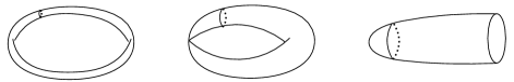
Figure 7: From left to right: the semi-flat degeneration of a KK monopole, the localized solution and the decompactified half-cigar of the Taub-NUT space.

This analysis can be easily extended to the monodromy $V^{N}$, which corresponds to having a stack of $N$ KK monopoles at the degeneration point. We now consider the generic case corresponding to the $(p,q)$ parabolic conjugacy class, with $q\neq 0$:

$$M_{\tau}=\begin{pmatrix}1+pq&p^{2}\\ -q^{2}&1-pq\end{pmatrix}\,.$$ (5.13)

We also list the embedding into the $O(2,2,\mathbb{Z})$ group (see appendix D for a short review):

$$\Omega_{O(2,2)}=\begin{pmatrix}1+pq&p^{2}&0&0\\ -q^{2}&1-pq&0&0\\ 0&0&1-pq&q^{2}\\ 0&0&-p^{2}&1+pq\end{pmatrix}\,.$$ (5.14)

To find the appropriate meromorphic function we consider the following ansatz for $\tau(r,\theta)$:

$$\tau(r,\theta)=\exp(\mathbf{m}_{\tau}\theta/2\pi)[\tau_{0}(r)]\,,$$ (5.15)

where $\mathbf{m}_{\tau}$ is the element of the $sl(2,\mathbb{Z})$ Lie algebra defined in (3.11). By plugging this ansatz into the Cauchy-Riemann equations

$$\frac{\partial\tau(r,\theta)}{\partial r}-\frac{1}{ir}\frac{\partial\tau(r,\theta)}{\partial\theta}=0\,,$$ (5.16)

we see that they reduce to a single ordinary differential equation for $\tau_{0}(r)$:

$$2\pi ir\frac{d\tau_{0}(r)}{dr}=\big{[}p+q\tau_{0}(r)\big{]}^{2}\,.$$ (5.17)

We then find a solution for $\tau(z)$:

$$\tau(z)=\frac{2\pi i}{q^{2}\log\left(\frac{\mu}{z}\right)}-\frac{p}{q}\,.$$ (5.18)

By making an analogous ansatz for $e^{\varphi(z)}$ we obtain:

$$e^{\varphi(z)}=i\kappa\log\left(\frac{\mu}{z}\right)\,,$$ (5.19)

where $\kappa$ is an arbitrary integration constant. Since the monodromy corresponds now to a Dehn twist along the vanishing cycle $p[u]+q[v]$, we obtain a semi-flat approximation of a KK monopole with special circle an oblique direction in the $(x^{8},\,x^{9})$ plane whose slope is determined by the ratio $q/p$, as in (3.14). The semi-flat approximation arises after compactifying the orthogonal direction and taking the leading approximation for V as discussed before.

Elliptic $\tau$-fects

We now consider the case in which the monodromy around the degeneration is of finite order, corresponding to a periodic diffeomorphism of the torus. Different degenerations are classified by the conjugacy classes of elliptic $SL(2,\mathbb{Z})$ elements and are listed in (2.8), (2.9). We consider for illustration the monodromy of order 4: $M_{\tau}=UVU$ ($\tau\rightarrow-1/\tau$), that corresponds to the following $O(2,2,\mathbb{Z})$ element:

$$\Omega_{O(2,2)}=\begin{pmatrix}0&1&0&0\\ -1&0&0&0\\ 0&0&0&1\\ 0&0&-1&0\end{pmatrix}\,.$$ (5.20)

The solution for $\tau(\theta)$ for a fibration on a circle is (3.16). The Cauchy-Riemann equations coming from the ansatz (5.15) and the analogous for $e^{\varphi}$ reduce to:

$$4r\frac{d\tau_{0}}{dr}+i(\tau_{0}^{2}+1)=0\,,\qquad 4r\frac{d\varphi_{0}}{dr}=i\tau_{0}\phi_{0}\,.$$ (5.21)

From this we obtain the following solutions:

$$\tau(z)=\tan\left[C-\frac{i}{4}\log(z)\right]\,,\qquad e^{\varphi(z)}=\kappa\cos\left[C-\frac{i}{4}\log(z)\right]\,,$$ (5.22)

where $C$ and $\kappa$ are integration constants. Note that the solution for $\tau$ can be rewritten as

$$\tau(z)=\frac{i-ie^{2iC}\sqrt{z}}{1-ie^{2iC}\sqrt{z}}=i-2ie^{2iC}\sqrt{\frac{z}{\mu}}+2ie^{4iC}z+\mathcal{O}(z^{3/2})\,,$$ (5.23)

For $C=\pi/2$ the solution for $\tau$ reproduces the local model shown in Table 1. At the degeneration point the complex modulus is given, as expected, by the fixed point of the elliptic monodromy, $\tau_{0}=i$. The metric for the total space can then be easily found from (5.2).

As for the parabolic case, we could also consider solutions associated to the general conjugacy class of the particular elliptic monodromy. This is specified by three parameters $(p,q,w)$:

$$M_{p,q,w}=L^{-1}UVUL=\begin{pmatrix}\displaystyle pq+\frac{w(1+qw)}{p}&\displaystyle p^{2}+w^{2}\\ \displaystyle-q^{2}-\frac{(1+qw)^{2}}{p^{2}}&\displaystyle-\frac{w+q(p^{2}+w^{2})}{p}\end{pmatrix}\,,$$ (5.24)

for $L\in SL(2,\mathbb{Z})$. By constructing the fibration on a $S^{1}$ from (3.4), we find a general solution of the Cauchy-Riemann equations for $\tau(z)$ and $e^{\varphi(z)}$:

$$\tau(z) =w\left[\frac{1}{p+w\tan\left[p^{2}\,C-\frac{i}{4}\log(z)\right]}-\frac{1+wq}{p}\right]^{-1}\,,$$ (5.25)

$$e^{\varphi(z)} =\kappa\,p\,q\cos\left[p^{2}\,C-\frac{i}{4}\log(z)\right]+\kappa\,i(1+p\,w)\sin\left[p^{2}\,C-\frac{i}{4}\log(z)\right]\,.$$ (5.26)

A similar analysis can be done for all the remaining elliptic conjugacy classes. For example, the solutions corresponding to the monodromy $UV$ and $(UV)^{2}$ can be found by starting from the solution (3.19). The results are:

$$UV :\quad\tau(z)=\frac{\eta+\eta^{2}e^{iC}z^{1/3}}{1+e^{iC}z^{1/3}}\,,\qquad e^{\varphi(z)}=\kappa\left(e^{-iC/2}z^{-1/6}+e^{iC/2}z^{1/6}\right)\,,$$ (5.27)

$$UVUV :\quad\tau(z)=\frac{\eta+\eta^{2}e^{iC}z^{2/3}}{1+e^{iC}z^{2/3}}\,,\qquad e^{\varphi(z)}=\kappa\left(e^{-iC/2}z^{-1/3}+e^{iC/2}z^{1/3}\right)\,,$$ (5.28)

from which the metric can be easily reconstructed. For $C=\pi$ these solutions are listed in Table 1.

We note that in a given global model for an elliptic fibration specified by a Weierstrass form

$$y^{2}=x^{3}+f(z)x+g(z)\,,$$ (5.29)

the function $\tau(z)$ is specified implicitly by Klein’s $j$-invariant:

$$j(\tau)=\frac{(12f)^{3}}{4f^{3}+27g^{2}}\,.$$ (5.30)

In general, there will be degeneration points located at the discriminant locus $\Delta:4f^{3}+27g^{2}=0$. The solution for $\tau$ around poles of the $j$-function are the parabolic solutions (namely KK monopoles in our case), while around removable singularities for $j(\tau)$ the solutions are approximated by the elliptic solutions described above. In the next paragraph, we will study hyperbolic solutions that cannot arise in this simple situation.

Hyperbolic $\tau$-fects

The last example is that of a hyperbolic monodromy, corresponding to an Anosov map of the fiber torus. A simple example with monodromy in $SL(2,\mathbb{R})$ is given by the matrix (3.21). In this case we trivially obtain:

$$\tau(z)=z^{-iw/\pi}\,,\qquad e^{\varphi(z)}=z^{iw/2\pi}\,.$$ (5.31)

Note that the imaginary part of $\tau$ is a periodic function of $\log(r)$, so it has a highly oscillatory behavior near the origin. The solutions for conjugacy classes of hyperbolic $SL(2,\mathbb{Z})$ monodromies are more involved but share the same problem. As an example, for the monodromy (3.23), which corresponds to the $O(2,2,\mathbb{Z})$ element

$$\Omega_{O(2,2)}=\begin{pmatrix}N&1&0&0\\ -1&0&0&0\\ 0&0&0&1\\ 0&0&-1&N\end{pmatrix}\,,$$ (5.32)

we obtain the following differential equations:

$$\pi r(\lambda^{2}-1)\frac{d\tau_{0}(r)}{dr}+i\log(\lambda)\left[\lambda+\tau_{0}(r)\right]\left[\lambda\tau_{0}(r)+1\right] =0\,,$$ (5.33)

$$2\pi r(\lambda^{2}-1)\frac{d\phi_{0}(r)}{dr}-i\log(\lambda)\left[1+\lambda^{2}+2\lambda\tau_{0}(r)\right]\phi_{0}(r) =0\,.$$ (5.34)

The solutions can be written explicitly:

$$\tau(z) =\frac{\sigma^{\lambda^{2}}(\lambda^{2}-1)}{\lambda(\sigma e^{i\tilde{z}}-\sigma^{\lambda^{2}})}-\frac{1}{\lambda}\,,$$ (5.35)

$$e^{\phi(z)} =\kappa\sqrt{\lambda}e^{\frac{i}{2}(\mu-\tilde{z}\lambda^{2})}\left[\sigma^{\lambda^{2}}-\sigma e^{i\tilde{z}}\right]\,,$$ (5.36)

where $\sigma,$ $\mu$, $\kappa$ are integration constants and we defined

$$\tilde{z}=\mu(1-\lambda^{2})+\frac{1}{\pi}\log\lambda\log\left[\pi z(\lambda^{2}-1)\right]\,.$$ (5.37)

It is not obvious how to make sense of such solutions near the origin, since there are infinite intervals at which $\tau_{2}<0$. This fits well with the fact that Anosov diffeomorphisms cannot be obtained as monodromies of a degenerating family of curves, and thus cannot be associated with a degeneration point. The F-theory analogous of such hyperbolic branes appeared in [77, 60]. In the F-theory context, there are separated 7-branes, and the associated massive states gives rise to infinite dimensional algebras. We note that the previous solution might approximates a non-collapsed group of branes, that can be identified by the Dehn twist decomposition given in section 2. In this way there is a scale representing the size of the brane distribution which serves as a cutoff around the origin for our solution. This is reminiscent of an enhano̧n mechanism [94]. To cure the problem at infinity, one should put additional defects in order to cancel the total charge, as for all the other co-dimension 2 defects. To show that this is possible in the presence of a hyperbolic monodromy, let us for example consider a model with the following $SL(2,\mathbb{Z})$ elements:

$$M_{H}=U^{4}VU=\begin{pmatrix}0&1\\ -1&-3\end{pmatrix}\,,\quad M_{1}=UV^{2}=\begin{pmatrix}1&2\\ -1&-1\end{pmatrix}\,,\quad M_{2}=U^{2}V=\begin{pmatrix}1&1\\ -2&-1\end{pmatrix}\,,$$

where $M_{1}$ and $M_{2}$, are elliptic monodromies of order 4, both conjugate to the Kodaira degeneration $III=UVU$. We then check that they provide a factorization of the identity:

$$M_{H}M_{1}M_{2}=\mathbb{1}\,.$$ (5.38)

Note that as expected, the total number of elementary branes is 12. One can add an additional factorization $(UV)^{6}=\mathbb{1}$ to obtain a model with 24 branes. It would be interesting to understand better the nature of the hyperbolic solutions in the present context.

5.3 Exotic $\rho$-fects

In the previous section we discussed a classification of local geometries associated to monodromies filling the $SL(2,\mathbb{Z})_{\tau}$ mapping class group of the compactification torus. Global models of such $\tau$ fibrations give rise to geometric six dimensional compactifications. We now consider the case of a $\rho$ fibration, that can be geometrized as a mapping class group of an auxiliary torus. The $\rho$ fibrations, at constant $\tau=i$, are the fiberwise mirror-symmetric of the geometric solutions discussed above. The semi-flat metric ansatz in this case reads:

$$ds^{2}_{10} =\eta_{\mu\nu}dx^{\mu}dx^{\nu}+e^{2\varphi_{1}}\rho_{2}dzd\bar{z}+\rho_{2}(dx_{8}^{2}+dx_{9}^{2})\,,$$ (5.39)

$$B =\rho_{1}dx_{8}\wedge dx_{9}\,,\qquad e^{2\Phi}=\rho_{2}\,.$$

Note that this is a concrete realization of the fibration (3.28). The fact that the base circle now becomes contractible in the two dimensional base $\mathcal{B}$ provides the necessary gradient terms to solve the equations of motion. This is similar to the T-walls discussed in section 4 but we now have codimension-2 defects at points where the $\rho$ fibration degenerates. Again, the second-order equations are implied by the Cauchy-Riemann equations for $\varphi(z)$ and $\rho(z)$, as can be shown from the supersymmetry analysis performed in details in [15, 42, 41]. In appendix C we independently check that the previous ansatz solves the equations of motion. One should keep in mind that at the degeneration points of the auxiliary $T^{2}_{\rho}$ fibration, namely branch points for $\rho(z)$, this description breaks down and we have to resort to a string description. Note that since the dilaton is running, one should also check that it transforms in the correct way under T-duality once encircling the defect. This is indeed the case for the ansatz (5.39).

Parabolic $\rho$-fects: NS5 and $5^{2}_{2}$ branes

The meromorphic solutions derived in the previous section automatically define, by just exchanging $\tau\rightarrow\rho$, a local supersymmetric solution of the supergravity equations, of the form (5.39). The simplest situation is that of a parabolic monodromy of type $V^{N}$. This corresponds to gluing the torus with a gauge transformation for the B-field, so the corresponding solution is geometric. We have

$$\rho(z)=\frac{i}{2\pi}\log\left(\frac{\mu}{z}\right)\,,\qquad e^{\varphi}=1\,,$$ (5.40)

and the background metric is then:

$$ds^{2} =\eta_{\mu\nu}dx^{\mu}dx^{\nu}+\frac{1}{2\pi}\log\left(\frac{\mu}{r}\right)\left[d\theta^{2}+r^{2}dr^{2}+(dx^{8})^{2}+(dx^{9})^{2}\right]\,.$$ (5.41)

$$B =\frac{\theta}{2\pi}dx^{8}\wedge dx^{9}\,,\qquad e^{2\Phi}=\frac{1}{2\pi}\log\left(\frac{\mu}{r}\right)\,.$$ (5.42)

As it is well known, this solution can be identified with the semi-flat approximation of a stack of NS5 branes [37] (see also  [40, 42]). To show this we can follow the same steps as for the case of the KK monopole in the previous section. The solution for a stack of NS5 branes localized on $\mathbb{R}^{2}\times T^{2}$ can be found by starting from the NS5 harmonic function $h$ and compactify two directions, which is equivalent to consider an array of sources on the $(x^{8},x^{9})$ plane. This gives

$$h(r)=\sum_{n,m}\frac{1}{(x^{8}-2\pi n)^{2}+(x^{9}-2\pi m)^{2}+r^{2}}+\text{regulator}\,.$$ (5.43)

At distances large compared to the distance between the sources, the result for the harmonic function is clearly the same as the smeared KK monopole, and we obtain the metric (5.41). However, note that the corrections to the semi-flat approximation involve the breaking of both the $U(1)$ isometries of the torus (see [41] for a field theory computation of such corrections) . It would be interesting to understand if this localization is encoded in the auxiliary $T^{2}_{\rho}$ fibration. Since the degeneration is the same as for the KKM, it seems that information about the breaking of the second $U(1)$ isometry is missing. We will come back shortly on this point. First, we consider the solutions for the general conjugacy class of parabolic $\rho$ monodromies, namely the ones associated to a $(p,q)$ monodromy

$$M_{\rho}=\begin{pmatrix}1+pq&p^{2}\\ -q^{2}&1-pq\end{pmatrix}\,.$$ (5.44)

We also show the corresponding $O(2,2,\mathbb{Z})$ element:

$$\Omega_{O(2,2)}=\begin{pmatrix}1+pq&0&0&p^{2}\\ 0&1+pq&-p^{2}&0\\ 0&q^{2}&1-pq&0\\ -q^{2}&0&0&1-pq\end{pmatrix}\,.$$ (5.45)

Note that for $p=0$ the monodromy is a $\beta$-transformation (see Appendix D), while for $q=0$ this is just a B-transformation. For general $p,q$ both transformations are present at the same time. The NS5 brane corresponds to a $(1,0)$ brane, while the general solution for $q\neq 0$ can be obtained from (5.18), (5.19). The $(0,1)$ solution, with monodromy $U^{N}$ ($1/\rho\rightarrow 1/\rho+1$) is

$$\rho(z)=\frac{2\pi i}{\log\left(\frac{\mu}{z}\right)}\,,\qquad e^{\varphi}=i\sigma\log{\left(\frac{\mu}{z}\right)}\,.$$ (5.46)

We then get the following solution:

$$ds^{2}_{10} =\eta_{\mu\nu}dx^{\mu}dx^{\nu}+2\pi\sigma^{2}h(r)(dr^{2}+r^{2}d\theta^{2})+\frac{2\pi h(r)}{h(r)^{2}+\theta^{2}}\left[(dx^{8})^{2}+(dx^{9})^{2}\right]\,,$$ (5.47)

$$B =-\frac{2\pi\theta}{h(r)^{2}+\theta^{2}}dx^{8}\wedge dx^{9}\,,\qquad e^{2\Phi}=\frac{2\pi h(r)}{h(r)^{2}+\theta^{2}}\,,$$

where

$$h(r)=\log\left(\frac{\mu}{r}\right)\,.$$ (5.48)

We see that the monodromy acts non-trivially on the volume, so this solution is non-geometric. This is the exotic brane solution recently discussed in length in [42] (see also [43]) and usually called Q-brane or $5^{2}_{2}$-brane in the notation of [80]. We have explicitly shown that at the boundary of a small neighborhood of such exotic brane, the torus fibers on the boundary of the disk as in the parabolic T-fold fibrations. Since the latter background con only be obtained from an obstructed T-duality from a Nilmanifold, it is interesting to obtain a solution with the same monodromy from a different perspective.

Note that also the metric (5.47) can be obtained by applying Busher rules to the semi-flat KKM metric (5.8), in the same way the NS5 smeared on one circle is T-dual to the KKM solution (5.10). In the latter case, correction to the Busher rules coming from the breaking of the $U(1)$ smearing isometry can be computed as worldsheet instantons corrections [95, 96]. It is clearly very important to understand the breaking of the $U(1)$ isometry in the case of the second T-duality that relate the KKM to the metric (5.47). This is analogous to understand the corrections to the semi-flat approximation for the auxiliary $\rho$ fibrations.

Elliptic $\rho$-fects

If we now consider elliptic monodromies of finite orders, we can again obtain local solutions from the functions (5.22), (5.26), (5.27) and analogous solutions for other conjugacy classes. For example, the order 4 monodromy $M_{\rho}=UVU$ corresponds to the following background:

$$ds^{2} =\eta_{\mu\nu}dx^{\mu}dx^{\nu}-\frac{1}{2}\sinh\left[\frac{1}{2}\log\left(\frac{r}{\mu}\right)\right](dr^{2}+r^{2}d\theta^{2})$$

$$\quad-\frac{\sinh\left[\frac{1}{2}\log\left(\frac{r}{\mu}\right)\right]}{\cos\left(\frac{\theta}{2}+\sigma\right)+\cosh\left[\frac{1}{2}\log\left(\frac{r}{\mu}\right)\right]}\left[(dx^{8})^{2}+(dx^{9})^{2}\right]\,,$$ (5.49)

$$B_{2} =-\frac{\sin(\theta/2+\sigma)}{\cos(\theta/2+\sigma)+\cosh\left[\frac{1}{2}\log\left(\frac{\mu}{r}\right)\right]}dx^{8}\wedge dx^{9}\,,$$

$$e^{2\Phi} =-\frac{\sinh\left[\frac{1}{2}\log\left(\frac{r}{\mu}\right)\right]}{\cos\left(\frac{\theta}{2}+\sigma\right)+\cosh\left[\frac{1}{2}\log\left(\frac{r}{\mu}\right)\right]}\,.$$ (5.50)

Compared to the solution (5.22) we redefined $C_{1}=\sigma$, $C_{2}=1/4\log(\mu)$. Let us check explicitly that the solution has the desired monodromy. The action of the elliptic transformation is $\rho\rightarrow-1/\rho$. Recalling that $\rho=B+i\sqrt{G}$, this corresponds to:

$$B(2\pi)=-\frac{B(0)}{B(0)^{2}+G(0)}\,,\qquad\sqrt{G}(2\pi)=\frac{\sqrt{G}(0)}{B(0)^{2}+G(0)}\,,$$ (5.51)

where we indicated in brackets the value of the angle $\theta$ at which the fields are evaluated. It is not difficult to check that indeed the B-field and the fiber torus metric in the solution (5.49) satisfy the relations (5.51). Since the metric and B-field are mixed by the monodromy the solution is non-geometric, as in the case of the $5^{2}_{2}$ parabolic brane. The corresponding $O(2,2)$ monodromy is:

$$\Omega_{O(2,2)}=\begin{pmatrix}0&0&0&1\\ 0&0&-1&0\\ 0&1&0&0\\ -1&0&0&0\end{pmatrix}\,.$$ (5.52)

Let us discuss the regime of validity of the solution (5.49). As for the other codimension two solutions, there is a scale at which the Ricci scalar blows up. This scale is determined by the parameter $\mu$ and can be taken to be large. In a global model this would be related to the scale at which the local solution breaks down and is glued to the global solution. Additionally, it would be very important to understand corrections to the semi-flat approximations near the degeneration.

We conclude by discussing the relation between the elliptic defect and the elliptic T-fold discussed in section 3.2. The relation is in some sense similar to a geometric transition in which brane sources are dissolved into fluxes. In the T-fold picture, which is related to an asymmetric $\mathbb{Z}_{4}$ orbifold construction [46], one can argue for the presence of both $H$ and $Q$ fluxes (this can also be inferred from a double field theory approach [24]). This seems to be compatible with the Dehn twist decomposition of the elliptic monodromy $M_{\rho}=UVU$, if we identify the source of $H$-flux with NS5 branes and the source of Q-flux with a $5^{2}_{2}$ branes. The charge of such branes should indeed be identified with the parabolic monodromies $V$ and $U$. There is some puzzle with this identification. The way to sum charges for codimension-2 defects is closely related to braids, and Dehn twists indeed satisfy the braid relation $UVU=VUV$. It is not clear how this fact could be seen in the corresponding gauged supergravity. Moreover, the elliptic asymmetric T-folds have fluxes quantized in fractional units, so that the relation with the corresponding brane is not obvious. It would be interesting to clarify these issues. It would also be interesting to understand if there is a way to understand directly the collision of NS5 and Q branes, namely if there is an analogous of string junctions [91] in the present context.

Hyperbolic $\rho$-fects

The last example in order to exhaust all possible conjugacy classes for the $\rho$ fibration is a hyperbolic monodromy. As we discussed in the previous section, it is not possible to interpret such monodromy as coming from a degeneration of elliptic curves. Let us consider as an example the monodromy

$$M_{\rho}=\begin{pmatrix}N&1\\ -1&0\end{pmatrix}\,,\quad N\geq 3\,.$$ (5.53)

We also show the corresponding $O(2,2,\mathbb{Z})$ element:

$$\Omega_{O(2,2)}=\begin{pmatrix}N&0&0&1\\ 0&N&-1&0\\ 0&1&0&0\\ -1&0&0&0\end{pmatrix}\,.$$ (5.54)

The action on the B-field and the volume is then:

$$B\rightarrow-\frac{1}{\lambda}-\lambda-\frac{B}{B^{2}+G}\,,\qquad\sqrt{G}\rightarrow\frac{\sqrt{G}}{B^{2}+G}\,.$$ (5.55)

We recall that $\lambda$ is the largest eigenvalue of $M_{\rho}$, and $\lambda^{-1}+\lambda=N$. The action (5.55) is similar to the elliptic case (5.51), but successive iterations of the hyperbolic transformation acts very differently on the fields. From the solution (5.35) it is possible to exhibit a metric and flux with such monodromy. For simplicity, we show only the solutions for the torus volume and the B-field:

$$\sqrt{G} =\frac{1}{\lambda}\frac{e^{\sigma}(\lambda^{2}-1)\left[e^{\sigma}-\lambda^{\theta/\pi}e^{\lambda^{2}\sigma}\cos\tilde{r}\right]}{e^{2\sigma}+\lambda^{2\theta/\pi}e^{2\sigma\lambda^{2}}-2\lambda^{\theta/\pi}e^{\sigma(\lambda^{2}+1)}\cos\tilde{r}}-\lambda\,,$$ (5.56)

$$B =-\frac{1}{\lambda}\frac{e^{\sigma(\lambda^{2}+1)}(\lambda^{2}-1)\sin\tilde{r}}{\lambda^{-\theta/\pi}e^{2\sigma}+\lambda^{\theta/\pi}e^{2\sigma\lambda^{2}}-2e^{\sigma(\lambda^{2}+1)}\cos\tilde{r}}\,,$$ (5.57)

where we defined

$$\tilde{r}=\mu(\lambda^{2}-1)+\frac{1}{\pi}\log\lambda\log\left[\pi r(\lambda^{2}-1)\right]\,.$$ (5.58)

One can check that these solutions indeed satisfy (5.55). From the expression of $\sqrt{G}$ we see that close to the origin there are infinite points at which $\sqrt{G}$ becomes negative. As we discussed for the corresponding $\tau$-fects, this solution can at best approximates the geometry of non-collapsed branes outside a small disk around the origin. Again, the solution cannot be trusted for large $r$, as for the other codimension two metrics.

5.4 Colliding degenerations

We finally discuss the most general case in which both $\tau$ and $\rho$ vary along the base $\mathcal{B}$ and their degenerations collide at the same point $z_{0}$, that we again take to be the origin. The semi-flat metric ansatz is now:

$$ds^{2} =\eta_{\mu\nu}dx^{\mu}dx^{\nu}+e^{2\varphi_{1}}\tau_{2}\rho_{2}dzd\bar{z}+\rho_{2}G_{ab}dx^{a}dx^{b}\,,$$ (5.59)

$$B =\rho_{1}dx_{8}\wedge dx_{9}\,,\qquad e^{2\Phi}=\rho_{2}\,,$$

with $G_{ab}$ given by (5.3). The conditions imposed by supersymmetry on this ansatz have been studied in [15, 41]. This fixes again $\phi$, $\tau$ and $\rho$ to be holomorphic functions on the punctured sphere. In appendix C we gives the expressions for the Ricci tensor and Ricci scalar for this ansatz, by explicitly checking that it solves the equations of motion.

In principle, by combining any of the solutions for $\rho(z)$ and $\tau(z)$ derived in the previous section we can obtain an explicit expression for the metric and the B-field that have an arbitrary monodromy $(M_{\tau},M_{\rho})$, i.e. an arbitrary $O(2,2,\mathbb{Z})$ element. A priori it is not obvious that such degenerations should be accepted. However, as we will comment in the next section, there is a concrete possibility to study such objects from heterotic/F-theory duality. One could perhaps also think that such geometries give an approximation of the geometry of non-collapsed $\tau$ and $\rho$ T-fects.

Double parabolic T-fects

A simple example is the case $M_{\tau}=V^{N}$, $M_{\rho}=V$ which should represents a stack of $N$ NS5 branes on top of a Taub-NUT space. This is simple to check from (5.59), which by using previous results reads:

$$ds^{2} =\eta_{\mu\nu}dx^{\mu}dx^{\nu}+h_{5}(r)ds^{2}_{KKM}\,,$$ (5.60)

$$B_{2} =\frac{\theta}{2\pi}dx_{8}\wedge dx_{9}\,,\qquad e^{2\Phi}=h_{5}(r)\,,$$

where

$$h_{5}(r)=\frac{1}{2\pi}\log\left(\frac{\mu}{r}\right)\,.$$ (5.61)

This is a smeared approximation of the solution for an NS5 on a Taub-NUT space, which has precisely the same form (5.60) by harmonic superposition, with $h_{5}(r)\sim 1/r$. Analogous results can be found for arbitrary $M_{\tau}$. If $M_{\rho}$ is not a simple shift, we obtain non-geometric solutions that are not T-dual to any geometric background. Here we limit ourselves to discuss one example of this kind, obtained by considering an elliptic monodromy for both the $\tau$ and $\rho$ modulus.

Double elliptic T-fects

As an illustrative example, we consider the monodromy

$$M_{\tau}=M_{\rho}=UVU=\begin{pmatrix}0&1\\ -1&0\end{pmatrix}\,,$$ (5.62)

which acts on $\tau$ and $\rho$ by

$$\tau\rightarrow-\frac{1}{\tau}\,,\quad\rho\rightarrow-\frac{1}{\rho}\,.$$ (5.63)

This corresponds to the following $O(2,2)$ transformation:

$$\Omega_{O(2,2)}=\begin{pmatrix}0&0&-1&0\\ 0&0&0&-1\\ -1&0&0&0\\ 0&-1&0&0\end{pmatrix}\,.$$ (5.64)

From the solutions obtained above for the corresponding $\tau$ and $\rho$-fects with the same monodromy we obtain a solution which is a concrete realization of the fibration described in (3.39). Here we show explicitly only the expressions for the metric and the B-field that fiber over the two-dimensional base (note that we make a particular choice for the integration constants, which is not the most general one):

$$G_{11} =\tau_{1}^{2}+\tau_{2}^{2}=\frac{r^{2}+\mu^{2}-2r\mu\cos(\theta+2\sigma)}{\left[r+\mu+2\sqrt{r\mu}\cos\left(\theta/2+\sigma\right)\right]^{2}}\,,$$ (5.65)

$$G_{12} =\tau_{1}=\frac{\sin(\theta/2+\sigma)}{\cos(\theta/2+\sigma)+\cosh\left[\frac{1}{2}\log\left(\frac{r}{\mu}\right)\right]}\,,$$ (5.66)

$$e^{2\Phi} =\tau_{2}=-\frac{\sinh\left[\frac{1}{2}\log\left(\frac{r}{\mu}\right)\right]}{\cos\left(\frac{\theta}{2}+\sigma\right)+\cosh\left[\frac{1}{2}\log\left(\frac{r}{\mu}\right)\right]}\,,$$ (5.67)

$$B =\rho_{1}=\tau_{1}=G_{12}\,.$$ (5.68)

The action of the elliptic transformation on the metric components is:

$$G_{11}(2\pi)=\frac{1}{G_{11}(0)}+\frac{G_{12}(0)^{2}}{G_{11}(0)^{2}}\left[G_{12}(0)^{2}-1\right]\,,\qquad G_{12}(2\pi)=-\frac{G_{12}(0)^{2}}{G_{11}(0)^{2}}\,.$$ (5.69)

We can now repeat the discussion regarding the relation with the elliptic T-folds described in section 3.2 that we did for the single $\rho$-fect. A T-fold with moduli satisfying the double elliptic monodromy (5.63) has been studied in [73, 46, 24], where it was argued that such backgrounds contain both geometric and non-geometric $f$, $H$ and $Q$ fluxes. It is interesting to ask if there is a relation between these fluxes and the charges of the T-fects considered here. A way to define the charge is via the monodromy that identifies a given T-fect. For a NS5 branes, the monodromy $V_{\rho}$ indeed corresponds to measuring one unit of $H$-flux around the source. The exotic $5^{2}_{2}$ brane is then identified by the parabolic monodromy $U_{\rho}$, and one can declare this to correspond to one unit of non-geometric $Q$-flux. For geometric fibrations, one could naively identify the parabolic monodromies $V_{\tau}$ and $U_{\tau}$ that correspond to KK monopoles with orthogonal special directions to the two kind of “geometric $f$-fluxes” that appear in the gauged supergravity. This is little more then terminology, and there are of course subtleties in making these relations concrete. For example, our discussion makes very clear that the monodromy is closely related to the topology of the space, so identifying a monodromy with a parameter of the effective theory requires some care [97]. However, it is interesting to see that the monodromy factorization in terms of Dehn twists, which would correspond to adding the charges of the parabolic T-fects, indeed contains the monodromies associated to NS5, $5^{2}_{2}$ and KKM sources. It would be interesting to study further this relation.

6 Heterotic T-fects from genus 2 fibrations

In this section we would like to generalize part of the previous discussion to the study of monodromies and degenerations of genus two fibrations. As we now explain, this is relevant in the context of heterotic compactifications with a Wilson line. This setup has been considered recently in [12], our discussion will be however more focused on the description of local monodromies and their associated T-fects. We mention that following the “surface diffeomorphism” approach described in the previous section, we can obtain a purely topological classification of genus two degenerations that match the known analytic one [38, 98]. We remark that similar models arise in the context of U-duality in type II theories, and the resulting U-folds, or better U-fects, are relevant for holography [99, 100, 101, 102].

Let us explain our motivation. We start with the eight dimensional duality between heterotic string compactified on a $T^{2}$ and F-theory compactified on an elliptically fibered K3 surface. We will consider the case in which a single Wilson line expectation value is turned on. We then adiabatically fiber the duality on a $\mathbb{P}^{1}$ to obtain a six-dimensional duality. As explained in details in [12, 13], one can map the data of the fibration on the F-theory side to the data of a genus two fibered surface $\mathcal{S}$. The data of this fibration will in turn describe the fibration of the three 8d heterotic moduli $(\tau(z),\rho(z),\beta(z))$ over a $\mathbb{P}^{1}$. If we allow monodromy in $\tau$, namely large diffeomorphisms of the $T^{2}$, we obtain the duality between an elliptically fibered K3 compactification and F-theory on a K3-fibered CY three-fold. More generically, genus 2 monodromies will determine patching conditions of the heterotic $T^{2}$ together with the Wilson line bundle, that in general involve T-dualities, resulting in a non-geometric heterotic compactification.

6.1 Monodromy generators

In order to understand the T-fects of these heterotic non-geometric models, one can look at degenerations of genus 2 surfaces and try to understand the corresponding monodromy factorization. This would give an understanding of a general T-fect in terms of the charges of more fundamental objects. Let us consider a genus 2 surface $\Sigma_{2}$. It is useful to think about an element of $\text{Aut}(H_{1}(\Sigma_{2};\mathbb{Z}))=Sp(4,\mathbb{Z})$ as coming from an element of the mapping class group $M(\Sigma_{2})$, by the surjective homeomorphism (see Appendix A for details):

$$\Phi:M(\Sigma_{2})\rightarrow Sp(4,\mathbb{Z})\,.$$ (6.1)

This map has a large kernel, thus the homological monodromy does not capture all the features of $M(\Sigma_{2})$. However, we will use known results for $M(\Sigma_{2})$ to understand the trichotomy of mapping class elements for the genus 2 case and the possible degenerations of $\Sigma_{2}$ fibrations.

We first give a presentation of $M(\Sigma_{2})$ in terms of a minimal number of right-handed Dehn twists, generalizing the discussion for the torus in section 2.1. This result is classical (see for instance [103]). We consider the set of Humphries generators shown in Figure 8, and we denote a Dehn twist around the cycle $a$ by $A$, ecc. We use $(a,b,d,e)$ as a basis for $H_{1}(\Sigma_{2};\mathbb{Z})$.

Figure 8: The Humphries generators for the mapping class group of a genus 2 surface $\Sigma_{2}$: any monodromy is obtained from a combination of Dehn twits along the cycles $a,b,c,d,e$. We identify $a,b,e,d$ with the standard basis for the homology group.

We then have:

$$A =\begin{pmatrix}1&1&0&0\\ 0&1&0&0\\ 0&0&1&0\\ 0&0&0&1\end{pmatrix}\,,\quad B=\begin{pmatrix}1&0&0&0\\ -1&1&0&0\\ 0&0&1&0\\ 0&0&0&1\end{pmatrix}\,,\quad C=\begin{pmatrix}1&1&0&-1\\ 0&1&0&0\\ 0&-1&1&1\\ 0&0&0&1\end{pmatrix}\,,$$ (6.2)

$$D =\begin{pmatrix}1&0&0&0\\ 0&1&0&0\\ 0&0&1&0\\ 0&0&-1&1\end{pmatrix}\,,\quad E=\begin{pmatrix}1&0&0&0\\ 0&1&0&0\\ 0&0&1&1\\ 0&0&0&1\end{pmatrix}\,.$$

One can prove that these generators are a presentation of the mapping class group by showing that they satisfy the following relations:

(Disjointness) $$\qquad[A,C]=[A,D]=[A,E]=[B,D]=[B,E]=[C,E]=0\,,$$ (6.3)

(Braidness) $$\qquad ABA=BAB\,,BCB=CBC\,,CDC=DCD\,,DED=EDE\,,$$

(3-chain) $$\qquad(ABC)^{4}=E^{2}\,,$$

(Hyperellitic) $$\qquad[H,A]=0\,,\quad H^{2}=\mathbb{1}\,,$$

where $H=EDCBA^{2}BCDE$ is the hyperelliptic involution, namely a rotation of $180$° along a horizontal axis in Figure 8. Note that since the cycles $b$ and $d$ are not linked, the sets $(A,B)$ and $(D,E)$ generate block diagonal matrices

$$M_{\tau,\,\rho}=\begin{pmatrix}M_{\tau}&0\\ 0&M_{\rho}\end{pmatrix}\,,$$ (6.4)

where each block is of the kind discussed for torus fibrations in 2.1, so that $M_{\tau,\,\rho}$ corresponds to the $SL(2,\mathbb{Z})_{\tau}\times SL(2,\mathbb{Z})_{\rho}$ T-duality monodromies. Note that the two genus 1 components can be glued together with a non-trivial map, which is not seen in the homology since it involves a separating curve on $\Sigma_{2}$. Given a matrix of the form (6.4), the action on the moduli can be determined from the $Sp(4,\mathbb{Z})$ action on Siegel upper half plane, as described for example in [99]. In the limit $\beta\rightarrow 0$, this action reduce to a “double copy” of the $SL(2,\mathbb{Z})$ action on the upper half plane by Möbius transformation, and we see that we can embed in this way the double elliptic T-fects described in the previous section. More interesting mapping group elements are obtained by combining the $A,B,D,E$ twists with the action of $C$. Interestingly, explicit Dehn twist factorizations of elliptic elements containing the $C$ twist can be obtained. In particular, this includes a monodromy that interchanges $\tau$ and $\rho$, thus geometrizing the full T-duality group. We list some examples below:

$$M_{3}=(ABCDE)^{2}\,,\quad M_{6}=ABCDE\,,\quad M_{8}=ABCDD\,,\quad M_{10}=ABCD\,,$$ (6.5)

where the subscript indicates the order. One can prove that 10 is the maximum order for elliptic elements in $M(\Sigma_{2})$.

6.2 Degenerations

While a detailed discussion of heterotic models is beyond the scope of this paper, we would like to briefly outline how the discussion of the previous sections generalizes to the genus 2 case. We can again think of a non-geometric fibration of the heterotic T-duality group as being geometrized by the mapping torus of a genus 2 surface $\Sigma_{2}$. Specifically, if the base is $\mathbb{P}^{1}$, we can consider the fibration of $\Sigma_{2}$ over the boundary $S^{1}=\partial D^{2}$ of a small disk and give a classification of local non-geometries on $D^{2}$ from elements of the mapping class group $M(\Sigma_{2})$ that specify the gluing of the fibration on $S^{1}$.

From our previous discussion, we expect that monodromies of the form (6.4), were $M_{\tau}$ and $M_{\rho}$ are parabolic or elliptic in $SL(2,\mathbb{Z})$, or periodic monodromies such as (6.5), should arise around branch points of a genus 2 degeneration. Indeed, this gives a rough derivation of the local monodromies around degenerations of genus 2 surfaces. One subtlety is that the homological monodromy is not a good invariant, so different degenerations can have the same monodromy. A more complete discussion should make use of an intrinsic classification of mapping class elements and can be found in [98], while the algebraic classification is given in [78].

As in the torus case, one can consider more general monodromies that might correspond to non-collapsed configurations of T-fects. These are the analogous of hyperbolic conjugacy classes and are called pseudo-Anosov maps. We refer to appendix A for a definition. For surfaces of genus $g>1$, compared to the torus, is more difficult to construct explicitly this kind of diffeomorphisms. If we restrict to the homology representation, there exists an explicit criterion (which is however not sufficient), and this is less simple then computing the trace as in the genus 1 case. Here we limit ourselves to present one example in terms of a product of Dehn twists and we refer to section 14.1.3 of [104] for a detailed discussion:

$$M_{pA}=ABCDE^{1-n}=\begin{pmatrix}0&1&0&0\\ -1&0&-1&1-n\\ 0&-1&0&1\\ 0&0&-1&1-n\end{pmatrix}\,.$$ (6.6)

One can prove that for $|1-n|>1$ this map is pseudo-Anosov. Note that this is the analogous to the hyperbolic maps (2.11) in the genus one case and this provides an example of a duality twist that do not arise in the list of degenerating genus 2 surfaces.

We also mention that the geometric approach could be useful to understand global models. As for the other codimension-2 defects, to obtain a sensible global solution one needs to consider configurations of T-fects that cancel the total charge. Such configurations might be obtained, as in the torus case, from known factorizations of the identity in terms of Dehn twists. For example, in addition to the hyperelliptic relation $(EDCBAABCDE)^{2}=\mathbb{1}$, there are additional relations, from (6.5): $(ABCDE)^{6}=\mathbb{1}$, $(ABCD)^{10}=\mathbb{1}$. These are configurations with 20, 30 and 40 elementary T-fects respectively (namely degenerations associated to a vanishing cycle, described by a parabolic monodromy).

It would be interesting to pursuit further this line of investigations, in particular to study local solutions as we did in the previous sections and to understand the relation with the T-folds studied in [105]. We note that left-right asymmetric heterotic T-folds have also been studied from a CFT point of view in [106]. It would be interesting to see if their techniques can be used to study some of the models outlined here, at least in some region of moduli space.

7 Conclusions

Let us summarize the finding of this paper. We developed a correspondence between torus fibrations over circles and degenerating torus fibrations over a two dimensional base, with focus on the monodromy of the fibrations. We first applied this to string theory compactified on a two torus $T^{2}$, and monodromies contained in the group of large diffeomorphisms of the torus, i.e. the $SL(2,\mathbb{Z})_{\tau}$ subgroup of the T-duality group. In this case the trichotomy of conjugacy classes of $SL(2,\mathbb{Z})$ is in correspondence with the possible geometries of the total space $\mathcal{N}$ of the fibration $T^{2}\rightarrow\mathcal{N}\rightarrow S^{1}$, namely Euclidean, Nil and Sol geometries. We explicitly constructed a metric ons such manifolds for each conjugacy classes of the $SL(2,\mathbb{Z})$ group.

When the torus is fibered over a two dimensional base $\mathcal{B}$, the possible degenerations (as classified by Kodaira) are in correspondence with parabolic and elliptic conjugacy classes, while the hyperbolic monodromies, as a result of a general theorem, do not arise as local degenerations but might describe an expanded configuration of non-collapsed defects. By using the knowledge of the metric for the three manifolds arising from the fibration of the torus on a boundary of a small disk $D^{2}$ containing a degeneration point $x_{i}$, we solved the corresponding Cauchy-Riemann equations by separation of variables and we find, for each conjugacy class in $SL(2,\mathbb{Z})$, the corresponding holomorphic function on the punctured disk $D^{2}\setminus\{x_{i}\}$ that determines the complex structure of the $T^{2}$, thus obtaining the metric of all possible local semi-flat approximations to the fibrations of $T^{2}$ over $D^{2}$. The simplest example is the semi-flat approximation obtained from a Nil-geometry, which approximates well a Taub-NUT space.

We then consider a general semi-flat ansatz that allows monodromies in both the $SL(2,\mathbb{Z})_{\tau}$ and $SL(2,\mathbb{Z})_{\rho}$ factors of the T-duality group. When only $\rho$ varies, the local solutions are trivially obtained by a fiberwise mirror symmetry from the geometric fibrations. By applying this to all the conjugacy classes of $SL(2,\mathbb{Z})$, we obtain a classification of the local solutions. Since the monodromies now act non-trivially on the volume, these solutions are non-geometric and should provide a qualitative description of the corresponding T-fects. In order to better understand these solutions, we need to supplement the local geometries with a string description of the T-fect that sits at the degeneration point, were the semi-flat approximation breaks down. We could obtain this by noticing that in the heterotic theory the fibration of the auxiliary two torus that geometrizes the $SL(2,\mathbb{Z})_{\rho}$ group can be studied by using heterotic/F-theory duality, and in the F-theory side some of such non-geometric solutions correspond to well known K3-fibered Calabi-Yau compactifications. Since only bosonic degrees of freedom are excited in the solutions, we should expect similar exotic objects in type IIA and IIB as well.

We finally briefly discussed the generalization of the geometric fibration picture to surfaces of higher genus. Such situation for example arises in non-geometric compactifications of the heterotic theory with a Wilson line, by the identification of the T-duality group $SO(2,3,\mathbb{Z})$ with the symplectic group $Sp(4,\mathbb{Z})$ which arises as the action of the group of large diffeomorphisms of a genus 2 surface on the homology. The geometric group picture is then useful to understand the list of all possible degenerations of such genus 2 surfaces, that was obtained by using algebraic geometry techniques in [78]. A detailed study of such non-geometric backgrounds from the F-theory point of view will be presented in [107].

Acknowledgments: We would like to thank Ralph Blumenhagen, Andreas Braun, Anamaría Font, Iñaki García-Etxebarria, Daniel Junghans, Christoph Mayrhofer, Ruben Minasian, Erik Plauschinn and Federico Savelli for useful discussions and correspondence and in particular Anamaría Font, Iñaki García Etxebarria and Christoph Mayrhofer for collaboration on related topics. S.M. would like to thank the organizers of the “Eighth Crete Regional Meeting” for hospitality while part of this work was completed. This work is supported by the ERC Advanced Grant 32004 – Strings and Gravity.

Appendix A Review of mapping class groups

In this section we give a short review of some classical results in the theory of mapping class groups for surfaces, with the purpose of being self-contained. A good source of material is the introductory exposition in [104].

A.1 Generators and representations

Let us consider a genus $g$ surface $\Sigma_{g}$. We will assume for simplicity that $\partial\Sigma_{g}=0$ and $g\geq 1$. The mapping class group of $\Sigma_{g}$, that we denote by $M(\Sigma_{g})$, is defined as

$$M(\Sigma_{g})=\text{Diff}^{+}(\Sigma_{g})/\text{Diff}_{0}(\Sigma_{g})\,,$$ (A.1)

where $\text{Diff}_{0}$ consists of elements isotopic to the identity and $+$ indicate orientation-preserving. A fundamental result about the generators of $M(\Sigma_{g})$ is:

Theorem (Dehn).

The mapping class group $M(\Sigma_{g})$ is generated by finitely many Dehn twists along non-separating simple closed curves in $\Sigma_{g}$.

The minimal number of twists needed to generate the whole group is given by the following result:

Theorem (Humphries).

Dehn twists along the $2g+1$ Humphries generators are enough to generate the whole $M(\Sigma_{g})$. Any set of generators contains at least $2g+1$ elements.

The Humphries generators are showed in Figure 8 for a genus 2 surface. A presentation of $M(\Sigma_{1})$ and $M(\Sigma_{2})$ by using this set of Dehn twists is given respectively in (2.6) and (6.3). One tool to study $M(\Sigma_{g})$ is to consider its action on homology: $\Phi:M(\Sigma_{g})\rightarrow\text{Aut}(H_{1}(\Sigma_{g},\mathbb{Z}))$. This gives a representation of $M(\Sigma_{g})$ on a symplectic vector space $Sp(2g,\mathbb{Z})$:

$$\Phi:M(\Sigma_{g})\rightarrow Sp(2g,\mathbb{Z})\,.$$ (A.2)

A $k$-power of a Dehn twist $B$ along a cycle $b$ act on the homology in the obvious way: $\Phi(B^{k})([a])=[a]+k\cdot i(a,b)[b]$, where $i$ is the intersection number. A fundamental result is that the map $\Phi$ is surjective, so we can always see a monodromy in the homology as a monodromy of a mapping torus. The converse is not true, and $\Phi$ has a large kernel known as the Torelli group $T(\Sigma_{g})$, giving an exact sequence

$$1\longrightarrow T(\Sigma_{g})\longrightarrow M(\Sigma_{g})\longrightarrow Sp(2g,\mathbb{Z})\longrightarrow 1\,.$$ (A.3)

The Torelli group is empty for $g=1$, while for $g=2$ a simple example is a Dehn twist along a separating curve, whose action on the homology is the identity. Hence, for genus two surfaces we can define two distinct notions of monodromy, one coming from homology and one from surface diffeomorphisms. A better representation is obtained on the fundamental group of $\Sigma_{g}$. We have:

Theorem.

There exists an isomorphism $\sigma:\widetilde{M(\Sigma_{g})}\rightarrow\text{Out}\big{(}\pi_{1}(\Sigma_{g})\big{)}$.

Here the tilde means that orientation-reversing diffeomorphisms should be included and Out is the outer automorphism group given by the quotient Aut/Inn.

A.2 Classification and hyperbolic maps

An important result for the study of the geometry and topology of 3-manifolds is the classification of mapping class group elements that generalizes the trichotomy of $M(T^{2})$, which is given by the parabolic, elliptic and hyperbolic conjugacy classes of $SL(2,\mathbb{Z})$. A geometric notion of such classification is useful since gives a simple criterion to understand which monodromies can arise from degenerations of surface fibrations of arbitrary genus.

The fundamental result is a theorem of Thurston, related to some old results by Nielsen:

Theorem (Nielsen-Thurston).

Let $\Sigma_{g}$ be a closed oriented 2-manifold. Then $f\in M(\Sigma_{g})$ is either periodic, reducible, or pseudo-Anosov. The latter is neither periodic nor reducible.

We briefly summarize the definitions of the three kinds of mapping class group elements. A map $\phi$ is periodic if it exists a positive integer $k$ such that $\phi^{k}=\mathbb{1}$ in $M(\Sigma)$. One can prove a stronger result, that it is possible to choose a representative of $\phi$ in $\text{Hom}^{+}(\Sigma)$ such that the $k$-th power of the map is precisely the identity, and not only isotopic to it. For the torus, periodic mapping classes are the elliptic conjugacy classes of $SL(2,\mathbb{Z})$.

A map is reducible if it leaves invariant a non-empty set $\mathcal{C}$ of non intersecting simple closed curves in $\Sigma$. One can study such maps by studying their action on $\Sigma\setminus\mathcal{C}$. On the torus, these are precisely the parabolic conjugacy classes. For example, a simple Dehn twist along a curve $c$ is reducible with $\mathcal{C}=\{c\}$. In general periodic and reducible classes are not mutually exclusive. A pseudo-periodic map is either periodic or reducible with all components periodic.

The remaining set is that of pseudo-Anosov maps. The definition is a generalization of the hyperbolic map of the torus and it relies on the existence of a number $\lambda>1$ and so-called transverse measured foliations $(\mathcal{F},\mu),(\mathcal{\tilde{F}},\tilde{\mu})$. A map $\phi$ is pseudo-Anosov if it acts on the two foliations by stretching and contracting the measures: $\phi(\mu,\tilde{\mu})=(\lambda\mu,\lambda^{-1}\tilde{\mu})$. This is a formalization of what we think an hyperbolic map should do: on the torus a foliation is given by repackaging all the parallels to a line in $\mathbb{R}^{2}$. For an hyperbolic element $M\in SL(2,\mathbb{Z})$, the directions are given by the expanding and contracting eigenspaces of $M$.

To give an intuition of the action of hyperbolic maps, and their Dehn twist decomposition found in section 2.1, we briefly describe a classical example of a pseudo-Anosov mapping class (see for example [104]). We consider a sphere with 4 punctures $1234$ and we consider two mapping class group elements that implement half-twists, namely $T_{23}:2\leftrightarrow 3$, and $T_{12}:1\leftrightarrow 2$. These maps exchange two punctures clockwise. We then consider the map $M=T_{12}T_{23}^{-1}$. Note that this map lifts to the closely related element in $M(T^{2})$ given by

$$M_{T^{2}}=VU^{-1}=\begin{pmatrix}2&1\\ 1&1\end{pmatrix}\,,$$ (A.4)

that we encountered many times in the text, see for instance (3.23). We then study the action of $M$ on a simple curve $\gamma$, shown in Figure 9. This illustrates well the complicated behavior of iterations of hyperbolic diffeomorphisms. In fact, we can consider the thickness of the foldings of the images of $\gamma$, which is usually depicted with a so-called train track shown on the right of Figure 9. The number of foldings in our example is governed by a Fibonacci sequence, and it grows exponentially (see also the discussion near (3.35)). One can repeat this for different curves, and the result is a very complicated dynamics, which share many similarities with chaotic systems.

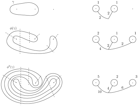
Figure 9: Left: the action on a curve $\gamma$ of an hyperbolic diffeomorphism $\phi$ on a punctured sphere $\Sigma_{0,4}$ (one puncture at infinity is not shown). Right: the corresponding train tracks, which count the thickness of the foldings of $\gamma$ along the dotted line under the iteration of the map.

Appendix B Hurwitz moves and ABC factorization

In this appendix we give some more details about the relation between our notation in section 5.1 and the more familiar F-theory approach in terms of moving branch cuts [91]. First, we reproduce in Table 2 the well known Kodaira list for the degeneration types of genus one curves.

Order	Singularity	Type	Monodromy
1	dbl. point	$I_{1}$	$V$
$n$	$A_{n-1}$	$I_{n}$	$V^{n}$
2	cusp	$II$	$UV$
3	$A_{1}$	$III$	$UVU$
4	$A_{2}$	$IV$	$(UV)^{2}$
6	$D_{4}$	$I_{0}^{\ast}$	$(UV)^{3}$
$6+n$	$D_{4+n}$	$I_{n}^{\ast}$	$(UV)^{3}V^{n}=-V^{n}$
8	$E_{6}$	$IV^{\ast}$	$(UV)^{4}=(UV)^{-2}$
9	$E_{7}$	$III^{\ast}$	$(UV)^{4}U=(UVU)^{-1}$
10	$E_{8}$	$II^{\ast}$	$(UV)^{5}=(UV)^{-1}$

Table 2: Kodaira classification of degenerations of elliptic fibers.

We give a factorization of the monodromy in terms of the two generators $U$, $V$ of the mapping class group of the fiber torus, corresponding to a Dehn twist along the $u$ cycle and a twist along the $v$ cycle, see Figure 1. Note that the starred types have a monodromy which is the inverse of the corresponding un-starred type. This follows trivially from the relations which present $SL(2,\mathbb{Z})$, namely from $(UV)^{6}=\mathbb{1}$ and from the braid relation $UVU=VUV$. We note that the degenerations of the table precisely correspond to parabolic elements (fibers $I_{n}$ and $I_{n}^{\ast}$) and to the elliptic conjugacy classes listed around (2.8). More precisely, all the mapping tori with parabolic and elliptic monodromies (where we restrict to a given chirality) arise at the boundary of small disks encircling the given degenerations, in line with the general theorem discussed in section 5.1.

Let us discuss now the Hurwitz moves on the above factorizations. We define elementary moves that consist in shifting the $V$ components one step from right to left. This gives $UV^{n}=VT_{n}$, where $T_{n}=V^{-n}UV^{n}$ (see Figure 10). Analogously, we get $VU^{n}=UT_{(-n)}$.

Figure 10: Elementary move.

Note that in terms of the more familiar ABC branes used in the F-theory literature (see for instance [108, 91, 109]), we have $V=A$, $T_{3}=B$ and $T_{1}=C$. We can use the elementary move on $V$ and the braid relation to bring the UV factorization in Table 2 to the corresponding ABC factorization. As an example, we show in Figure 11 the case for the $D_{4}$ singularity. From the braid relation (applied to the underlined twists) and the Hurwitz moves we obtain

$$\underline{UVU}VUV=VUVVUV=A^{4}BC\,,$$ (B.1)

which is the standard factorization for the $I_{0}^{\ast}$ monodromy. For the exceptional singularities we have (see Figure 12)

$$\underline{UVU}V\underline{UVU}V =VUVVVUVV=A^{6}BC\,,$$

$$\underline{UVU}V\underline{UVU}VU =VUVVVUVVU=A^{6}BC^{2}\,,$$

$$\underline{UVU}V\underline{UVU}VUV =VUVVVUVVUV\approx A^{7}BC\,,$$ (B.2)

where the last relation follows from a global $SL(2,\mathbb{Z})$ conjugation.

Figure 11: Hurwitz moves on the $I_{0}^{\ast}$ factorization.

Figure 12: Hurwitz moves on the monodromy factorizations for degenerations with exceptional singularities.

The UV factorization is useful to understand colliding singularities and the corresponding symmetry enhancements. For example, when two $III$ fibers collide we get a monodromy

$$III+III=UVU\,\underline{UVU}=UVU\,VUV=(UV)^{3}=I_{0}^{\ast}\,,$$ (B.3)

giving an $SO(8)$ gauge group. Another example is the branch II at constant $\tau$. There are generically twelve type $II$ degenerations, each with monodromy $UV$. To understand enhanced symmetries on this branch, we see that when $n$ singularities coincide, $n=(2,3,4,5)$, we get a monodromy $(UV)^{n}$, corresponding to the gauge groups $SU(3)$, $SO(8)$, $E_{6}$, $E_{8}$. This reproduces the list in [91].

Appendix C Geometry of torus fibrations

We summarize some details about the geometry of the ansatz (5.59). The relevant equations of motion are:

$$R-4(d\Phi)^{2}+4\nabla^{2}\Phi-\frac{1}{2}H^{2}=0\,,$$ (C.1)

$$R_{MN}+2\nabla_{M}\nabla_{N}\Phi-\frac{1}{2}\iota_{M}H\iota_{N}H=0\,,$$ (C.2)

$$d(e^{-2\Phi}\star_{10}H)=0\,.$$ (C.3)

It is easy to check that the Cauchy-Riemann equations for the functions $\tau$, $\rho$ and $\phi$ imply that the ansatz (5.59) solves the equations of motion. The Ricci scalar (in the string frame) for such ansatz is:

$$R=\frac{3e^{-2\varphi_{1}(r,\theta)}}{2r^{2}[\rho_{2}(r,\theta)]^{3}\tau_{2}(r,\theta)}\left[r^{2}\left(\frac{\partial\rho_{2}(r,\theta)}{\partial r}\right)^{2}+\left(\frac{\partial\rho_{2}(r,\theta)}{\partial\theta}\right)^{2}\right]\,.$$ (C.4)

For completeness we also give the components of the Ricci tensor along the torus and the base directions:

$$R_{r,r} =\frac{(1+\partial_{\theta}^{2}\varphi_{2})\partial_{r}\rho_{2}+\partial_{\theta}\rho_{2}\partial_{r}\varphi_{2}}{r\rho_{2}}+\frac{r^{2}\partial_{r}\rho_{2}\partial_{r}\tau_{2}-\partial_{\theta}\rho_{2}\partial_{\theta}\tau_{2}}{2r^{2}\rho_{2}\tau_{2}}+\frac{\partial_{\theta}^{2}\rho_{2}}{r^{2}\rho_{2}}+\frac{3(\partial_{r}\rho_{2})^{2}}{2\rho_{2}^{2}}\,,$$

$$R_{r,\theta} =\frac{\partial_{\theta}\rho_{2}(1+\partial_{\theta}\varphi_{2})}{r\rho_{2}}+\frac{3\partial_{\theta}\rho_{2}\partial_{r}\rho_{2}}{2\rho_{2}^{2}}+\frac{\partial_{\theta}\rho_{2}\partial_{r}\tau_{2}+\partial_{\theta}\tau_{2}\partial_{r}\rho_{2}}{2\rho_{2}\tau_{2}}-\frac{r\partial_{r}\rho_{2}\partial_{r}\varphi_{2}+\partial_{r}\partial_{\theta}\rho_{2}}{\rho_{2}}\,,$$

$$R_{\theta,\theta} =\frac{3(\partial_{\theta}\rho_{2})^{2}}{2\rho_{2}^{2}}-\frac{\partial_{\theta}^{2}\rho_{2}+r(1+\partial_{\theta}\varphi_{2})\partial_{r}\rho_{2}}{\rho_{2}}+\frac{\partial_{\theta}\rho_{2}\partial_{\theta}\tau_{2}-r^{2}\partial_{r}\rho_{2}\partial_{r}\tau_{2}}{2\rho_{2}\tau_{2}}-\frac{r\partial_{\theta}\rho_{2}\partial_{r}\varphi_{2}}{\rho_{2}}\,,$$

$$R_{8,8} =\frac{e^{-2\varphi_{1}}\tau_{1}}{r\rho_{2}\tau_{2}^{2}}\left[\partial_{\theta}\rho_{2}\partial_{r}\tau_{2}-\partial_{r}\rho_{2}\partial_{\theta}\tau_{2}\right]+\frac{e^{-2\varphi_{1}}(\tau_{1}^{2}-\tau_{2}^{2})}{2r^{2}\rho_{2}\tau_{2}^{3}}\left[\partial_{\theta}\rho_{2}\partial_{\theta}\tau_{2}+r^{2}\partial_{r}\rho_{2}\partial_{r}\tau_{2}\right]\,,$$

$$R_{8,9} =\frac{e^{-2\varphi_{1}}}{2r\rho_{2}\tau_{2}^{2}}\left[\partial_{\theta}\rho_{2}\partial_{r}\tau_{2}-\partial_{r}\rho_{2}\partial_{\theta}\tau_{2}\right]+\frac{e^{-2\varphi_{1}}\tau_{1}}{2r^{2}\rho_{2}\tau_{2}^{3}}\left[\partial_{\theta}\rho_{2}\partial_{\theta}\tau_{2}+r^{2}\partial_{r}\rho_{2}\partial_{r}\tau_{2}\right]\,,$$

$$R_{9,9} =\frac{e^{-2\varphi_{1}}}{2r^{2}\rho_{2}\tau_{2}^{3}}\left[\partial_{\theta}\rho_{2}\partial_{\theta}\tau_{2}+r^{2}\partial_{r}\rho_{2}\partial_{r}\tau_{2}\right]\,.$$ (C.5)

Appendix D T-duality

We recall well known facts about the action of an element of the T-duality group $O(2,2,\mathbb{Z})$ (see for example [110]). If we define the background matrix

$$E=G+B\,,$$ (D.1)

the action of an element

$$\Omega_{O(d,d)}=\begin{pmatrix}\mathbf{A}&\mathbf{B}\\ \mathbf{C}&\mathbf{D}\end{pmatrix}$$ (D.2)

on $E$ is

$$E\rightarrow\frac{\mathbf{A}E+\mathbf{B}}{\mathbf{C}E+\mathbf{D}}\,,$$ (D.3)

where the following relations hold:

$$\mathbf{A}^{T}\mathbf{C}+\mathbf{C}^{T}\mathbf{A}=\mathbf{B}^{T}\mathbf{D}+\mathbf{D}^{T}\mathbf{B}=0\,,\quad\mathbf{A}^{T}\mathbf{D}+\mathbf{C}^{T}\mathbf{B}=\mathbb{1}\,.$$ (D.4)

If we introduce the generalized matrix

$$M_{E}=\begin{pmatrix}G-BG^{-1}B&BG^{-1}\\ -G^{-1}B&G^{-1}\end{pmatrix}\,,$$ (D.5)

the action is $M_{E}\rightarrow\Omega M_{E}\Omega^{T}$. In terms of the $SL(2,\mathbb{Z})$ action on $\tau$ and $\rho$, defined as

$$\tau\rightarrow\frac{a\tau+b}{c\tau+d}\,,\qquad\rho\rightarrow\frac{\tilde{a}\rho+\tilde{b}}{\tilde{c}\rho+\tilde{d}}\,,\quad ad-bc=\tilde{a}\tilde{d}-\tilde{b}\tilde{c}=1\,,$$ (D.6)

the element $\Omega_{O(2,2)}$ is determined as follows:

$$\mathbf{A}=\tilde{a}\begin{pmatrix}a&b\\ c&d\end{pmatrix}\,,\quad\mathbf{B}=\tilde{b}\begin{pmatrix}-b&a\\ -d&c\end{pmatrix}\,,\quad\mathbf{C}=\tilde{c}\begin{pmatrix}-c&-d\\ a&b\end{pmatrix}\,,\quad\mathbf{D}=\tilde{d}\begin{pmatrix}d&-c\\ -b&a\end{pmatrix}\,.$$ (D.7)

In particular, the action of $SL(2,\mathbb{Z})_{\tau}$ is given by $O(2,2,\mathbb{Z})$ matrices of the form:

$$\Omega_{O(2,2),\tau}=\begin{pmatrix}M_{\tau}&0\\ 0&(M_{\tau}^{T})^{-1}\end{pmatrix}\,,$$ (D.8)

which is just a basis change $E\rightarrow M_{\tau}EM_{\tau}^{T}$. The action of $SL(2,\mathbb{Z})_{\rho}$ is embedded as

$$\Omega_{O(2,2),\rho}=\begin{pmatrix}\tilde{a}&\tilde{b}\,\omega\\ -\tilde{c}\,\omega&\tilde{d}\end{pmatrix}\,,$$ (D.9)

where $\omega=i\sigma_{2}=\bigl{(}\begin{smallmatrix}0&1\\ -1&0\end{smallmatrix}\bigr{)}$. Perturbative monodromies in $\rho$ given by the $SL(2,\mathbb{Z})$ element $V^{\tilde{b}}$ in (2.7), are identified with the upper right corner. We see then that upper triangular matrices represent a geometric subgroup $G_{geom}\subset O(2,2,\mathbb{Z})$ which is a product of diffeomorphisms and B-transformations of the form:

$$\Omega_{geom}=\begin{pmatrix}M_{\tau}&\tilde{b}\,M_{\tau}\cdot\omega\\ 0&(M_{\tau}^{T})^{-1}\end{pmatrix}\,.$$ (D.10)

A diffeomorphism combined with a $(0,1)$ element of the parabolic conjugacy classes in $SL(2,\mathbb{Z})_{\rho}$, namely $U^{\tilde{c}}$ (2.7) which acts as:

$$\rho\rightarrow\frac{\rho}{\tilde{c}\rho+1}\,,$$ (D.11)

is represented by a lower triangular matrix

$$\Omega_{\beta}=\begin{pmatrix}M_{\tau}&0\\ \tilde{c}\,\omega\cdot M_{\tau}&(M_{\tau}^{T})^{-1}\end{pmatrix}\,.$$ (D.12)

The action given by the transformation (D.11) forms an Abelian subgroup of $O(2,2,\mathbb{Z})$ usually referred to as $\beta$-transforms [18] since it acts naturally on bivectors $\beta\in\bigwedge^{2}TM$. Such elements implement TsT transformations and are very useful in holography to construct gravity duals of marginal deformations, such as $\beta$-deformations of $\mathcal{N}=4$ SYM [111, 112].

Other $SL(2,\mathbb{Z})_{\rho}$ transformations, such as the parabolic $(p,q)$ monodromy, will result in $O(2,2,\mathbb{Z})$ elements in which both B- and $\beta$-transformations are present at the same time.

References

- [1] E. Witten, “Geometric Langlands From Six Dimensions,” 0905.2720.
- [2] E. Witten, “Solutions of four-dimensional field theories via M theory,” Nucl.Phys. B500 (1997) 3–42, hep-th/9703166.
- [3] N. Halmagyi, C. Romelsberger, and N. P. Warner, “Inherited duality and quiver gauge theory,” Adv.Theor.Math.Phys. 10 (2006) 159–179, hep-th/0406143.
- [4] D. Gaiotto, “N=2 dualities,” JHEP 1208 (2012) 034, 0904.2715.
- [5] N. Seiberg and E. Witten, “Electric - magnetic duality, monopole condensation, and confinement in N=2 supersymmetric Yang-Mills theory,” Nucl. Phys. B426 (1994) 19–52, hep-th/9407087. [Erratum: Nucl. Phys.B430,485(1994)].
- [6] A. Klemm, W. Lerche, S. Yankielowicz, and S. Theisen, “Simple singularities and N=2 supersymmetric Yang-Mills theory,” Phys. Lett. B344 (1995) 169–175, hep-th/9411048.
- [7] A. Klemm, W. Lerche, P. Mayr, C. Vafa, and N. P. Warner, “Selfdual strings and N=2 supersymmetric field theory,” Nucl. Phys. B477 (1996) 746–766, hep-th/9604034.
- [8] C. Vafa, “Evidence for F theory,” Nucl.Phys. B469 (1996) 403–418, hep-th/9602022.
- [9] A. Kumar and C. Vafa, “U manifolds,” Phys.Lett. B396 (1997) 85–90, hep-th/9611007.
- [10] J. T. Liu and R. Minasian, “U-branes and T**3 fibrations,” Nucl.Phys. B510 (1998) 538–554, hep-th/9707125.
- [11] J. McOrist, D. R. Morrison, and S. Sethi, “Geometries, Non-Geometries, and Fluxes,” Adv.Theor.Math.Phys. 14 (2010) 1004.5447.
- [12] A. Malmendier and D. R. Morrison, “K3 surfaces, modular forms, and non-geometric heterotic compactifications,” 1406.4873.
- [13] J. Gu and H. Jockers, “Nongeometric F-theory–heterotic duality,” Phys.Rev. D91 (2015), no. 8 086007, 1412.5739.
- [14] B. R. Greene, A. D. Shapere, C. Vafa, and S.-T. Yau, “Stringy Cosmic Strings and Noncompact Calabi-Yau Manifolds,” Nucl.Phys. B337 (1990) 1.
- [15] S. Hellerman, J. McGreevy, and B. Williams, “Geometric constructions of nongeometric string theories,” JHEP 0401 (2004) 024, hep-th/0208174.
- [16] C. Hull, “A Geometry for non-geometric string backgrounds,” JHEP 0510 (2005) 065, hep-th/0406102.
- [17] N. Hitchin, “Generalized calabi-yau manifolds,” QUART.J.MATH.OXFORD SER. 54 (2003) 281.
- [18] M. Gualtieri, “Generalized complex geometry,” 2004.
- [19] W. Siegel, “Superspace duality in low-energy superstrings,” Phys. Rev. D48 (1993) 2826–2837, hep-th/9305073.
- [20] C. Hull and B. Zwiebach, “Double Field Theory,” JHEP 0909 (2009) 099, 0904.4664.
- [21] M. Grana, R. Minasian, M. Petrini, and D. Waldram, “T-duality, Generalized Geometry and Non-Geometric Backgrounds,” JHEP 04 (2009) 075, 0807.4527.
- [22] D. Andriot, O. Hohm, M. Larfors, D. Lüst, and P. Patalong, “Non-Geometric Fluxes in Supergravity and Double Field Theory,” Fortsch.Phys. 60 (2012) 1150–1186, 1204.1979.
- [23] D. Andriot and A. Betz, “Supersymmetry with non-geometric fluxes, or a -twist in Generalized Geometry and Dirac operator,” JHEP 1504 (2015) 006, 1411.6640.
- [24] F. Hassler and D. Lüst, “Consistent Compactification of Double Field Theory on Non-geometric Flux Backgrounds,” 1401.5068.
- [25] R. Blumenhagen, A. Deser, E. Plauschinn, F. Rennecke, and C. Schmid, “The Intriguing Structure of Non-geometric Frames in String Theory,” Fortsch.Phys. 61 (2013) 893–925, 1304.2784.
- [26] R. Blumenhagen, F. Hassler, and D. Lüst, “Double Field Theory on Group Manifolds,” JHEP 1502 (2015) 001, 1410.6374.
- [27] R. Blumenhagen, P. d. Bosque, F. Hassler, and D. Lüst, “Generalized Metric Formulation of Double Field Theory on Group Manifolds,” 1502.02428.
- [28] D. Andriot, M. Larfors, D. Lust, and P. Patalong, “A ten-dimensional action for non-geometric fluxes,” JHEP 09 (2011) 134, 1106.4015.
- [29] D. Andriot, O. Hohm, M. Larfors, D. Lust, and P. Patalong, “A geometric action for non-geometric fluxes,” Phys. Rev. Lett. 108 (2012) 261602, 1202.3060.
- [30] R. Blumenhagen, A. Deser, E. Plauschinn, and F. Rennecke, “Non-geometric strings, symplectic gravity and differential geometry of Lie algebroids,” JHEP 02 (2013) 122, 1211.0030.
- [31] R. Blumenhagen, A. Deser, E. Plauschinn, and F. Rennecke, “A bi-invariant Einstein-Hilbert action for the non-geometric string,” Phys. Lett. B720 (2013) 215–218, 1210.1591.
- [32] G. Aldazabal, D. Marques, and C. Nunez, “Double Field Theory: A Pedagogical Review,” Class.Quant.Grav. 30 (2013) 163001, 1305.1907.
- [33] O. Hohm, D. Lüst, and B. Zwiebach, “The Spacetime of Double Field Theory: Review, Remarks, and Outlook,” Fortsch.Phys. 61 (2013) 926–966, 1309.2977.
- [34] C. M. Hull, “Finite Gauge Transformations and Geometry in Double Field Theory,” 1406.7794.
- [35] K. Lee, C. Strickland-Constable, and D. Waldram, “New gaugings and non-geometry,” 1506.03457.
- [36] K. Kodaira, “On compact analytic surfaces i-iii,” Ann. of Math., 71 (1960), 111–152; 77 (1963), 563–626; 78 (1963), 1–40.
- [37] H. Ooguri and C. Vafa, “Two-dimensional black hole and singularities of CY manifolds,” Nucl.Phys. B463 (1996) 55–72, hep-th/9511164.
- [38] Y. Matsumoto and J. M. Montesinos-Amilibia, Pseudo-periodic Maps and Degeneration of Riemann Surfaces. Springer-Verlag, 2011.
- [39] A. Strominger, S.-T. Yau, and E. Zaslow, “Mirror symmetry is T duality,” Nucl.Phys. B479 (1996) 243–259, hep-th/9606040.
- [40] D. Vegh and J. McGreevy, “Semi-Flatland,” JHEP 0810 (2008) 068, 0808.1569.
- [41] K. Becker and S. Sethi, “Torsional Heterotic Geometries,” Nucl.Phys. B820 (2009) 1–31, 0903.3769.
- [42] J. de Boer and M. Shigemori, “Exotic Branes in String Theory,” Phys.Rept. 532 (2013) 65–118, 1209.6056.
- [43] F. Hassler and D. Lüst, “Non-commutative/non-associative IIA (IIB) Q- and R-branes and their intersections,” JHEP 1307 (2013) 048, 1303.1413.
- [44] A. Chatzistavrakidis, F. F. Gautason, G. Moutsopoulos, and M. Zagermann, “Effective actions of nongeometric five-branes,” Phys. Rev. D89 (2014), no. 6 066004, 1309.2653.
- [45] E. A. Bergshoeff, J. Hartong, T. Ortin, and D. Roest, “Seven-branes and Supersymmetry,” JHEP 0702 (2007) 003, hep-th/0612072.
- [46] C. Condeescu, I. Florakis, C. Kounnas, and D. Lüst, “Gauged supergravities and non-geometric Q/R-fluxes from asymmetric orbifold CFT‘s,” JHEP 1310 (2013) 057, 1307.0999.
- [47] P. Mayr and S. Stieberger, “Moduli dependence of one loop gauge couplings in (0,2) compactifications,” Phys. Lett. B355 (1995) 107–116, hep-th/9504129.
- [48] D. Andriot and A. Betz, “NS-branes, source corrected Bianchi identities, and more on backgrounds with non-geometric fluxes,” JHEP 07 (2014) 059, 1402.5972.
- [49] M. Park and M. Shigemori, “Condimension-2 Solutions in Five-Dimensional Supergravity,” 1505.05169.
- [50] T. Damour, M. Henneaux, and H. Nicolai, “Cosmological billiards,” Class.Quant.Grav. 20 (2003) R145–R200, hep-th/0212256.
- [51] J. Brown, O. J. Ganor, and C. Helfgott, “M theory and E(10): Billiards, branes, and imaginary roots,” JHEP 0408 (2004) 063, hep-th/0401053.
- [52] X. Dong, B. Horn, E. Silverstein, and G. Torroba, “Micromanaging de Sitter holography,” Class.Quant.Grav. 27 (2010) 245020, 1005.5403.
- [53] C. Nayak, S. H. Simon, A. Stern, M. Freedman, and S. Das Sarma, “Non-Abelian anyons and topological quantum computation,” Reviews of Modern Physics 80 (July, 2008) 1083–1159, 0707.1889.
- [54] A. Lerda and S. Sciuto, “Anyons and quantum groups,” Nucl. Phys. B401 (1993) 613–643, hep-th/9301100.
- [55] A. Dabholkar and C. Hull, “Duality twists, orbifolds, and fluxes,” JHEP 0309 (2003) 054, hep-th/0210209.
- [56] C. Hull and R. Reid-Edwards, “Flux compactifications of string theory on twisted tori,” Fortsch.Phys. 57 (2009) 862–894, hep-th/0503114.
- [57] B. Wecht, “Lectures on Nongeometric Flux Compactifications,” Class.Quant.Grav. 24 (2007) S773–S794, 0708.3984.
- [58] M. Graña, R. Minasian, H. Triendl, and T. Van Riet, “Quantization problem in Scherk-Schwarz compactifications,” Phys.Rev. D88 (2013), no. 8 085018, 1305.0785.
- [59] R. Benedetti and C. Petronio, Lectures on Hyperbolic Geometry. Springer-Verlag, 1992.
- [60] O. DeWolfe, T. Hauer, A. Iqbal, and B. Zwiebach, “Uncovering infinite symmetries on [p, q] 7-branes: Kac-Moody algebras and beyond,” Adv.Theor.Math.Phys. 3 (1999) 1835–1891, hep-th/9812209.
- [61] P. Scott, “The geometries of 3-manifolds,” Bull. London Math. Soc. 15 (5) (1983) 401–487.
- [62] C. Hull, “Global aspects of T-duality, gauged sigma models and T-folds,” JHEP 0710 (2007) 057, hep-th/0604178.
- [63] C. M. Hull and R. A. Reid-Edwards, “Flux compactifications of M-theory on twisted Tori,” JHEP 10 (2006) 086, hep-th/0603094.
- [64] C. M. Hull and R. A. Reid-Edwards, “Gauge symmetry, T-duality and doubled geometry,” JHEP 08 (2008) 043, 0711.4818.
- [65] C. M. Hull and R. A. Reid-Edwards, “Non-geometric backgrounds, doubled geometry and generalised T-duality,” JHEP 09 (2009) 014, 0902.4032.
- [66] S. Kachru, M. B. Schulz, P. K. Tripathy, and S. P. Trivedi, “New supersymmetric string compactifications,” JHEP 0303 (2003) 061, hep-th/0211182.
- [67] J. Shelton, W. Taylor, and B. Wecht, “Nongeometric flux compactifications,” JHEP 0510 (2005) 085, hep-th/0508133.
- [68] D. M. Belov, C. M. Hull, and R. Minasian, “T-duality, gerbes and loop spaces,” 0710.5151.
- [69] E. Plauschinn, “On T-duality transformations for the three-sphere,” Nucl.Phys. B893 (2015) 257–286, 1408.1715.
- [70] M. Grana, R. Minasian, M. Petrini, and A. Tomasiello, “A scan for new N=1 vacua on twisted tori,” JHEP 05 (2007) 031, hep-th/0609124. [hep-th/0609124].
- [71] E. Silverstein, “Simple de Sitter Solutions,” Phys.Rev. D77 (2008) 106006, 0712.1196.
- [72] F. Hassler, D. Lüst, and S. Massai, “On Inflation and de Sitter in Non-Geometric String Backgrounds,” 1405.2325.
- [73] C. Condeescu, I. Florakis, and D. Lüst, “Asymmetric Orbifolds, Non-Geometric Fluxes and Non-Commutativity in Closed String Theory,” JHEP 1204 (2012) 121, 1202.6366.
- [74] C. M. Hull, “Massive string theories from M theory and F theory,” JHEP 11 (1998) 027, hep-th/9811021.
- [75] I. Ellwood and A. Hashimoto, “Effective descriptions of branes on non-geometric tori,” JHEP 12 (2006) 025, hep-th/0607135.
- [76] W. Schulgin and J. Troost, “Backreacted T-folds and non-geometric regions in configuration space,” JHEP 0812 (2008) 098, 0808.1345.
- [77] O. DeWolfe, T. Hauer, A. Iqbal, and B. Zwiebach, “Uncovering the symmetries on [p,q] seven-branes: Beyond the Kodaira classification,” Adv.Theor.Math.Phys. 3 (1999) 1785–1833, hep-th/9812028.
- [78] Y. Namikawa and K. Ueno, “The complete classification of fibres in pencils of curves of genus two,” manuscripta mathematica 9 (1973), no. 2 143–186.
- [79] J. de Boer and M. Shigemori, “Exotic branes and non-geometric backgrounds,” Phys.Rev.Lett. 104 (2010) 251603, 1004.2521.
- [80] N. Obers and B. Pioline, “U duality and M theory,” Phys.Rept. 318 (1999) 113–225, hep-th/9809039.
- [81] M. Blau and M. O’Loughlin, “Aspects of U duality in matrix theory,” Nucl. Phys. B525 (1998) 182–214, hep-th/9712047.
- [82] E. Lozano-Tellechea and T. Ortin, “7-branes and higher Kaluza-Klein branes,” Nucl. Phys. B607 (2001) 213–236, hep-th/0012051.
- [83] J. de Boer, D. R. Mayerson, and M. Shigemori, “Classifying Supersymmetric Solutions in 3D Maximal Supergravity,” Class. Quant. Grav. 31 (2014), no. 23 235004, 1403.4600.
- [84] J. Raeymaekers and D. Van den Bleeken, “Unlocking the Axion-Dilaton in 5D Supergravity,” JHEP 1411 (2014) 029, 1407.5330.
- [85] T. Kikuchi, T. Okada, and Y. Sakatani, “Rotating string in doubled geometry with generalized isometries,” Phys. Rev. D86 (2012) 046001, 1205.5549.
- [86] E. A. Bergshoeff and F. Riccioni, “D-Brane Wess-Zumino Terms and U-Duality,” JHEP 11 (2010) 139, 1009.4657.
- [87] E. A. Bergshoeff and F. Riccioni, “String Solitons and T-duality,” JHEP 05 (2011) 131, 1102.0934.
- [88] E. A. Bergshoeff, T. Ortin, and F. Riccioni, “Defect Branes,” Nucl. Phys. B856 (2012) 210–227, 1109.4484.
- [89] D. Auroux, “Mapping class group factorizations and symplectic 4-manifolds: some open problems,” Proc. Symp. Pure Math. 74 (2006) 123–132.
- [90] F. Catanese, “Trecce, Mapping class group, fibrazioni di Lefschetz ed applicazioni al diffeomorfismo di superficie algebriche,” ArXiv Mathematics e-prints (May, 2004) math/0405300.
- [91] M. R. Gaberdiel, T. Hauer, and B. Zwiebach, “Open string-string junction transitions,” Nucl.Phys. B525 (1998) 117–145, hep-th/9801205.
- [92] H. Ooguri and C. Vafa, “Summing up D instantons,” Phys.Rev.Lett. 77 (1996) 3296–3298, hep-th/9608079.
- [93] T. W. Grimm, D. Klevers, and M. Poretschkin, “Fluxes and Warping for Gauge Couplings in F-theory,” JHEP 01 (2013) 023, 1202.0285.
- [94] C. V. Johnson, A. W. Peet, and J. Polchinski, “Gauge theory and the excision of repulson singularities,” Phys.Rev. D61 (2000) 086001, hep-th/9911161.
- [95] R. Gregory, J. A. Harvey, and G. W. Moore, “Unwinding strings and t duality of Kaluza-Klein and h monopoles,” Adv.Theor.Math.Phys. 1 (1997) 283–297, hep-th/9708086.
- [96] D. Tong, “NS5-branes, T duality and world sheet instantons,” JHEP 0207 (2002) 013, hep-th/0204186.
- [97] J. McOrist and S. Sethi, “M-theory and Type IIA Flux Compactifications,” JHEP 12 (2012) 122, 1208.0261.
- [98] T. Ashikaga and K. Konno, “Global and local properties of pencils of algebraic curves,” in Algebraic Geometry 2000, Azumino, Adv. Stud. in Pure Math, pp. 1–49.
- [99] L. Martucci, J. F. Morales, and D. R. Pacifici, “Branes, U-folds and hyperelliptic fibrations,” JHEP 01 (2013) 145, 1207.6120.
- [100] A. P. Braun, F. Fucito, and J. F. Morales, “U-folds as K3 fibrations,” JHEP 1310 (2013) 154, 1308.0553.
- [101] P. Candelas, A. Constantin, C. Damian, M. Larfors, and J. F. Morales, “Type IIB flux vacua from G-theory I,” JHEP 02 (2015) 187, 1411.4785.
- [102] P. Candelas, A. Constantin, C. Damian, M. Larfors, and J. F. Morales, “Type IIB flux vacua from G-theory II,” JHEP 02 (2015) 188, 1411.4786.
- [103] R. Blumenhagen, D. Lüst, and S. Theisen, Basic Concepts of String Theory. Springer-Verlag Berlin Heidelberg, 2013.
- [104] B. Farb and D. Margalit, A Primer on Mapping Class Groups. Princeton University Press, 2011.
- [105] R. Blumenhagen and R. Sun, “T-duality, Non-geometry and Lie Algebroids in Heterotic Double Field Theory,” JHEP 02 (2015) 097, 1411.3167.
- [106] M. Bianchi, G. Pradisi, C. Timirgaziu, and L. Tripodi, “Heterotic T-folds with a small number of neutral moduli,” JHEP 10 (2012) 089, 1207.2665.
- [107] A. Font, I. García-Etxebarria, D. Lüst, S. Massai, and C. Mayrhofer, “to appear,”.
- [108] A. Johansen, “A Comment on BPS states in F theory in eight-dimensions,” Phys. Lett. B395 (1997) 36–41, hep-th/9608186.
- [109] R. Blumenhagen, “Basics of F-theory from the Type IIB Perspective,” Fortsch.Phys. 58 (2010) 820–826, 1002.2836.
- [110] A. Giveon, M. Porrati, and E. Rabinovici, “Target space duality in string theory,” Phys.Rept. 244 (1994) 77–202, hep-th/9401139.
- [111] O. Lunin and J. M. Maldacena, “Deforming field theories with U(1) x U(1) global symmetry and their gravity duals,” JHEP 0505 (2005) 033, hep-th/0502086.
- [112] R. Minasian, M. Petrini, and A. Zaffaroni, “Gravity duals to deformed SYM theories and Generalized Complex Geometry,” JHEP 0612 (2006) 055, hep-th/0606257.