Socially Constrained Structural Learning for Groups Detection in Crowd

Abstract

Modern crowd theories agree that collective behavior is the result of the underlying interactions among small groups of individuals. In this work, we propose a novel algorithm for detecting social groups in crowds by means of a Correlation Clustering procedure on people trajectories. The affinity between crowd members is learned through an online formulation of the Structural SVM framework and a set of specifically designed features characterizing both their physical and social identity, inspired by Proxemic theory, Granger causality, DTW and Heat-maps. To adhere to sociological observations, we introduce a loss function ($G$-MITRE) able to deal with the complexity of evaluating group detection performances. We show our algorithm achieves state-of-the-art results when relying on both ground truth trajectories and tracklets previously extracted by available detector/tracker systems.

1 Introduction

Crowd phenomena are complex and their logic still escapes formal rules and precise social explanations. Eventually, the ambition of crowd analysis is to characterize people behaviors, predict and prevent potentially dangerous situations and improve the well-being of communities. This has been traditionally provided by simulation models [1] or automatic video analysis [2]. Recently, groups have been recognized as the basic elements which compose the crowd [3], leading to an intermediate level of abstraction that is placed between two outfacing views: the crowd as a flow of indistinguishable people [4] and its interpretation as a collection of individuals [5]. Identifying groups is consequently a mandatory step to grasp the complex social dynamics ruling collective behaviors in crowds. This poses new challenges for computer vision, since groups are definitely more difficult to characterize than pedestrians acting alone or as a whole.

In this work, we propose a learning based solution for visually detecting groups in low/medium density crowds (Fig. 1) under the hypothesis that the concept of group can be visually discerned and people trajectories can be extracted up to some extent. The strong novelty of our approach is the joint adoption of sociologically grounded features and a learning framework able to specialize the concept of group accounting for different scenarios, motion constraints and crowd densities. To this end, we adhere to a classical sociological interpretation of groups [6], which can be formalized as follows.

Definition 1.

A group is defined as two or more people interacting to reach a common goal and perceiving a shared membership, based on both physical and social identity.

Accordingly, we propose a new formulation of the problem of detecting groups in crowds as a supervised Correlation Clustering (CC) [7]. We solve it through a Structural Support Vector Machines (Structural SVM) [8] framework that learns a context dependent distance measure, based on a set of features inspired by Def. 1 effective on both ground truth trajectories and automatically obtained tracklets. The design of socially grounded features is one of the main contributions of the work.

(a) student003

(b) 1shatian3

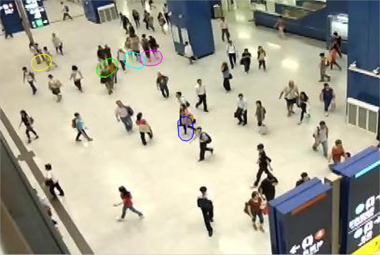
(c) 1dawei1

Figure 1: Examples of social groups detected in crowds.

Moreover, a new socially based loss function ($G$-MITRE) is defined for the Structural SVM. Differently from previous solutions [9] and [2], our approach doesn’t rely on scene-dependent parameters that would limit the applicability of the method in real world contexts. Finally, we also propose an online learning procedure that handles smooth variation in crowd composition and density, useful in online surveillance.

We annotated and made publicly available two new datasets: MPT-${\bf 20}$x${\bf 100}$ and GVEII (see Sec. 7). Results on standard benchmarks, as well as on the proposed datasets, outperform current methods. We strongly believe that an automatic system for group detection will influence future public area visual surveillance and will bring benefits to modeling and simulation application for architectural planning by providing real and precise data observation of crowds phenomena.

2 Related Work

The modeling of pedestrian dynamics in crowds represents a relatively recent research field. Most of the works are based on sociological paradigms and computer vision based approaches have also evolved under the influence of these theories.

Modeling and Observing the Crowd

Most of the research work has tried to tackle the crowd as an exclusively collective phenomenon, where individuality does not exist. This recalls the primitive Popular Mind Theory [10] by Gustave Le Bon, where the crowd was defined as a “pathological monster with no individual consciousness”. Accordingly, crowds have been analyzed by means of physical models (e.g. hydrodynamics [4]), neglecting the existence of single individual purposes and goals. However, these models are effective mainly in extremely dense crowds. Conversely, many other approaches have been inspired by the 70s Social Loafing Theory [11], which stated that individuality was a strong requirement for the pursuit of personal goals. Helbings Social Force Model [5], which asserts that anyone movements towards her goals are influenced by the surrounding pedestrians, has been the main building block for many crowd modeling and analysis works, ranging from abnormal behavior detection [12] to tracking [13]. Recently, studies on people attending events have underlined that most of the people tend to move in groups and social relations influence the way people behave in crowds [3, 14]. These empirical observations are supported by Reicher in the recent Social Identity Model of Deindividuation Effects [15], which assumes that crowd behavior is regulated by the social rules and behaviors groups choose to adopt. This is the main social paradigm underpinning our research too.

Visual Detection of Groups in Crowds

It was only recently that group detection showed promising results. The process is in fact built upon several open challenges in computer vision, starting from people detection and tracking in crowds [16] to analyzing and grouping extracted trajectories [17].

Some works employ the concept of F-formations by Kendon [18] to discern group formation process. Broadly speaking, F-formations can be seen as specific positional and orientational patterns that people must sustain in order to be considered engaged in a social relationship. Despite robust results [19], this theory is suited to stationary groups only and is not defined for moving groups, a case which cannot be ignored in crowd analysis.

Thus, complementary approaches analyze pedestrians motion paths; according to the type of available tracklets, they can be partitioned in group-based, individual-group joint and individual-based. In group-based approaches, groups are considered as atomic entities in the scene since no higher level information can be extracted neatly, typically due to high noise or high complexity of crowded scenes [20, 21]. Since these models are often too simplistic to further infer on groups behavior, individual-group joint approaches try to overcome the lack of finer information by hypothesizing trajectories while tracking groups at a coarser level [22, 23]. Finally, individual-based tracking algorithms build up on single pedestrians trajectories. This kind of approach has been gaining momentum only recently since tracking even in high density crowds is becoming everyday a more feasible task [16]. Pellegrini et al. [9] employ a Conditional Random Field to jointly predict trajectories and estimate group memberships, modeled as latent variables, over a short time window. Yamaguchi et al. [24] predict whether two pedestrians are in the same group through a linear SVM on trivial distance, speed difference and time overlap information. Recently, Chang et al. [25] proposed a soft segmentation process to partition the crowd by constructing a weighted graph, where the edges represent the probability of individuals to belong to the same group. An interesting unsupervised approach is Zanotto et. al  [26], where a potentially infinite mixture model is fitted on pedestrians, regarded as sampled observations from the mixture. Previous frames data and predictions are used as prior information for the models (one for each group), but pairwise relations between individuals are neglected as groups are modeled only through the mean position and velocity of their members. Above all, we mention Ge et al. [2] that suggests the use of an agglomerative approach to cluster trajectories, as we do. They hierarchically merge clusters by evaluating a well-founded sociological inter-group closeness measure defined on a combination of proximity and velocity features, stopping when a given condition is met.

Conversely, our method does not rely neither on relative position or velocity fixed thresholds [2, 26] nor on sequence-dependent parameters [9]; it is flexible and general as the features are not scene-specific [25] and their contribution is learned from examples. Thanks to the use of a clustering inference rule, solutions proposed by our method are partitions and not coverings of the members of the crowd [24], meaning that pairwise relations are consistent with the overall group structure found. Moreover, the use of a time window to predict groups let the method recognize that non-trivial behaviors (e.g. neglecting strict proximity) may occur, whereas frame-by-frame methods are limited to short term reasoning [26]. Yet, the discriminative nature of the employed framework makes learning compelling in terms of both required data and computational cost, as opposed to graphical models optimizing over a multiple hypothesis space [9].

This work extends our preliminary attempt in [17]. Here we prove our proposal complies with social theories of group formation, we devise and investigate new features to better adhere to the sociological theory underpinning our method and, eventually, extend the tests to new remarkably complex datasets and compare with more recent competing algorithms. Besides, the experiments further probe the need for learning when dealing with heterogeneous crowds, shedding light on the nature of the problem itself.

3 Problem Definition

We cast the group detection task as a clustering problem. Consider a set of pedestrian $M=\{a,b,\dots\}$ and $\mathcal{Y}(M)$ as the set of all possible ways to partition $M$. Defining $y$ as a subset of pedestrians (also referred to as group or cluster) in $M$, a generic set of subsets ${\bf y}~{}=~{}\{y_{1},y_{2},\dots\}$ is a valid solution in $\mathcal{Y}(M)$ if the partitioning axioms are satisfied: $\forall a\in\mathcal{M},\exists!y\in\mathcal{Y}(\mathcal{M}):a\in y$ and $\cup_{y\in\mathcal{Y}(\mathcal{M})}y=\mathcal{M}$. Here, we call singletons those pedestrians whose cluster is composed by themselves only, i.e. $|y|=1$.

In crowded contexts, this grouping cannot be solved by exploiting spatial (positional or orientational) information only, as proposed in F-formation theory, due both to confusion and motion. Moreover, it is often the case that the physical distance between a singleton and a member of a cluster is lower than that cluster intra-member mean distance. This is due to the fact that, in real situations, social aspects heavily intervene in the group formation process. In order to obtain crowd partitions that are meaningful from a sociological point of view, the following relevant properties of social groups must hold.

Hierarchical Coherence. Groups are composed by individuals and sub-groups in a recursive fashion (Fig.2a). This has been first observed in the seminal work of Canetti [27], based on the assumption that members within a group cannot erase already settled relationships as the crowd assembles.

Density Invariance. To keep their group identities preserved at different crowd densities, members must be willing to change the inner distance among them. Groups in very crowded scenes will be more closed and compact, while groups in open spaces will tend to exhibit more dilated patterns (Fig. 2b); sociologically and empirical evidence can be found in Bandini et al. [14] and in Moussaid et al. [3].

Transitivity. Not every member of a group needs to be strictly connected with every one else, but any two members may be part of the same group by means of a sufficiently dense subgroup of pedestrian standing between them (Fig. 2c). McPhail and Wohlstein’s work [28] formalized this idea: to be considered part of a group one typically will have to be connected with at least half of the members.

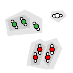
(a)

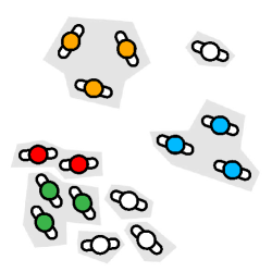
(b)

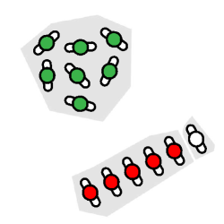
(c)

Figure 2: Highlights of social groups properties: (a) hierarchical coherence, (b) density invariance and (c) transitivity.

4 Socially Constrained Clustering for Groups Detection

We propose to solve the crowd partitioning problem employing the Correlation Clustering (CC) [7] and we prove it is possible to achieve a quasi-optimal crowd partition guaranteed to satisfy the three aforementioned properties of Sec. 3. The CC algorithm takes as input an affinity matrix $W$ where, if $W^{ab}>0$ ($W^{ab}<0$), elements $a$ and $b$ belong to the same (different) cluster with certainty $|W^{ab}|$. The algorithm returns the partition ${\bf y}$ of a set of elements $M=\{a,b,\dots\}$ so that the sum of the affinities between item pairs in the same clusters $y$ is maximized:

$$\text{CC}=\arg\max_{{\bf y}\in\mathcal{Y}(M)}\sum_{y\in{\bf y}}\sum_{a\neq b\in y}W^{ab}_{\bf d}.$$ (1)

The pairwise elements affinity in $W$ is parameterized as weighted linear combination of a bounded dissimilarity measure and its complement:

$$W^{ab}_{\bf d}={\boldsymbol{\alpha}}^{T}({\bf 1}-{\bf d}(a,b))-{\boldsymbol{\beta}}^{T}{\bf d}(a,b).$$ (2)

To be consistent with the definition of groups of Sec. 1, we devise the pairwise distance between pedestrian $a$ and $b$, ${\bf d}(a,b)$ as detailed in Sec. 5.

In clustering theory, changing the dissimilarity space results in different partitioning of the domain through the same algorithm. By tuning $[{\boldsymbol{\alpha}},{\boldsymbol{\beta}}]$ parameters in Eq. (2) we can evaluate many different groupings and we’ll show that, under a restrict set of hypothesis, they all satisfy the social properties previously mentioned. In order to efficiently learn those parameters according to different peculiarities groups exhibit in different scenarios, in Sec. 6 we introduce Structural SVM [29] with both an approximated inference procedure and a loss function specifically designed for accurately measuring the compatibility among possible crowd partitions.
The solution to Eq. (1), given the parametrization introduced in Eq. (2) and subject to a hierarchical inference procedure, guarantees the satisfaction of all the social groups properties:

Theorem 1.

When the pairwise elements affinity in $W$ is a weighted linear combination of a bounded similarity measure and its complement, a bottom-up approximated solution to CC produces a partition that respects the hierarchical coherence, density invariance and transitivity properties of social groups.

Proof.

Let ${\bf d}:M\times M\rightarrow[0,1]^{p}$ be a bounded distance on the set of members of a crowd $M$ so that $(M,{\bf d})$ is a dissimilarity space and suppose the affinity matrix of CC is constructed as in Eq. (2), for some appropriate positive values of ${\boldsymbol{\alpha}},{\boldsymbol{\beta}}\in\mathbb{R}^{p}$. To demonstrate that the density invariance holds for all solutions of CC consider that when the density increases, both distances between groups and between members of the same group diminish. This phenomenon is a less formal statement of the scale invariance axiom of clustering defined in Kleiberg [30] which is known to hold for sum-of-pairs clustering algorithm. We must thus show that it holds when we are maximizing affinities instead of minimizing distances as well. To this aim let ${\bf d}=\lambda\bar{\bf d}$ and $\bar{\bf d}:M\times M\rightarrow[0,\frac{1}{\lambda}]^{p}$ so that

$$W_{\bf d} ={\boldsymbol{\alpha}}^{T}({\bf 1}-\lambda\bar{\bf d})-{\boldsymbol{\beta}}^{T}\lambda\bar{\bf d}$$ (3)

$$=\lambda[{\boldsymbol{\alpha}}^{T}(\frac{1}{\lambda}-\bar{\bf d})-{\boldsymbol{\beta}}^{T}\bar{\bf d}]=\lambda W_{\bar{\bf d}},$$

where the notation for the elements is dropped for clarity. Consequently, CC satisfies the scale invariance axiom since multiplying all distances by a constant results in multiplying the total affinity of each cluster by a constant and hence the maximum affinity clustering solution is not changed. Transitivity follows directly from the objective function of CC in Eq. (1): to be assigned to the same group it suffices the existence of any number of members such that the net effect of all the involved pairwise relations is non-decreasing. Last, the hierarchical coherence requires a greedy approximation algorithm to optimize the CC that initially consider each pedestrian in its own cluster and then iteratively merges the two clusters whose union would produce the best clustering score, stopping when joining clusters would decrease the overall affinity. Hence, elements in the same cluster at lower levels of the hierarchy are also together in higher level clusters. ∎

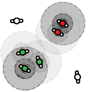
(a) Physical distance

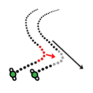
(b) Motion causality

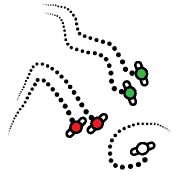
(c) Trajectory shape

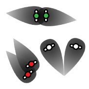
(d) Paths convergence

Figure 3: Features: physical identity (a) and social identity (b,c) provide a computational interpretation of the concept of group membership, while (d) evaluates the likeliness of the existence of a shared goal between pedestrians.

5 Social Features for Social Groups

Given the problem formulation in Sec. 3 and the CC parametrization of Eq. (2), here we define the distance function ${\bf d}$ which acts on trajectories pairs. We consider the pedestrian trajectory $T_{a}=\{(t,{\bf p}_{a}^{t})\}_{t}$, projected onto the ground plane, as multivariate time series of metric (in meters) spatial observations ${\bf p}_{a}^{t}$ for pedestrian $a$ at different times $t$. In order to deal with the continuously changing nature of groups (splitting, merging, switching members, $\dots$) we reduce the observation period to a time window $\mathcal{T}$ of fixed length. As a consequence, groups can be differently detected even between (potentially overlapped) sequential time windows $\mathcal{T}_{k}$ and $\mathcal{T}_{k+1}$.

According to Def. 1, we devise four features able to capture both the pedestrian physical and social identity as well as to discern the presence of a shared goal among them, namely: physical identity $d_{\text{ph}}$, trajectories shape-similarity $d_{\text{sh}}$, pedestrians causality $d_{\text{ca}}$ and heat-maps $d_{\text{hm}}$. A pairwise feature vector ${\bf d}^{k}(a,b)$ is hence defined for every couple of trajectories $T_{a}$ and $T_{b}$ and for every time window $\mathcal{T}_{k}$, as

$${\bf d}(a,b)\stackrel{{\scriptstyle\text{\tiny def}}}{{=}}{\bf d}^{k}(a,b)=[d_{\text{ph}},d_{\text{sh}},d_{\text{ca}},d_{\text{he}}]_{a,b}^{k}.$$ (4)

5.1 From Physical Distances to Physical Identity

(a)

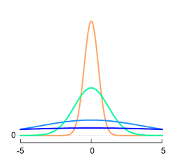
(b)

Figure 4: Proxemics, modeled by gaussians (b), reveal physical identity trough physical distance (a).

The physical identity can be regarded as a static relation connecting physical distance to group membership. In his Proxemic Theory, Hall [31] focused on the physical interactions between pairs of individuals. More precisely, the theory is about “the study of ways in which man gains knowledge of the content of other men’s minds through judgments of behaviour patterns associated with varying degrees of proximity to them.”

TABLE I: Proxemics characterization as found in Hall’s Theory.

space	boundaries ($m$)	description
intimate	0.0 - 0.5	unmistakable involvement
personal	0.5 - 1.2	familiar interactions
social	1.2 - 3.7	formal relationships
public	3.7 - 7.6	non-personal interactions

The proxemic model fomalizes how people use physical space in interpersonal interactions and defines a set of concentric bubbles around every individual, as depicted in Fig. 3a. Nevertheless, the transition between the four different proxemic zones is abrupt (Tab. I).

Spatial quantization can be heavily affected by noise or errors, leading to wrong classification. Several approaches assign a score to proxemic classes in order to obtain a continuous real-valued similarity measure, [32, 33, 1]. To grasp the distance based characteristics of group formation, we relax the original Hall’s quantization by employing a Gaussian Mixture Model (GMM) on the ground plane, centered on person location and with fixed proxemics-inspired covariance matrices. The resulting GMM is a weighted sum of zero mean Gaussians with diagonal covariance matrices reflecting Hall’s boundaries (i.e. $\Sigma_{1}\leftarrow 0.5$, $\Sigma_{2}\leftarrow 1.2$, …):

$$\text{GMM}({\bf p}_{a}^{t}-{\bf p}_{b}^{t})=\frac{1}{4}\sum\limits_{z=1}^{4}\mathcal{N}({\bf p}_{a}^{t}-{\bf p}_{b}^{t}|0,\Sigma_{z})$$ (5)

Given a pair of trajectories $T_{a}$ and $T_{b}$ we evaluate the mixture model of Eq. (5) on the vector of distances at each time instance. This is equivalent to place the mixture on ${\bf p}_{a}^{t}$ and measure where the point ${\bf p}_{b}^{t}$ lies inside the proxemic space at each instant $t$, as shown in Fig. 4 and in Fig. LABEL:fig:prox2.

The static measure of social cohesion, called $d_{\text{ph}}$, is then defined by averaging the mixture model responses over the the set of time instances where trajectories $T_{a}$ and $T_{b}$ are simultaneously present in the current time window, $\overline{\mathcal{T}}\subseteq\mathcal{T}^{k}$:

$$d_{\text{ph}}^{k}(a,b)=\frac{1}{|\overline{\mathcal{T}}|}\sum_{t\in\overline{\mathcal{T}}}\text{GMM}({\bf p}_{a}^{t}-{\bf p}_{b}^{t})$$ (6)

Averaging is required since the physical identity among group members is established in time and must remain coherent in order to be a valid measure of social cohesion.

5.2 Motion as an Indicator of Social Identity

Social Identity [34, 6] is a psychological paradigm built on the intuition that group behavior is an emerging dynamic, reflecting a shift in self-conception of the members who start to define themselves in terms of their common membership. According to [35], social identity reflects in the way people mutually influence each other and consequently move in groups, suggesting that social identity could be observed through trajectories shape similarity and paths temporal causality.

5.2.1 Temporal Causality

Under the hypothesis of sufficiently stationary trajectories, which is typically true for the observation of a time window, we can employ the econometric model of Granger causality [36] to measure to what extent pedestrians are mutually affecting their motion paths [37]. Accordingly, we formalize two requirements:

1. the causal pedestrian will move before the effect pedestrian, and

2. the motion of the causal pedestrian contains information about the way the effect pedestrian moves that cannot be found in any other pedestrian motion.

A consequence of these statements is that the causal pedestrian trajectory can help forecast the effect pedestrian trajectory even after other data has first been used. Let’s define $m$ as the lag value for the causality analysis and denote the optimum least-squares predictor of a stationary trajectory $T_{a}$ at time $t$ using the set of values $\bar{T}_{a}(t-m)$ by $P_{t}(T_{a}|\bar{T}_{a}(t-m))$. Here $\bar{T}_{a}(t-m)$ is all the information about trajectory $T_{a}$ accumulated since time $t-m$ (inside the current time window $\mathcal{T}^{k}$) up to time $t-1$. The predictive error series will be denoted by $\varepsilon_{t}(T_{a}|\bar{T}_{a}(t-m))=T_{a}(t)-P_{t}(T_{a}|\bar{T}_{a}(t-m))$ and define $\sigma^{2}(T_{a}|\bar{T}_{a}(t-m))$ as the variance of $\varepsilon_{t}(T_{a}|\bar{T}_{a}(t-m))$. It is said trajectory $T_{b}$ Granger causes $T_{a}$, briefly $b\rightarrow a$, if

$$\sigma^{2}(T_{a}|\bar{T}_{a}(t-m))>\sigma^{2}(T_{a}|\bar{T}_{a}(t-m),\bar{T}_{b}(t-m))$$ (7)

The feature is then derived from a specific testing procedure used to evaluate Granger causality trustworthiness. Let’s introduce the sum of squared residuals for the constrained and unconstrained models as

$$RSS_{c} =\sum_{t=1}^{K}\varepsilon_{t}(T_{a}|\bar{T}_{a}(t-m))^{2}\quad\text{and}\quad$$ (8)

$$RSS_{u} =\sum_{t=1}^{K}\varepsilon_{t}(T_{a}|\bar{T}_{a}(t-m),\bar{T}_{b}(t-m))^{2},$$

where $K$ is the number of samples considered for the analysis.

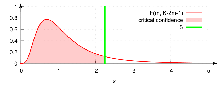
Figure 5: Visual example of causality probability. The vertical line is the $S$ of Eq. (9) while the shaded area is $d_{\text{ca}}$.

We design our feature $d_{\text{ca}}$ so as to be the critical confidence measure of the hypothesis that Granger causality exists between $T_{a}$ and $T_{b}$. To this end, we consider the test statistic

$$S_{b\rightarrow a}=\frac{(RSS_{c}-RSS_{u})/m}{RSS_{u}/(K-2m-1)}.$$ (9)

and compute the area under the Fisher-Snedecor probability function $\mathcal{F}$ to the left of $S$, as shown in Fig. 5. This results in the following closed form solution [38] integral:

$$d^{k}_{\text{ca}}(a,b)=\max_{S\in\{S_{b\rightarrow a},S_{a\rightarrow b}\}}\int_{0}^{S}\mathcal{F}(x|m,K-2m-1)\mathrm{d}x,$$ (10)

where $S_{b\rightarrow a}$ and $S_{a\rightarrow b}$ are both considered in order to obtain symmetry, but as we value the existence of causality over its direction, we only keep the one which maximize the probability.

5.2.2 Shape Similarity

Shape similarity may also be useful in describing social identity as it overcomes the limit of the proxemics punctual and static evaluation. We use the Dynamic Time Warping (DTW) [39] on euclidean coordinates to map one time series to another by minimizing the distance between the two. In particular, DTW flexibility allows two time series that are similar but locally out of phase to align in a non-linear manner. Suppose we have two trajectories $T_{a}$ and $T_{b}$ of lengths $\textsection A$ and $B$ respectively. To align these two sequences using DTW, we first construct a distance matrix $\{D^{ij}_{ab}\}_{ij}\in\mathbb{R}^{A\times B}$ that encodes the squared euclidean distance between any $i$-th element of $T_{a}$ and $j$-th element of $T_{b}$ inside the current time window.

The best alignment can be found by a recursive minimization of the cumulative cost $\gamma_{ab}$ of any path through the distance matrix originating in $D_{ab}^{11}$:

$$\gamma_{ab}(i,j)=D^{ij}_{ab}+\min\{\gamma_{ab}(i\text{-}1,j),\gamma_{ab}(i\text{-}1,j\text{-}1),\gamma_{ab}(i,j\text{-}1)\}.$$ (11)

In particular, we construct our feature to be the distance of the two sequences once they are optimally aligned, that is the sum of the Euclidean distances of associated points of $T_{a}$ and $T_{b}$:

$$d_{\text{sh}}(a,b)=\gamma_{ab}(A,B)/\max(A,B)$$ (12)

where the denominator is the optimal warping path length used as a normalization factor.

5.3 Common Goals from People Motion

Previously described features focus on both static and dynamic aspect of trajectories when groups are already established, but neglect the smooth process of group formation. People may merge in groups starting from different location (e.g. meeting action) or groups may split into subgroups and singletons (according to the hierarchical coherence property of group formation). Meeting or being close for a sufficient amount of time may indicate the presence of a shared goal. Following the results in [40], where heat maps were used to recognize group activities, we also employ a heat map inspired feature to holistically model groups.

A heat map $H_{a}:\mathbb{N}_{R}\times\mathbb{N}_{C}\rightarrow[0,1]$ associated to the trajectory $T_{a}$ is a $R$-by-$C$ grid of heat sources $h_{a}$ that partitions the ground plane. The heat source $h_{a}(i,j)$ activates if the trajectory $T_{a}$ happens to walk in the relative grid cell $(i,j)$ and once activated it is subject to thermal decay and thermal diffusion processes:

$$H_{a}(i,j)=\sum_{p=1}^{R}\sum_{q=1}^{C}E_{a}(p,q)\cdot e^{-k_{s}\|(p-i,q-j)\|},$$ (13)

where $k_{s}$ is a parameter suggesting the relative importance of different patches at different distances and $E_{a}(p,q)$ is the thermal energy produced by $T_{a}$ on the patch $(p,q)$. If we let $\bar{E}_{a}(p,q)$ be the accumulated thermal energy, we have

$$E_{a}(p,q)=\bar{E}_{a}(p,q)\cdot e^{-k_{r}t_{\text{int}}},$$ (14)

being $k_{r}$ a parameter regulating the slow down of the heat accumulation and dispersion and $t_{\text{int}}$ the duration of the interaction between pedestrian $a$ and cell $(p,q)$ inside the current time window $\mathcal{T}^{k}$.

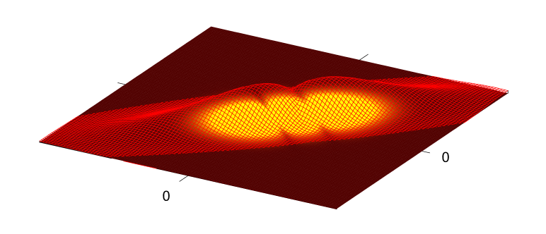
Figure 6: Intersecting heat maps are generated by converging trajectories, which project on the $xy$ plane their shared goal.

Once we have constructed heat maps for every trajectory, we define a similarity metric between two trajectories $T_{a}$ and $T_{b}$ as the volume under the combined heat surface $\Upsilon_{ab}$ obtained as the pointwise product of the two heat maps $H_{a}$ and $H_{b}$:

$$d^{k}_{\text{he}}(a,b)=\sum_{i=1}^{R}\sum_{j=1}^{C}\Upsilon_{ab}(i,j)=\sum_{i=1}^{R}\sum_{j=1}^{C}H_{a}(i,j)H_{b}(i,j)$$ (15)

The volume under $\Upsilon_{ab}$ reveals to what extent $T_{a}$ and $T_{b}$ have been close in space during the observation period, something that proxemics could already measure indeed. Nevertheless, heat maps relax the constraint by which only elements from the same frame can be compared, in practice this is accomplished through the thermal diffusion process. At the same time, heat maps also expose the history of their respective trajectories, allowing the metric to capture the temporal aspect of motion similarity. Proxemics, DTW and Granger causality would rate two pedestrians meeting and parting ways analogously, even if the former case is more likely to represent a group formation process. Recognizing motion trajectories also encode temporal information is a great advantage of heap maps based analysis.

6 Learning Framework

The linear parametrization of the affinity matrix $W_{\bf d}$ of Eq. (2) guarantees to reach a partition of the crowd which is consistent with the social groups properties. The parameters ${\bf w}=[{\boldsymbol{\alpha}},{\boldsymbol{\beta}}]$ govern both the importance of each feature alone and their similarity/dissimilarity optimal combinations, resulting in different clustering rules.

The choice of the best rule should account for all factors affecting the group formation process, such as environmental constraints or cultural influences. The complexity of explicitly evaluating these factors resides in the impossibility to directly observe them. Still, we can gain important insights by observing the grouping process. On these premises, we adopt a learning framework capable of choosing the most suitable clustering rule by finding a set of feature weights that implicitly embodies these non-observable aspects.

6.1 Supervised CC Through Structured Learning

Let us consider the input ${\bf x}_{i}=\{[{\bf 1}-{\bf d}^{i}(a,b);{\bf d}^{i}(a,b)]\}_{a,b}$ to be the set of pairwise features computed on all the possible pairs of trajectories $T_{a}$ and $T_{b}$ in the $i$-th temporal window and ${\bf y}_{i}$ the clustering solution, i.e. the set of all social groups appearing in the crowd $M_{i}$. Since ${\bf y}_{i}$ cannot be described by a single valued function, we adopt the Structural SVM [29] framework to model and learn predicting the solution. The goal is to learn a classification mapping $f:\mathcal{X}\rightarrow\mathcal{Y}$ between input space $\mathcal{X}$ and structured output space $\mathcal{Y}$ given a set of input-output pairs $\{({\bf x}_{1},{\bf y}_{1}),\dots,({\bf x}_{n},{\bf y}_{n})\}$. A discriminant score function $F:\mathcal{X}\times\mathcal{Y}\rightarrow\mathbb{R}$ is defined over the joint input-output space and $F({\bf x},{\bf y})$ can be interpreted as measuring the compatibility of ${\bf x}$ and ${\bf y}$. Now, the prediction function $f$ can be defined as

$$f({\bf x})~{}=~{}\arg\max_{{\bf y}\in\mathcal{Y}({\bf x})}F({\bf x},{\bf y})$$ (16)

where the maximizer over the label space $\mathcal{Y}({\bf x})$ is the predicted label, i.e. the solution of the inference problem. For simplicity we choose to restrict the space of $F$ to linear functions over some combined feature representation $\Psi({\bf x},{\bf y})$ subject to a ${\bf w}$ parametrization. This feature mapping cannot be defined out of the context of the problem, as it is the problem itself that specifies, given a particular input, the nature of the desired solution. Following the definition of correlation clustering in Eq. 1 and its parametrization introduced in Eq. 2, the compatibility of an input-output pair is directly described as

$$F({\bf x},{\bf y};{\bf w})={\bf w}^{T}\Psi({\bf x},{\bf y})={\bf w}^{T}\sum_{y\in{\bf y}}\sum_{a\neq b\in y}{\bf x}^{ab}.$$ (17)

The problem of learning in structured and interdependent output spaces can been formulated as a maximum-margin problem. We adopt the $n$-slack, margin-rescaling formulation:

$$\min_{{\bf w},{\bf\xi}} \frac{1}{2}\|{\bf w}\|^{2}+\frac{C}{n}\sum_{i=1}^{n}\xi_{i}$$ (18)

     s.t. $$\forall i:\xi_{i}\geq 0,$$

$$\forall i,\forall{\bf y}\in\mathcal{Y}({\bf x}_{i})\backslash{\bf y}_{i}:{\bf w}^{T}\delta\Psi_{i}({\bf y})\geq\Delta({\bf y},{\bf y}_{i})-\xi_{i},$$

where $\delta\Psi_{i}({\bf y})\overset{\text{def}}{=}\Psi({\bf x}_{i},{\bf y}_{i})-\Psi({\bf x}_{i},{\bf y})$, $\xi_{i}$ are the slack variables introduced in order to accommodate for margin violations, $\Delta({\bf y}_{i},{\bf y})$ is the loss function further defined in Sec. 6.3 and $C$ is the regularization trade-off. Intuitively, we want to maximize the margin and jointly guarantee that for a given input, every possible output result is considered worst than the correct one by at least a margin of $\Delta({\bf y}_{i},{\bf y})-\xi_{i}$, where $\Delta({\bf y}_{i},{\bf y})$ is bigger when the two predictions are known to be more different.

Remarkably, correlation clustering doesn’t need to know in advance how many groups are present in the scene. Moreover, a positive overall cluster score can group two elements even if their affinity measure is negative, implicitly modeling the transitive property of relationships in groups, as stated in Sec. 3.

6.2 Batch Sequential Optimization

The quadratic program (QP) (18) introduces a constraint for every possible wrong clustering of the $n$ examples, more precisely $\sum_{i=1}^{n}(|\mathcal{Y}({\bf x}_{i})|-1)$. Unfortunately, the number of ways to partition a set $M$ scales more than exponentially with the number of items according to the Bell sequence [41]

$$|\mathcal{Y}(M)|=\sum_{i=0}^{|M|}\frac{1}{i!}\sum_{j=0}^{i}(-1)^{i-j}{k\choose j}j^{|M|},$$ (19)

making the optimization intractable. As an example, for a crowd composed of 20 pedestrians the number of potential solutions would be about $5.8\cdot 10^{12}$. In order to deal with this high number of constraints many approximation schemes have been proposed, where cutting plane algorithms or subgradient methods are among the most commonly used. In particular, all the constraints of QP (18) can be replaced by $n$ piecewise-linear ones by defining the structured hinge-loss:

$$\widetilde{H}({\bf x}_{i})\overset{\text{def}}{=}\max_{{\bf y}\in\mathcal{Y}}\Delta({\bf y}_{i},{\bf y})-{\bf w}^{T}\delta\Psi_{i}({\bf y}).$$ (20)

The computation of the structured hinge-loss for each element $i$ of the training set, described in Sec. 6.4, amounts to finding the most “violating” output ${\bf y}$ for a given input ${\bf x}_{i}$ and its correct associated output ${\bf y}_{i}$. We only have $n$ constraints of the form $\xi_{i}\geq\tilde{H}({\bf x}_{i})$ and the non-smooth version of QP (18) reduces to

$$\min_{{\bf w}} \frac{1}{2}\|{\bf w}\|^{2}+\frac{C}{n}\sum_{i=1}^{n}\widetilde{H}({\bf x}_{i}).$$ (21)

By disposing of a maximization oracle, i.e. a solver for Eq. (20), and a computed solution ${\bf y}^{*}$, subgradient methods can easily be applied to QP (21), being $\partial_{\bf w}\widetilde{H}({\bf x}_{i})=-\delta\Psi_{i}({\bf y}^{*})$.

Algorithm 1 Block-Coordinate Frank-Wolfe Algorithm

1:  Let ${\bf w}^{(0)},{\bf w}_{i}^{(0)}:={\bf 0}$ and $l^{(0)},l_{i}^{(0)}:=0$

2:  for $\text{it}:=0$ to maxIterations  do

3:     Pick $i$ at random in $\{1,\dots,n\}$

4:     Solve ${\bf y}*:=\arg\max_{{\bf y}\in\mathcal{Y}}\Delta({\bf y}_{i},{\bf y})-{\bf w}^{T}\delta\Psi_{i}({\bf y})$

5:     Let ${\bf w}_{s}:=\frac{C}{n}\delta\Psi_{i}({\bf y}^{*})$ and $l_{s}:=\frac{C}{n}\Delta({\bf y}_{i},{\bf y}^{*})$

6:     Let $\gamma:=\frac{({\bf w}_{i}^{(\text{it})}-{\bf w}_{s})^{T}{\bf w}^{(\text{it})}+\frac{C}{n}(l_{s}-l_{i}^{(\text{it})})}{|{\bf w}_{i}^{(\text{it})}-{\bf w}_{s}\|^{2}}$ and clip to $[0,1]$

7:     Update ${\bf w}_{i}^{(\text{it}+1)}:=(1-\gamma){\bf w}_{i}^{(\text{it})}+\gamma{\bf w}_{s}$     and $l_{i}^{(\text{it}+1)}:=(1-\gamma)l_{i}^{(\text{it})}+\gamma l_{s}$

8:     Update ${\bf w}^{(\text{it}+1)}:={\bf w}^{(\text{it})}+{\bf w}_{i}^{(\text{it}+1)}-{\bf w}_{i}^{(\text{it})}$    and $l^{(\text{it}+1)}:=l^{(\text{it})}+l_{i}^{(\text{it}+1)}-l_{i}^{(\text{it})}$

9:  end for

To exploit the domain separability of the constraints and limit the number of oracle calls needed to converge to the optimal solution, we choose to adopt a Block-Coordinate version of the Frank-Wolfe algorithm (BCFW) [42], delineated in Alg. (1). The algorithm works by minimizing the objective function of Eq. (21) but restricted to a single random example at each iteration. By calling the max oracle upon the selected training sample (line 4) we obtain a new sub-optimal parameter set ${\bf w}_{s}$ by simple derivation (line 5). The best update is then found through a closed-form line search (line 6), greatly reducing convergence time compared to other subgradient methods.

In order to solve QP (21) effectively, it is important to choose an appropriate loss function as the learning ability of Structural SVM highly depends on it. In Sec. 6.3 we introduce and discuss different potential loss functions and their respective descriptive ability. Given the loss function, in Sec. 6.4 an efficient method to compute the maximization oracle (line 4 of Alg. 1) is described.

6.3 Loss Function and Scoring Procedure

One common choice of loss function for clustering is the pairwise loss $\Delta_{PW}({\bf y}_{i},{\bf y})$, which is a generalization of the Rand coefficient [43], and is defined as the ratio between the number of pairs on which ${\bf y}_{i}$ and ${\bf y}$ disagree on their cluster membership and the number of all possible pairs of elements in the set. Due to the quadratic number of connections that exist among crowd members, this measure tends to be imprecise when dealing with large crowds: as the crowdness increases, the number of positive links connecting group members becomes negligible with respect to the total number of links. As a consequence, erroneous solutions won’t be strongly penalized.
The MITRE loss [44], $\Delta_{M}({\bf y}_{i},{\bf y})$, founded on the understanding that connected components are sufficient to describe groups, partially mitigates this problem by representing groups as spanning trees, instead of complete graphs, inducing a linear amount of both positive and negative links among members (and not quadratic as in the pairwise case). For any crowd partitioning, a spanning forest is an equivalence class as many trees that describe the same group configuration may exist. The final score is obtained by accounting for the number of links that needs to be removed or added to recover a spanning forest of the correct solution. Nonetheless, problems arise when working on relations and not directly on members, as singletons have no connections at all but should still be considered positively when correctly classified.

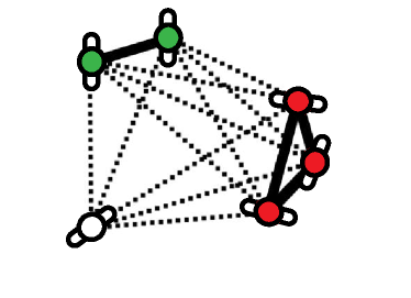
(a) ${\bf y}_{i}$ PAIRWISE links

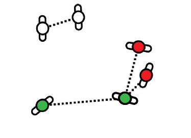
(b) ${\bf y},\Delta_{PW}({\bf y}_{i},{\bf y})=0.27$

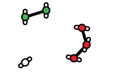
(c) ${\bf y}_{i}$ MITRE links

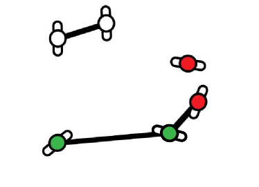
(d) ${\bf y},\Delta_{M}({\bf y}_{i},{\bf y})=0.6$

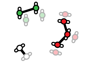
(e) ${\bf y}_{i}$ $G$-MITRE links

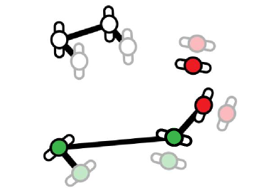
(f) ${\bf y},\Delta_{GM}({\bf y}_{i},{\bf y})=0.75$

Figure 7: Differences in the way losses account for errors. Singletons are white. Figures (a, c, e) depict solution ${\bf y_{i}}$ and the links considered by the respective losses, while (b, d, f) color pedestrians according to solution ${\bf y}$ and show the links on which the two solutions ${\bf y}_{i}$ and ${\bf y}$ disagree.

For this motivation, we propose a loss function, GROUP-MITRE loss ($G$-MITRE) $\Delta_{GM}({\bf y}_{i},{\bf y})$, that overcomes this limitation by adding, for each pedestrian described by the trajectory $T_{i}$, a fake counterpart $\alpha_{T_{i}}$ to which only singletons are connected. Through this shrewdness we can now take into consideration singletons as well when computing the discrepancy between two solutions. The particular design choice to link to the fake counterparts only singleton members generates two discrepancies when committing errors involving singletons and is thus a further effort in generating more plausible hierarchical groups in the solution, as depicted in Fig. 7. More formally, consider two clustering solutions ${\bf y}_{i}$, ${\bf y}$ and a representative of their respective spanning forests $Q$ and $R$. The connected components of $Q$ and $R$ are identified respectively by the set of trees $Q_{1},Q_{2},\dots$ and $R_{1},R_{2},\dots$. Note that if the number of elements in $Q_{j}$ is $|Q_{j}|$, then only $c(Q_{j})\stackrel{{\scriptstyle\text{\tiny def}}}{{=}}|Q_{j}|-1$ links are needed in order to create a spanning tree. Let us define $\pi_{\scriptscriptstyle R}(Q_{j})$ as the partition of a tree $Q_{j}$ with respect to the forest $R$, that is the set of subtrees obtained by considering only the membership relations in $Q_{j}$ also found in $R$. Besides, if $R$ partitions $Q_{j}$ in $|\pi_{\scriptscriptstyle R}(Q_{j})|$ subtrees then $v(Q_{j})\stackrel{{\scriptstyle\text{\tiny def}}}{{=}}|\pi_{\scriptscriptstyle R}(Q_{j})|-1$ links are sufficient to restore the original tree. It follows that the recall error for $Q_{j}$ can be computed as the number of missing links divided by the minimum number of links needed to create that spanning tree. Accounting for all trees $Q_{j}$ the global recall measure of $Q$ is:

$$\mathcal{R}_{Q}=1-\frac{\sum_{j}v(Q_{j})}{\sum_{j}c(Q_{j})}=\frac{\sum_{j}|Q_{j}|-|\pi_{\scriptscriptstyle R}(Q_{j})|}{\sum_{j}|Q_{j}|-1}$$ (22)

The precision of $Q$ (recall of $R$) can be computed by exchanging $Q$ and $R$. Given the definition of precision, recall and employing the standard $F$-score $F_{1}$, the loss is defined as

$$\Delta_{GM}=1-F_{1}.$$ (23)

The complete algorithm for the computation of the $G$-MITRE loss is reported in Alg. 2. We employ disjoint-set arrays due to the efficiency of checking whether two pedestrians belong to the same group. Recall that UNION and FIND are the standard functions defined over the disjoint-set arrays and denote the operations to merge two clusters and to find an element membership respectively. In the pseudo-code we use the notation ${\bf y}_{i}/{\bf y}$ to indicate that the algorithm first work on the solution ${\bf y}_{i}$ and then analogously on ${\bf y}$.

Algorithm 2 $G$-MITRE loss $\Delta_{GM}({\bf y}_{i},{\bf y})$ computation

0:  ${\bf y}_{i}$ and ${\bf y}$ as disjoint-set data structures

1:  $\varphi(x)$ are the unique roots of connected components $x$

2:  $\Gamma(x)$ is the size of the connected component with root $x$

3:  for all $T\in{\bf y}_{i}/{\bf y}$ do

4:     ${\bf y}_{i}/{\bf y}={\bf y}_{i}/{\bf y}\cup\alpha_{T}$

5:     if $\Gamma(\text{\footnotesize FIND}({\bf y}_{i}/{\bf y}(T))=1$ then

6:        $\text{\footnotesize UNION}({\bf y}_{i}/{\bf y}(T),{\bf y}_{i}/{\bf y}(\alpha_{T}))$

7:     end if

8:  end for

9:  for all $q\in\varphi({\bf y}_{i}/{\bf y})$ do

10:     $v_{{\bf y}_{i}/{\bf y}}~{}{+=}~{}|\varphi(\bigcup_{\text{\scriptsize FIND}({\bf y}_{i}/{\bf y}(T))=q}{\bf y}/{\bf y}_{i}(T))|-1$

11:     $c_{{\bf y}_{i}/{\bf y}}~{}{+=}~{}\Gamma(q)-1$

12:  end for

13:  $\mathcal{R}_{{\bf y}_{i}/{\bf y}}=1-v_{{\bf y}_{i}/{\bf y}}/c_{{\bf y}_{i}/{\bf y}}$

14:  $\Delta({\bf y}_{i},{\bf y})=1-2\mathcal{R}_{{\bf y}_{i}}\mathcal{R}_{{\bf y}}/(\mathcal{R}_{{\bf y}_{i}}+\mathcal{R}_{{\bf y}})$

6.4 Approximate Oracle

Despite the simplicity of the algorithm, the intrinsic complexity of the optimization is hidden in the search for the most violating solution ${\bf y}^{*}$ for the $i$-th example (line 4 of Alg. (1)): finding the most violated constraint requires to solve the loss augmented decoding subproblem. Note that the original prediction problem of Eq. (16) is NP-hard and the insertion of a non-linear loss in the computation of the maximum is not likely to help. Nevertheless, thanks to its iterative nature, the inference scheme introduced in Sec. 4 can be adapted to approximate the oracle as well. Starting from the trivial solution having each pedestrian of the $i$-th example in its own cluster, the algorithm repeatedly merges the two clusters which reflect in the highest increment in the structured hinge-loss $\tilde{H}({\bf x}_{i})$ of Eq. (20), until a local maxima is found.

Of course by following a greedy procedure, there is no guarantee to select the most violated constraint. Interestingly enough, Lacoste-Julien et al. [42] show that all convergence results known for exact maximizer of the loss augmented problem also hold for approximate maximizers by allowing the algorithm to iterate longer toward convergence. For further details, please refer to their original work.

TABLE II: Comparative results on publicly available dataset using the $G$-MITRE loss of Sec. 6.3 and the positive pairwise loss $\Delta_{PW}^{+}$ of [26].

		our method		baseline		[2]		[24]		[26]		[21]
		$\mathcal{P}$	$\mathcal{R}$	$\mathcal{P}$	$\mathcal{R}$	$\mathcal{P}$	$\mathcal{R}$	$\mathcal{P}$	$\mathcal{R}$	$\mathcal{P}$	$\mathcal{R}$	$\mathcal{P}$	$\mathcal{R}$
BIWI	$\Delta_{GM}$	97.3 $\pm$ 0.7	97.7 $\pm$ 1.5	71.0 $\pm$ 8.1	69.6 $\pm$ 7.4	89.2	90.9	84.0	51.2			67.3	64.1
hotel	$\Delta_{PW}^{+}$	89.1 $\pm$ 1.2	91.9 $\pm$ 1.5	47.6 $\pm$ 9.2	88.6 $\pm$ 8.6	88.9	89.3	83.7	93.9	81.0	91.0	51.5	90.4
BIWI	$\Delta_{GM}$	91.8 $\pm$ 1.2	94.2 $\pm$ 0.9	72.4 $\pm$ 4.4	65.2 $\pm$ 3.4	87.0	84.2	60.6	76.4			69.3	68.2
eth	$\Delta_{PW}^{+}$	91.1 $\pm$ 0.4	83.4 $\pm$ 0.6	39.1 $\pm$ 8.4	91.2 $\pm$ 1.7	80.7	80.7	72.9	78.0	79.0	82.0	44.5	87.0
CBE	$\Delta_{GM}$	81.7 $\pm$ 0.2	82.5 $\pm$ 0.2	59.9 $\pm$ 2.9	53.5 $\pm$ 6.8	77.2	73.6	56.7	76.0			40.4	48.6
student003	$\Delta_{PW}^{+}$	82.3 $\pm$ 0.3	74.1 $\pm$ 0.2	24.0 $\pm$ 9.7	49.3 $\pm$ 12.9	72.2	65.1	63.9	72.6	70.0	74.0	10.6	76.0

7 Experimental Results

We designed several experiments to evaluate the algorithm behavior on well-assessed benchmarks and its connections to the nature of the problem. All the experiments were carried out on ground truth trajectory data, except for Sec. 7.4 where the method is evaluated on tracklets extracted by a modern detector/tracker system. We also propose new video sequences to stress the algorithm over a variety of challenges in real world scenarios. Since the method works on ground plane (metric) data, we also provide homography information for all the employed sequences.

Datasets

We selected two publicly available datasets, namely the BIWI Walking Pedestrians dataset [45] and the Crowds-By-Examples (CBE) dataset [46]. The former dataset records two low crowded scenes, outside a university and at a bus stop (eth and hotel in Tab. III). The CBE dataset records a medium density crowd outside another university (student003, briefly stu003) providing some challenges: the density of the pedestrians is significantly high and the presence of multiple entry and exit points. While BIWI and CBE are standard datasets in crowd analysis, we also use the more recent Vittorio Emanuele II Gallery (VEIIG) dataset [47], from which we extracted a five minutes subsequence, gal1, particularly interesting due to the fast and continuous change in crowd density. We also propose a new dataset to cope with the increasing variety of application in dense-crowd management, MPT-$20$x$100$, composed of 20 sequences of 100 frames where we manually annotated trajectories and social groups. The dataset comprises different videos [48] all characterized by a high number of pedestrians with an heterogeneous set of scene conditions, ranging from density, scale, viewpoint and type of interactions, like walking in a mall, crossing the street or participating at public events.
In Tab. III we report some measures useful to characterize the spatial complexity of the datasets:

• $d_{\text{in}}$ is the group compactness, computed as the mean distance between members of the same groups;

• $d_{\text{out}}$ is the group isolation or the mean distance between each member and its closest unrelated pedestrian;

• the ratio $d_{\text{i/o}}\stackrel{{\scriptstyle\text{\tiny def}}}{{=}}d_{\text{in}}/d_{\text{out}}$ measures crowd collectiveness: small values mean compact groups in a sparse crowd.

TABLE III: Datasets: number of pedestrians (#p), groups (#g) and density metrics.

	#p	#g	$d_{\text{in}}~{}(m)$	$d_{\text{out}}~{}(m)$	$d_{\text{i/o}}$
student003	406	108	0.41	0.70	0.59
eth	117	18	0.99	2.79	0.35
hotel	107	11	0.75	2.00	0.38
gal1	630	207	0.77	1.66	0.46
MPT-20x100	82	10	0.63	1.45	0.48

Evaluation Scheme

There is no consensus on which metrics should be used to evaluate groups correctness: we propose to use the $G$-MITRE precision $\mathcal{P}$ and recall $\mathcal{R}$ since it accounts for the correct classification of singletons as well. This is an important gain as in crowded scenes the number of people walking alone is rarely negligible. Each measure is reported in terms of mean and standard deviation over 5 runs to account for the stochastic nature of the training of our algorithm. Where not differently specified, we used a 100s for training and a 10s sliding window with no overlap for features computation. The regularization parameter $C$ of QP. (18) is fixed to 10.

For the heat-map based feature of Sec. 5.3, we run a grid search on the parameters. For all the experiments, the length of the cells edge is fixed to 30cm, $k_{s}=10^{-5}$ and $k_{r}=0.5$.

7.1 Baseline and Benchmark Comparisons

We compare our method with three recent state of the art group detection algorithms, namely [2, 24, 26, 21], selected on the basis of their reported performances on public datasets and availability of code. In addition, we devised a simple baseline version of our solution that performs the group partitioning with no use of the learning framework. The weights are randomly chosen to be the same for all the features, so that the randomness resides in the similarity/dissimilarity ratio.

TABLE IV: Evaluation of our proposal when trained with different loss functions.

	Pairwise $\Delta_{PW}$		MITRE $\Delta_{M}$
	$\mathcal{P}$	$\mathcal{R}$	$\mathcal{P}$	$\mathcal{R}$
hotel	90.1 $\pm$ 2.0	84.1 $\pm$ 3.2	89.2 $\pm$ 3.0	93.2 $\pm$ 1.9
eth	88.7 $\pm$ 1.8	87.3 $\pm$ 2.6	91.9 $\pm$ 0.8	92.9 $\pm$ 1.0
stu003	68.9 $\pm$ 1.4	69.9 $\pm$ 1.5	80.1 $\pm$ 2.4	80.9 $\pm$ 2.3

7.1.1 Quantitative Results

Quantitative results are given in Tab. II. To highlight our algorithm superiority, results are presented both in terms of $G$-MITRE and a pairwise loss accounting only for positive (intra-group) relations but neglecting singletons, $\Delta_{PW}^{+}$ [26]. The latter loss is not directly optimized by our algorithm, still our method outperforms the competitors in all the tested sequences. This can be explained through the ability of our algorithm to adapt the concept of groups to always different scenario by varying the feature importance and the use of sociologically inspired similarity functions. The slightly lower performances on the stu003 sequence are due to the high complexity of the scene: the high value of the $d_{\text{i/o}}$ ratio in Tab. III suggests the presence of loose groups in a dense crowd and, as such, challenging to be detected.

7.1.2 Evaluation of Different Loss Functions

As structured learning relies upon a definition of what’s wrong to learn how to classify well, the choice of the loss function can greatly affect the final performances. By fixing the $G$-MITRE measure as a proper scoring scheme, we quantitatively test the influence of the choice of the loss on the eth, hotel and stu003 datasets (Tab. IV). As it could be expected by its definition, the improvement due to the use of the $G$-MITRE loss (reported in Tab. II) is greater in the eth and hotel sequences where the ratio between the number of singletons and the people walking in groups is higher and as such learning to classify them as well becomes crucial. More interestingly, we observe how the pairwise loss obtains outstanding performances when the number of pedestrians is limited, but becomes ineffective when it starts to grow, as in stu003.

7.2 Features Weight Learning on MPT-${\bf 20}$x${\bf 100}$

CBE and BIWI datasets expose some interesting challenges of the problem but, with the only exception of stu003 sequence, they have a limited number of pedestrians in scene and a low crowd density. Moreover, the scenarios are similar and the variety of interactions underlying the group formation is limited. The proposed MPT-$20$x$100$ datasets, on the other hand, presents different degrees of complexity.

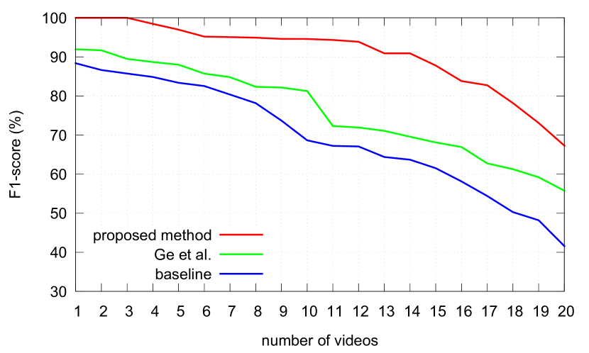
Figure 8: Comparison against baseline and [2] on MPT-$20$x$100$.

First, we evaluate the general performance of the algorithm and compare with both our baseline and the proposal in [2] where, for the latter method, we manually tuned the thresholds to achieve best results. These methods are clustering based, partially consistent with the social group axioms but no learning is employed. Results are shown in Fig. 8 as a survival curve plot which reveals on how many sequences the algorithms where at least able to reach the specific lower-bound performance and per-video scores are in Fig. 9. Interestingly, the difference between our method and [2] increases here with respect to the previous datasets on an average of 10%, suggesting that sequences can be really different in the concept of groups they embed and thus learning is mandatory to adapt to this new representations of social groups and keep performances stable.

7.2.1 The Need for Learning from Examples

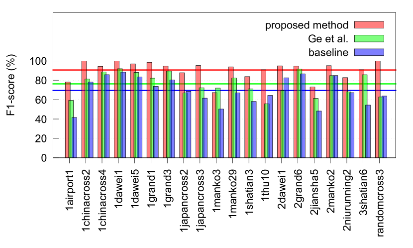
Figure 9: Results on MPT-$20$x$100$ highlight the complexity of each scene.

The confusion-like matrix, depicted in Fig. 10, presents the F-1 scores obtained by training the algorithm on one sequence of MPT-$20$x$100$ (row labels) and testing it on all the other sequences (column labels). By reading the matrix, and averaging each row over all the columns, it is possible to grasp how good a particular sequence was for training. At the same time, by observing the average of the columns over all the rows, we can get intuition about how much each sequence was effectively predicted by all the others.
We are interested in understanding whether a specific notion of group is shared across sequences and how it is influenced by both scene elements (e.g. crowd density) and unobserved aspects (e.g. intentions and social hierarchies).

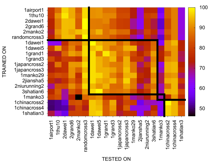
Figure 10: F-1 scores obtained by all combinations of train/test pair sequences in MPT-$20$x$100$. Results were clustered (diagonal blocks C1-C4 from left to right) to highlight similar notion of group among sequences.

With the purpose of capturing these invariants, we search the connected component of the matrix using the F-1 score as the affinity value among elements. Clustering is performed through an asymmetric version of spectral clustering [49] based on the Random Walk Laplacian defined as

$$L=AD^{-1},$$ (24)

where $A$ is the affinity matrix defined as in Fig. 10 and $D$ is the usual degree matrix. Following the eigen-gap heuristic we found $4$ distinct clusters in the MPT-$20$x$100$ dataset, highlighted with black lines in Fig. 10; for every cluster we computed the $d_{\text{in}}$, $d_{\text{out}}$ and $d_{\text{i/o}}$ spatial measures, displayed in Tab. V, to verify if clusters with a similar notion of group also share a common configuration of distances among pedestrians and possibly if the performance are connected to crowd density.

TABLE V: Spatial depiction, training efficacy and groups predictability of the clusters of sequences of Fig. 10.

cluster	$d_{\text{in}}$ (m)	$d_{\text{out}}$ (m)	$d_{\text{i/o}}$	$\text{F}_{1}$ train	$\text{F}_{1}$ test
C1	0.58	1.03	0.54	0.82	0.82
C2	0.59	1.28	0.47	0.85	0.84
C3	0.59	0.99	0.59	0.77	0.64
C4	0.89	3.00	0.34	0.75	0.84

Tab. V also reports a measure of training efficacy (F₁ train), computed as the mean accuracy obtained on the whole dataset when only sequences in that specifi cluster were used for training and, analogously, a group predictability score (F₁ test) or the mean accuracy obtained on the sequences of that cluster when all the sequences were used for training. They indicate how much a cluster is useful during training and easy it is to predict groups inside its sequences.

A first observation that can be made is about the cluster C4, which presents the highest F₁ test and the lowest F₁ train. We found it was easy to predict groups in these videos but they were poorly informative as training examples, a result justified by its small $d_{\text{i/o}}$. Nonetheless, clusters 1 and 3 exhibits very similar $d_{\text{i/o}}$ ratio but perform very differently in terms both of training efficacy and testing score, suggesting a trivial heuristic based on spatial information only is insufficient to visually discern groups. Implicit aspects like motion constraints or cultural and social context also affect the group process formation, defending our hypothesis that learning is needed to adapt the concept of group to the current data.

7.2.2 Do we Capture the Essence of Being a Group?

As previously stated, MPT-$20$x$100$ comprises very different scenarios and situations and can provide important insights on which are the most important elements that reveal groups. To this end, recall the definition of feature vector ${\bf w}=[\boldsymbol{\alpha},\boldsymbol{\beta}]=[w_{1},w_{2},\dots,w_{8}]$ from Eq. (2) of Sec. 4 is such that the affinity between two trajectories $T_{a}$ and $T_{b}$ can be written as:

$$W^{ab}_{\bf d} ={\boldsymbol{\alpha}}^{T}({\bf 1}-{\bf d}(a,b))-{\boldsymbol{\beta}}^{T} {\bf d}(a,b)$$ (25)

$$=w_{1}+w_{2}+w_{3}+w_{4}- [(w_{5}+w_{1})d_{ph}+\dots$$

$$~{}(w_{6}+w_{2})d_{sh}+\dots$$

$$~{}(w_{7}+w_{3})d_{ca}+\dots$$

$$\underbrace{\hskip 85.35826pt\vphantom{]}}_{\text{constant term}}{} \underbrace{(w_{8}+w_{4})d_{he}}_{\text{$(a,b)$-dependent term}}]$$

The contribution of each feature to the score, transformed from a distance to an affinity measure by the constant term of Eq. (25), is encoded in the absolute value of the coefficient of the features themselves.

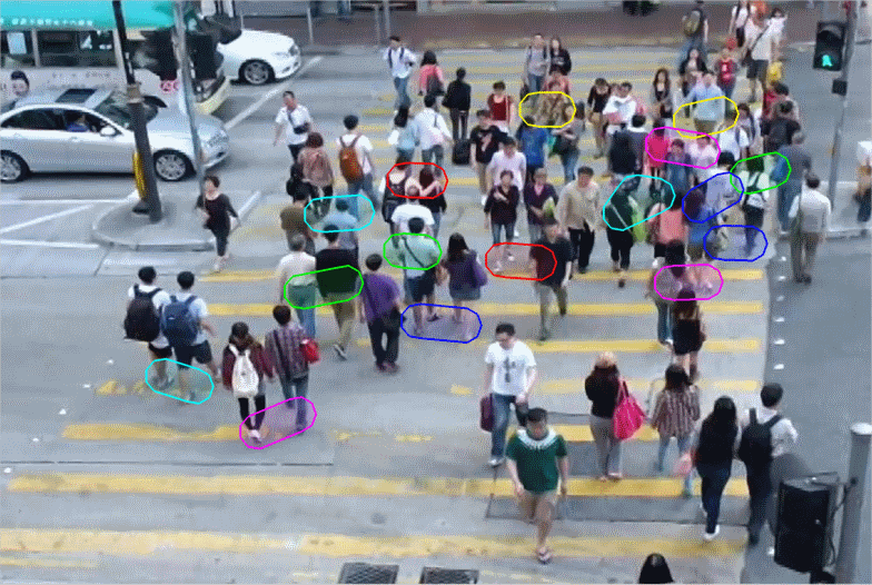
(b) 1manko3

(c) 2jiansha5

(d) randomcross3

(e) 3shatian6

(f) seq1

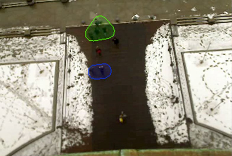
(g) eth

(h) hotel

Figure 15: Examples of groups detected through our method: sequences from (a) to (e) are from the MPT-$20$x$100$, while (f) is part of GVEII and finally, (g) and (h) belong to the BIWI dataset. Groups are identified regardless of the scene context and errors are visually acceptable, as in (d).

As shown in Fig. 11, the proxemic inspired feature $d_{ph}$ dominates all the others while the importance of the remaining features vary greatly from sequence to sequence. The two sequences 1manko3 (Fig. 15) and 1dawei1 (Fig. 1), for example, present very similar contribution from $d_{\text{hm}}$ and $d_{\text{sh}}$, while the importance assigned to $d_{\text{ph}}$ in 1dawei1 is shifted to $d_{\text{ca}}$ in 1manko3. The former sequence present a particularly sparse crowd, making distance among elements a strong peculiarity of groups, but when the space among pedestrian is reduced both intra and inter-groups distances (and consequently $d_{\text{ph}}$) become less significant. Conversely, the causality feature $d_{ca}$ becomes more important when the density increases as pedestrians tend to follow each others to avoid getting separated from the rest of the group.

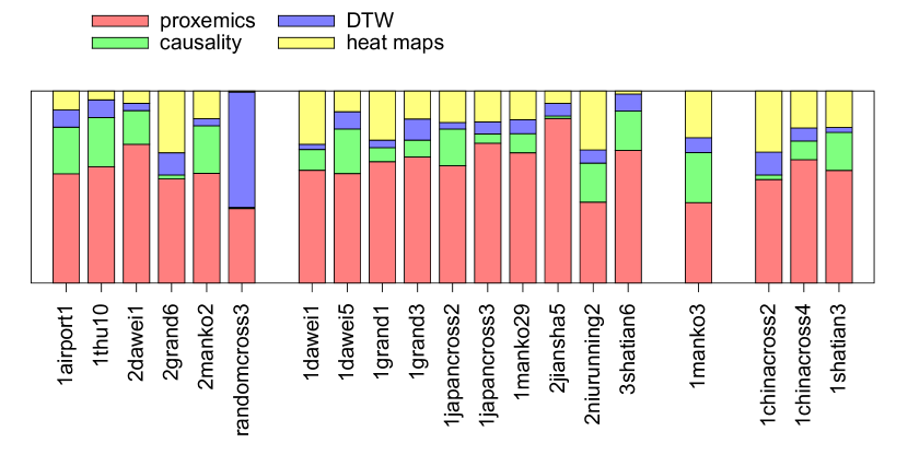
Figure 11: Features normalized coefficients of Eq. (25).

Heat maps importance gain emphasis from comparing 1manko3 and 3shatian6 (Fig. 15), as they are very helpful in decoupling trajectories that stand very close in space but for a very limited amount of time. In particular, in 1manko3, people crossing from opposite sides of the road tend to be very close when meeting in the middle, even if they are not in the same group.

TABLE VI: Performance of detector [50], tracker [51] and group detection algorithms (in terms of G-MITRE) in a fully automatic pipeline.

	Detector		Tracker				our proposal		[2]		[24]		[21]
	$\mathcal{P}$	$\mathcal{R}$	MOT(A/P)	MT	IDS	FRG	$\mathcal{P}$	$\mathcal{R}$	$\mathcal{P}$	$\mathcal{R}$	$\mathcal{P}$	$\mathcal{R}$	$\mathcal{P}$	$\mathcal{R}$
hotel	43.1	52.4	66.9 / 0.88	18.8	120	34	77.9	76.9	75.7	78.0	46.3	38.6	60.2	57.5
eth	68.2	53.7	92.3 / 0.08	75.0	0	68	81.1	79.7	78.4	79.3	58.3	70.6	57.3	61.2
student	56.7	36.8	43.3 / 1.22	06.0	342	876	75.0	71.3	63.2	56.4	40.2	52.4	35.1	40.2

7.3 Evaluating the Influence of Density Changes

In this test setting we evaluate if the feature weights learned by the Structural SVM of Sec. 6 are sufficiently general to deal with crowds at different densities and, at the same time, understand whether an online version of Alg. 1 would bring any accuracy improvement. To this end we introduce a new video sequence, gal1 from GVEII, containing an average number of $70$ pedestrians simultaneously present in the scene. The distribution of pedestrians is not uniform though, and increases over time, as well as for their density, represented by the $d_{\text{i/o}}$ ratio (Fig. 12).

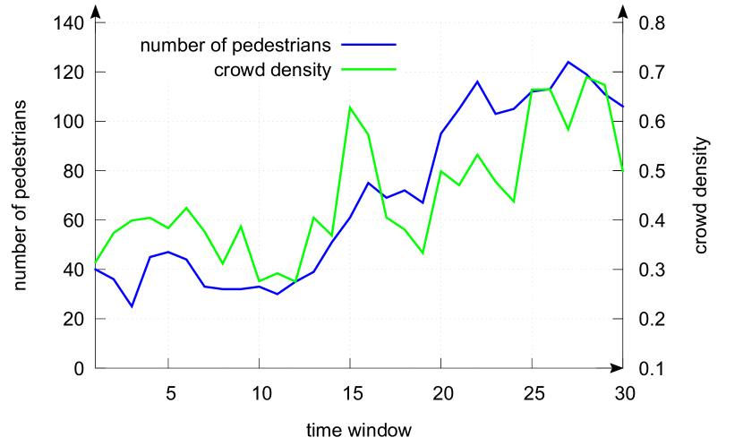
Figure 12: Pedestrians number and $d_{\text{i/o}}$ ratio temporal evolution in the gal1 sequence of GVEII.

In order to underline the importance of capturing changes in density, we compare the batch version of the training algorithm Alg. 1 with a sequential and a fully online version (Fig. 13). In the former case, examples are fed to the supervised training procedure in temporal order one at a time, while for the latter case, the weights have been initialize to the ones learned batch and the algorithm at each step learns from the previous prediction, thus without supervision.
The plot in Fig. 13 shows the performance of the batch training version tends to decrease as the crowd density increases. While the sequential version of the algorithm performs better, it is slow to respond to sudden density changes like in time windows $15$. Indeed, a non-smooth density variation affects negatively the training process, leading to a performance drop further recovered in the subsequent temporal windows. Eventually, this behavior is partially mitigated in the fully online version. The higher performances are motivated by the implicit regularization: using the prediction as training input discourages the learner to drastically modify the weights vector and mimic the smooth variation in crowd density slightly adjusting in time.

7.4 Performances on Real Detector and Tracker

Our algorithms assumes the availability of correct trajectories to detect groups, but what happens in a fully automatic video surveillance pipeline where a people detector and tracker are employed? We carried out experiments by extracting pedestrian positions through a state of the art detector [50] and obtaining trajectories by means of a continuous energy minimization method [51]. We compare with Ge et al. [2], Yamaguchi et al. [24] and Shao et al. [21] over the same input data, results are shown in Tab. VI. Our proposal outperforms the competitors even in the case of noisy trajectories.

Tracking performances evidence a high number of tracks fragments, namely FRG, that are mainly due to the localization error introduced by the automatic people detector on non-trivial crowded scenes. FRGs are proportional to the number of small new tracks created by the system instead of correctly associating previously tracked objects, with the consequence of splitting ideal tracks into temporally disjoint segments.
A high FRG number affects the group detection performance as the $d_{ph}$ and $d_{ca}$ features are computed when the trajectories are simultaneously present in the scene and thus merging temporal disjoint fragments is strongly discouraged by the correlation clustering algorithm. Intuitively, by reducing the size of the window we are able to minimize the number of split trajectories at each example and recover most of the original performances, as shown in Fig. 14(c). The improvement is basically achieved through the joint adoption of socially founded features and structural learning that weights the features according to the observed noisy trajectories. The experiment allow us to conclude that even in the case of a real application and imprecise input data the strengths of the proposed algorithm are maintained because are strongly related to the social rules that govern the group formation process, these rules are not data dependent and hold despite the applied feature extraction techniques.

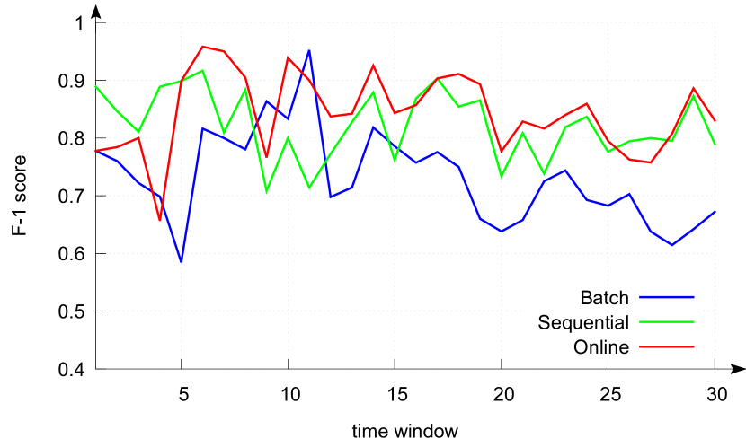
Figure 13: F-1 score comparison between differently trained version of the our method on gal1 of GVEII.

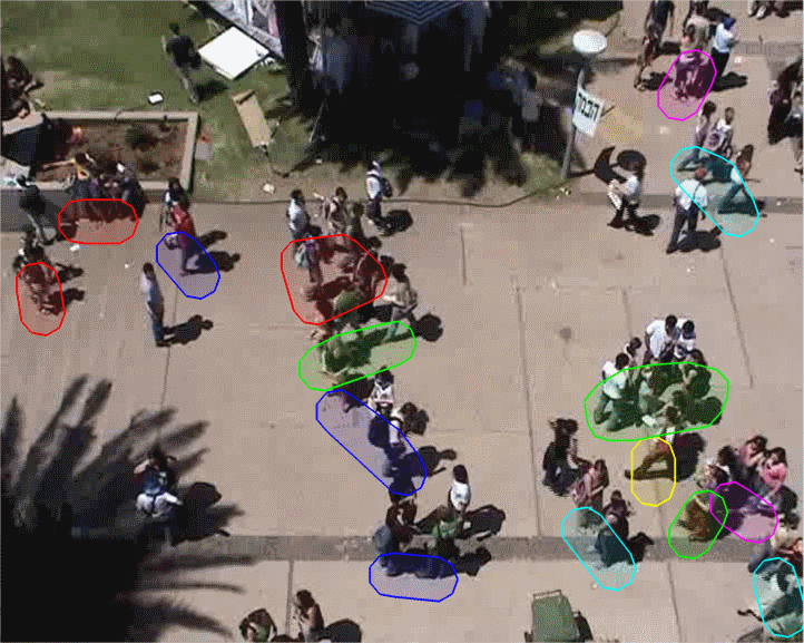
(a)

(b)

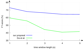
(c)

Figure 14: Group detection results on student003 are displayed when corrected tracks are used (a) and when input with people detector and tracker automatic responses (b). Regardless of the input noise, most of the groups can still be identified. This is due to the robustness of the features employed during learning and to the decrease in length of the time window (c) which prevents fragmented tracks to be split in different groups.

(a) 1airport1

8 Conclusion

In this work, we pointed out the need to approach the task of detecting social groups in crowds from a learning perspective. Many existing methods rely on specifically tuned parameters that limit their applicability in real world scenarios. Our intuition is that there are crowds that preserve the same concept of social group, but in many cases this concept cannot be distilled from spatial consideration only. We thus defined a set of social-inspired and strongly motivated features able to capture and characterize different groups peculiarities. To learn a socially meaningful clustering rule to group pedestrians, we relied on the Structural SVM framework and designed a peculiar loss function able to account for singletons as well as for group errors. Even though the algorithm was originally designed to work with exact trajectories, we replicated the experiments on noisy tracklets extracted by a detector/tracker obtaining state-of-the-art results. Moreover, we proposed an online training version of the method, able to achieve superior generalization performances on crowds with variable density.

We did note, however, that as we consider wider portions of the scene, the chance that many different densities groups coexist in different locations increases, leading to the necessity to learn more than one clustering rule per scene. To resolve this problem we plan, as future work, to learn a set of different distance measures and use latent variables to choose the most appropriate given a particular zone. Code and datasets are made publicly available in order to reproduce this paper results and allow the community to improve the proposed method.

Francesco Solera obtained a master degree in computer engineering from the University of Modena and Reggio Emilia in 2013. He is now a PhD candidate within the ImageLab group in Modena, researching on applied machine learning and social computer vision.

Simone Calderara received a computer engineering master degree in 2004 and a PhD degree in 2009 from the University of Modena and Reggio Emilia, where he is now an assistant professor within the Imagelab group. His current research interests include computer vision and machine learning applied to human behavior analysis, visual tracking in crowded scenarios and time series analysis for forensic applications.

Rita Cucchiara received her master degree in electronic engineering and the PhD degree in computer engineering from the University of Bologna, Italy, in 1989 and 1992 respectively. Since 2005, she is a full professor at University of Modena and Reggio Emilia, Italy, where she heads the ImageLab group and the SOFTECH-ICT research center. Her research focuses on pattern recognition, computer vision and multimedia.

References

- [1] L. Manenti, S. Manzoni, G. Vizzari, K. Ohtsuka, and K. Shimura, “An agent-based proxemic model for pedestrian and group dynamics: motivations and first experiments,” in Multi-Agent-Based Simulation XII, ser. LNCS. Springer Berlin Heidelberg, 2012, pp. 74–89.
- [2] W. Ge, R. Collins, and R. Ruback, “Vision-based analysis of small groups in pedestrian crowds,” IEEE Trans. Pattern Analysis and Machine Intelligence, vol. 34, pp. 1003–1016, May 2012.
- [3] M. Moussaid, N. Perozo, S. Garnier, D. Helbing, and G. Theraulaz, “The walking behaviour of pedestrian social groups and its impact on crowd dynamics,” PLoS ONE, vol. 5, Apr. 2010.
- [4] B. E. Moore, S. Ali, R. Mehran, and M. Shah, “Visual crowd surveillance through a hydrodynamics lens,” Commununications of the ACM, vol. 54, pp. 64–73, Dec. 2011.
- [5] D. Helbing and P. Molnár, “Social force model for pedestrian dynamics,” Physical Review E, vol. 51, pp. 4282–4286, May 1995.
- [6] J. C. Turner, “Towards a cognitive redefinition of the social group,” Current Psychology of Cognition, vol. 1, pp. 93–118, jun 1981.
- [7] N. Bansal, A. Blum, and S. Chawla, “Correlation clustering,” Machine Learning, vol. 56, pp. 89–113, Jul. 2004.
- [8] T. Joachims, T. Finley, and C.-N. J. Yu, “Cutting-plane training of structural SVMs,” Machine Learning, vol. 77, pp. 27–59, Oct. 2009.
- [9] S. Pellegrini, A. Ess, and L. Van Gool, “Improving data association by joint modeling of pedestrian trajectories and groupings,” in Proc. Eur. Conf. Computer Vision (ECCV), 2010, pp. 452–465.
- [10] G. Bon, The Crowd: a Study of the Popular Mind. Kessinger Publishing, 1896.
- [11] A. G. Ingham, G. Levinger, J. Graves, and V. Peckham, “The ringelmann effect: Studies of group size and group performance,” Journal of Experimental Social Psychology, vol. 10, pp. 371–384, Jul. 1974.
- [12] R. Mehran, A. Oyama, and M. Shah, “Abnormal crowd behavior detection using social force model,” in Proc. IEEE Int’l Conf. Computer Vision and Pattern Recognition (CVPR), 2009, pp. 935–942.
- [13] M. Luber, J. Stork, G. Tipaldi, and K. Arras, “People tracking with human motion predictions from social forces,” in Proc. Int’l Conf. Robotics and Automation (ICRA), 2010, pp. 464–469.
- [14] S. Bandini, A. Gorrini, L. Manenti, and G. Vizzari, “Crowd and pedestrian dynamics: Empirical investigation and simulation,” in Proc. Measuring Behavior, Int’l Conf. Methods and Techniques in Behavioral Research, 2012, pp. 308–311.
- [15] S. D. Reicher, R. Spears, and T. Postmes, “A social identity model of deindividuation phenomena,” European Review of Social Psychology, vol. 6, pp. 161–198, Jan. 1995.
- [16] M. Rodriguez, I. Laptev, J. Sivic, and J.-Y. Audibert, “Density-aware person detection and tracking in crowds,” 2011, pp. 2423–2430.
- [17] F. Solera, S. Calderara, and R. Cucchiara, “Structured learning for detection of social groups in crowd,” in Proc. IEEE Int’l Conf. Advanced Video and Signal Based Surveillance (AVSS), 2013, pp. 7–12.
- [18] A. Kendon, Conducting Interaction: patterns of Behavior in Focused Encounters. Cambridge University Press, 1990.
- [19] M. Cristani, L. Bazzani, G. Paggetti, A. Fossati, D. Tosato, A. Del Bue, G. Menegaz, and V. Murino, “Social interaction discovery by statistical analysis of f-formations,” 2011, pp. 1–12.
- [20] M. Feldmann, D. Fränken, and W. Koch, “Tracking of extended objects and group targets using random matrices,” IEEE Trans. Signal Processing, vol. 59, pp. 1409–1420, Apr. 2011.
- [21] J. Shao, C. C. Loy, and X. Wang, “Scene-independent group profiling in crowd,” in Proc. IEEE Int’l Conf. Computer Vision and Pattern Recognition (CVPR), 2014.
- [22] S. K. Pang, J. Li, and S. Godsill, “Detection and tracking of coordinated groups,” IEEE Trans. Aerospace and Electronic Systems, vol. 47, pp. 472–502, Jan. 2011.
- [23] L. Bazzani, Cristani, and V. Murino, “Decentralized particle filter for joint individual-group tracking,” in Proc. IEEE Int’l Conf. Computer Vision and Pattern Recognition (CVPR), 2012, pp. 1886–1893.
- [24] K. Yamaguchi, A. Berg, L. Ortiz, and T. Berg, “Who are you with and where are you going?” in Proc. IEEE Int’l Conf. Computer Vision and Pattern Recognition (CVPR), 2011, pp. 1345–1352.
- [25] M. C. Chang, N. Krahnstoever, and W. Ge, “Probabilistic group-level motion analysis and scenario recognition,” 2011, pp. 747–754.
- [26] M. Zanotto, L. Bazzani, M. Cristani, and V. Murino, “Online bayesian non-parametrics for social group detection,” in Proc. British Machine Vision Conference (BMVC), 2012, pp. 111.1–111.12.
- [27] E. Canetti, Crowds and Power. Farrar, Straus and Giroux, 1984.
- [28] C. McPhail and R. T. Wohlstein, “Using film to analyze pedestrian behavior,” Sociological Methods & Research, vol. 10, no. 3, pp. 347–375, Feb. 1982.
- [29] I. Tsochantaridis, T. Joachims, T. Hofmann, and Y. Altun, “Large margin methods for structured and interdependent output variables,” Journal of Machine Learning Research, vol. 6, p. 1453–1484, Sep. 2005.
- [30] J. Kleinberg, “An impossibility theorem for clustering,” in Advances in Neural Information Processing Systems, 2002, pp. 446–453.
- [31] E. Hall, The hidden dimension. Doubleday, 1966.
- [32] S. Calderara and R. Cucchiara, “Understanding dyadic interactions applying proxemic theory on videosurveillance trajectories,” in Proc. IEEE Int’l Conf. Computer Vision and Pattern Recognition Workshops (CVPRW), 2012, pp. 20–27.
- [33] M. Cristani, G. Paggetti, A. Vinciarelli, L. Bazzani, G. Menegaz, and V. Murino, “Towards computational proxemics: Inferring social relations from interpersonal distances,” in Proc. IEEE Int’l Conf. Social Computing, 2011, pp. 290–297.
- [34] S. Haslam, Psychology in Organizations. SAGE Publications, 2004.
- [35] J. Oldmeadow, M. J. Platow, and M. Foddy, “Task-groups as self-categories: a social identity perspective on status generalization,” Current Research in Social Psychology, vol. 10, pp. 268–283, Aug. 2005.
- [36] C. W. J. Granger, “Investigating causal relations by econometric models and cross-spectral methods,” Econometrica, vol. 37, pp. 424–438, Aug. 1969.
- [37] I. D. Couzin, J. Krause, N. R. Franks, and S. A. Levin, “Effective leadership and decision-making in animal groups on the move,” Nature, vol. 433, pp. 513–516, Feb. 2005.
- [38] M. Hazewinkel, Encyclopaedia of Mathematics. Springer, 1989, vol. 4.
- [39] D. Berndt and J. Clifford, “Using dynamic time warping to find patterns in time series,” in Proc. ACM Int’l Conf. Knowledge Discovery and Data Mining Workshops (KDDW), 1994, pp. 359–370.
- [40] W. Lin, H. Chu, J. Wu, B. Sheng, and Z. Chen, “A heat-map-based algorithm for recognizing group activities in videos,” IEEE Trans. Circuits and Systems for Video Technology, vol. 23, pp. 1980–1992, Nov. 2013.
- [41] G.-C. Rota, “The number of partitions of a set,” The American Mathematical Monthly, vol. 71, pp. 498–504, May 1964.
- [42] S. Lacoste-Julien, M. Jaggi, M. Schmidt, and P. Pletscher, “Block-coordinate frank-wolfe optimization for structural SVMs,” in Proc. Int’l Conf. Machine Learning (ICML), 2013, pp. 53–61.
- [43] W. M. Rand, “Objective criteria for the evaluation of clustering methods,” Journal of the American Statistical Association, vol. 66, pp. 846–850, Dec. 1971.
- [44] M. Vilain, J. Burger, J. Aberdeen, D. Connolly, and L. Hirschman, “A model-theoretic coreference scoring scheme,” in Proc. ACL Int’l Conf. Message Understanding, 1995, p. 45–52.
- [45] S. Pellegrini, A. Ess, K. Schindler, and L. Van Gool, “You’ll never walk alone: Modeling social behavior for multi-target tracking,” in Proc. IEEE Int’l Conf. Computer Vision and Pattern Recognition (CVPR), 2009, pp. 261–268.
- [46] A. Lerner, Y. Chrysanthou, and D. Lischinski, “Crowds by example,” Computer Graphics Forum, vol. 26, pp. 655–664, Sep. 2007.
- [47] S. Bandini, A. Gorrini, and G. Vizzari, “Towards an integrated approach to crowd analysis and crowd synthesis: a case study and first results,” Pattern Recognition Letters, vol. 44, pp. 16–29, Jul. 2014.
- [48] B. Zhou, X. Tang, H. Zhang, and X. Wang, “Measuring crowd collectiveness,” IEEE Trans. Pattern Analysis and Machine Intelligence, vol. 36, no. 8, pp. 1586–1599, Aug 2014.
- [49] D. Spielman, “Spectral graph theory,” in Combinatorial Scientific Computing, ser. Computational Science. Chapman & Hall/CRC, 2012, pp. 495–523.
- [50] P. Dollár, R. Appel, S. Belongie, and P. Perona, “Fast feature pyramids for object detection,” IEEE Trans. Pattern Analysis and Machine Intelligence, vol. 36, pp. 1532–1545, Aug. 2014.
- [51] A. Milan, S. Roth, and K. Schindler, “Continuous energy minimization for multitarget tracking,” IEEE Trans. Pattern Analysis and Machine Intelligence, vol. 36, pp. 58–72, Jan. 2014.