A short introduction to heavy-ion physics

Abstract

Heavy-ion collisions provide the only laboratory tests of relativistic quantum field theory at finite temperature. Understanding these is a necessary step in understanding the origins of our universe. These lectures introduce the subject to experimental particle physicists, in the hope that they will be useful to others as well. The phase diagram of QCD is briefly touched upon. Kinematic variables which arise in the collisions of heavy-ions beyond those in the collisions of protons or electrons are introduced. Finally, a few of the signals studied in heavy-ion collisions, and the kind of physics questions which they open up are discussed.

TIFR/TH/15-24

1 Why study heavy-ion collisions

The universe started hot and small, and cooled as it expanded. Today vast parts of the universe are free of particles, except for photons with energy of about 3 Kelvin or lower. This energy scale is so far below the mass scale of any other particle that no scattering processes occur in this heat bath of photons. So we may consider them to be free.

This was not always so. Earlier in the history of the universe the temperature $T$ was comparable to, or larger than, the mass scales of many particles. As a result particle production and transmutations were common. In those circumstances would it be correct and useful to treat this fluid as an ideal gas? Such a gas cannot give rise to freeze out, phase transitions or rapid crossovers, and transport. We see the signatures of several such phenomena today, so we know that the ideal gas treatment would not work at all times.

In the early universe many of the component particles of the fluid were relativistic. Since we wish to describe particle production processes in this fluid, we are forced to use quantum field theory at finite temperature to describe the contents of the early universe. The main theoretical tools required to study thermal quantum field theory (TQFT) are effective field theory (which includes hydrodynamics and transport theory) and lattice field theory. Perturbation theory plays a limited but very important role, due to our detailed understanding of the technique. In order to test the formulation of TQFT, we need to think of experiments which can be performed easily.

Experimental tests of TQFT in the electro-weak sector turn out to be unfeasible. Initial states made of leptons may achieve energy densities of the order of 1/fm⁴. However, mean-free paths due to electro-weak interactions are of the order 100 fm. So it is very hard to thermalize this energy density. Initial states of hadrons, on the other hand, have mean-free paths of the order of 1 fm, so the initial energy may be converted into thermal energy. By using heavy-ions, one can increase the initial volume significantly, and so improve the chances of producing thermalized matter. This is why heavy-ion collisions (HICs) are used to test TQFT.

The objects of experimental study should be as many as possible, in order to subject TQFT to as many tests as can be conceived. The most important phenomena are transport properties: the electrical conductivity (important for the freezeout of photons), viscosity (responsible for entropy production), the speed of sound, the equation of state and so on. But perhaps the most interesting objects of experimental study are the possible phase transitions and crossovers associated with the symmetries of the standard model. Corresponding to every global symmetry there is a chemical potential. So the phase diagram of the standard model has high dimensionality and potentially many phases. Experiments which are feasible in colliders can reach only a small fraction of the phases.

2 Symmetries and states of QCD

Phase diagrams display the conditions under which global symmetries are broken or restored. Heavy-ion collisions explore the phase diagram of QCD. The global symmetries of this theory are chiral SU_L($N_{f}$) $\times$ SU_R($N_{f}$) $\times$ U_B(1), where $N_{f}$ is the number of flavours of light quarks, the subscripts $L$ and $R$ stand for left and right chirality, and B for baryon number.

Chiral symmetry is explicitly broken by quark masses. QCD contains a scale, $\Lambda_{\scriptscriptstyle QCD}$. Quarks with masses larger than $\Lambda_{\scriptscriptstyle QCD}$ are far from the chiral limit. The strange quark mass, $m_{s}$, is near the scale of $\Lambda_{\scriptscriptstyle QCD}$, and it is a detailed question whether treating it as nearly chiral helps in understanding the phenomenology of strong interactions. The up and down quark masses are much lighter than $\Lambda_{\scriptscriptstyle QCD}$ and it is useful to treat them as nearly chiral.

The resulting SU_L(2) $\times$ SU_R(2) chiral symmetry is spontaneously broken down to SU(2) isospin symmetry in the vacuum. Signals of this symmetry breaking are the fact that the QCD vacuum contains a non-vanishing chiral condensate, $\left\langle\overline{\psi}\psi\right\rangle$, and that pions are massless. Departures from chirality are important and treated in chiral perturbation theory [1]: the most important result is that pions get a mass proportional to the square root of the quark mass.

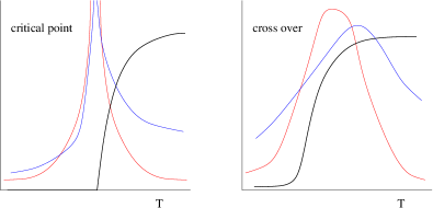
Figure 1: At a critical point order parameters change abruptly, and specific heats and susceptibilities may have singularities. The location of the singularity is unique. At a crossover there are no singularities. The order parameters may have a large continuous change. It is possible that specific heats and susceptibilities peak as the temperature changes. The locations of maximum slope of the order parameter, or the peaks of susceptibilities, generally depend on the observable chosen.

As the temperature of the vacuum is raised, keeping the baryon number and charge densities at zero, the condensate changes to a very small value, proportional to the quark mass. From thermodynamic arguments, models, and lattice QCD computations it is known that the change is gradual (see Figure 1). One may try to characterize a temperature where this crossover happens, but it is a conventional number [2]. The crossover temperature, $T_{c}$, depends upon which physical quantity is examined, but it is perfectly well-defined after a choice is made We make the choice that $T_{c}$ is given by the peak of the Polyakov loop susceptibility.

The quark number for each of the $N_{f}$ flavours is conserved. For the study of the phase diagram we need to keep in mind the up and down quark numbers (or, equivalently, the baryon number and the net isospin). A grand-canonical ensemble for QCD would then need two chemical potentials, $\mu_{u}$ and $\mu_{d}$ (or $\mu_{B}$ and $\mu_{I}$), and the temperature $T$: so the phase diagram is three dimensional. As a first approximation one treats the up and down quark masses to be equal, and examines the phase diagram in the two dimensional slice with $T$ and $\mu_{B}$ [3], and independently, of that in $T$ and $\mu_{I}$ [4]. There has been little study of the more complete (and complicated) phase diagram [5].

The phase diagram in $T$ and $\mu_{B}$ for small $\mu_{B}$ and non-zero light quark mass (see Figure 2) was first investigated in [3]. At small $\mu_{B}$ the states of QCD are distinguished by the value of the chiral condensate. In the low $T$ state it is large, but becomes small at $T>T_{c}$. At sufficiently high $T$ the dependence of the condensate on $\mu_{B}$ is computable, and shows a gradual variation. However, various arguments lead to the expectation that at low $T$ as one changes $\mu_{B}$ there is a first order phase transition signalled by an abrupt change in the condensate. The thermodynamic Gibbs’ phase rule [6] then tells us that the phase diagram has a line of first order transition. As we already discussed, this cannot hit the $\mu_{B}=0$ axis or rise to $T\to\infty$. So it must end somewhere. The end point is a second order phase transition, called the QCD critical point.

The actual location of the curve of first order phase transition curve and the critical end point can only be predicted by a non-perturbative computation, i.e., through lattice QCD simulations [7]. However, a computation at finite $\mu_{B}$ requires an extension of known techniques because of a technical problem known as the fermion sign problem. Many such methods have been proposed, and many are being explored [7]. It would be fair to say that developing such techniques is one of the most active areas in lattice gauge theory today.

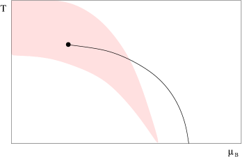
Figure 2: The phase diagram of QCD in the $T$-$\mu_{B}$ plane as seen with the chiral condensate [3]. A line of first order phase transitions (black line) ends in the QCD critical point (black dot). The fireball produced in a heavy-ion collision lives in a track within the shaded domain. The lower edge of this domain is called the freezeout curve. The domain is traced out by tracks of the history of the fireball as the collider energy changes. For small energies, the domain ends at $T=0$ and a chemical potential corresponding to nuclear matter. As the energy increases, the domain moves to small $\mu_{B}$. The logic of the beam energy scan is that this domain is likely to include the QCD critical point.

Till now extensive computations in QCD with varying lattice cutoffs, spatial volumes and quark masses has been possible using only one particular method, involving the Taylor expansion of the pressure in powers of $\mu_{B}$. As a result the information available until now is fairly limited, and one would hope that the future brings alternative computational schemes. The current best estimate of the location of the critical point is [8]

$$T^{E}\simeq(0.94\pm 0.01)T_{c}\qquad{\rm and}\qquad\mu_{B}^{E}\simeq(1.68\pm 0.06)T^{E}.$$ (1)

Methods have also been developed to compute the equation of state, the bulk compressibility, and the speed of sound in several parts of the phase diagram [8].

Two more aspects of the phase diagram of QCD are interesting, but cannot be described here. One is the temperature dependence of the axial anomaly. This has been keenly investigated in recent years [9]. The other is the phase diagram of QCD in a strong and constant external magnetic field. This has also generated much work recently [10].

3 General conditions in heavy-ion collisions

I turn now to heavy-ion collisions, which is the experimental system that can test the computations we discussed briefly in the previous section. In this section I touch upon three related questions: whether thermal matter is produced, what its flavour content is likely to be, and how one can control the energy content of this matter.

The object of study in heavy-ion collisions is the (hopefully) thermalized matter in the final state. In high energy colliders matter is always formed. In sufficiently hard pp collisions, for example at the LHC, even soft physics contains enough energy to create W/Z bosons, not to speak of hadrons. The mere production of large amounts of hadronic matter is not of interest. What we need to know is whether this matter re-interacts with sufficient strength to thermalize. In the language of particle physics this is about final state effects.

In order to understand the time scales involved it is sufficient to run through a simple kinetic theory argument. Let the two-body scattering cross section be $\sigma$. Taking the number density of particles in the final state to be $n$, one can write the mean free path as

$$\lambda\propto(n\sigma)^{-1},$$ (2)

If the dimensionless number $1/(\lambda\sqrt[3]{n})=\sigma/n^{2/3}={\cal O}(1)$ then the mean free path is of the same order as the mean separation between particles. In this case, final state collisions are numerous, and matter may come into local thermal equilibrium.

When $\sqrt{S}\simeq 20$ GeV, we know that jets are rare. As a result, we can take the final state particles to be hadrons, so that $\sigma\simeq 40$ mb. In this case $n\geq 5$/fm³ may be sufficient for the final state to thermalize. This number density cannot be reached in collisions of protons. However, heavy-ion collisions increases $n$ by some power of $A$, so heavy-ion collisions at this energy may thermalize. At the LHC, $n$ is large, so thermalization is easier. Even high multiplicity pp collisions may then thermalize. The thermalized system arising from these collisions is the fireball which is the object of study in heavy-ion collisions.

This treatment is sufficient for building intuition, but a quantitative analysis of thermalization is more complex. The rapid expansion of the fireball implies that simple kinetic theory does not suffice, and the theoretical framework becomes more complex. Some relevant references are collected here [11].

The flavour content of the fireball is needed in many analyses. Again, simple arguments are sufficient to gain a quick intuition about this. The flavour quantum numbers of the incoming hadrons are essentially contained in hard (valence) quarks. At large $\sqrt{S}$, the asymptotic freedom of QCD guarantees that our intuition about Rutherford scattering holds, and these valence quarks do not undergo large angle scattering. As a result, the incoming quantum numbers are mostly carried forward into the fragmentation region. In terms of the pseudo-rapidity

$$\eta=\frac{1}{2}\log\tan\theta,$$ (3)

(where $\theta$ is the scattering angle) the fragmentation region is the region of large $|\eta|$, and is called so because (classically) one finds the unscattered fragments of the initial particles here.

Although the valence partons individually contain large momenta, there are only three of them in a baryon. Soft (sea) partons are much more numerous. As a result, quite a significant fraction of the energy is carried by all the soft partons together. These generally scatter by large angles and so stay in the central rapidity region (i.e., the region with $|\eta|\simeq 1$). If this matter approximately thermalizes, then it makes the fireball which is the object of heavy-ion studies. The net-baryon and flavour content is small, the energy content increases with $\sqrt{S}$. At high energies the central and fragmentation regions are expected to be well separated, i.e., one expects few hadrons in the intermediate region between them.

At $\sqrt{S}\simeq$1–10 GeV, baryon interactions cannot be analyzed in terms of quarks. In this regime the fireball may contain baryon and other flavour quantum numbers. The distinction between fireball (central) and fragmentation region may be weak.

In the collision of point-like particles in quantum theory, the observables are the number of particles (or energy-momentum) hitting the detector at any angle $\theta$. The only control parameter is the center of mass energy, $\sqrt{S}$. In collisions of extended objects, there is another control parameter: the impact parameter, $b$. This measures the separation between the centers (geometrical centers, centers of energy) of the colliding objects. However, $b$ cannot directly be measured in an experiment.

Figure 3: The fraction of the total cross section can be used to define centrality classes. Different models of nuclear densities will map a centrality class to different impact parameter ranges.

Instead we perform the following analysis. The total nucleus-nucleus cross section depends only on the energy, so one has

$$\sigma(S)=\int_{0}^{\infty}db\frac{d\sigma(S)}{db}.$$ (4)

Since cross sections are non-negative, the fractional cross section

$$f(S,b)=\frac{1}{\sigma(S)}\int_{b}^{\infty}dB\frac{d\sigma(S)}{dB},$$

decreases monotonically as $b$ increases from zero to infinity (see Figure 3). As a result, an experimentally determined histogram of $f$ would determine $b$ uniquely, provided one knows the functional form of $f(\sqrt{S},B)$. This is not yet computable from QCD, so one has to make models.

The simplest, and oldest, model is called the Glauber model. In this, one assumes that the nucleus-nucleus collision is described by independent nucleon-nucleon collisions. The nucleons are distributed in each nucleus according to the density determined by low-energy electron nucleus collisions. Models which incorporate more phenomenology have also been developed; see [12] for more information. It has been realized in recent years that the lumpy distribution of nucleons in the initial state (see Figure 4) cannot always be averaged over, but must be taken into account in these models.

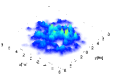
Figure 4: Transverse energy profiles, 0.2 fm after the collision, in three models of initial states [13]. The coarse-grained average of these distributions should give the nuclear density known through low-energy experiments. These relativistic experiments capture the quantum fluctuations in the initial nuclear wave-function.

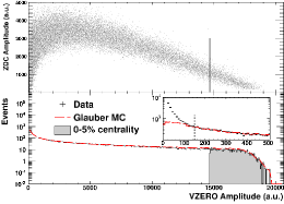
Figure 5: One of the definitions of centrality used by the ALICE collaboration [14] uses the histogram of measurements in the VZERO module. The experiment determines its correlation with the energy deposition in the ZDC.

As one sees, the connection between the impact parameter and the percent of total cross section is indirect and model dependent. Also, when one realizes that the positions of nucleons inside the nuclei fluctuate from one event to another, it is clear that the notion of an impact parameter, and even the size and shape of a nucleus, are merely averaged quantities. For experimental purposes what is necessary is to classify events according to the degree of centrality. For this it is enough to define centrality by any measure which changes monotonically with $b$; for example, by multiplicity, zero degree calorimetry, etc.. Care is needed to relate these measures to each other through careful analysis of the data. One such analysis is shown in Figure 5.

4 Hard probes

One thinks of the LHC as an arena of hard QCD, i.e., of processes which convert the partons contained in protons into jets, heavy quarks, W/Z bosons, hard $\gamma$, H and so on. The typical momentum scale in these processes is of the order $Q\simeq\langle x\rangle\sqrt{S}\simeq 500$ GeV. Final state interactions are suppressed in pp collisions because of two reasons. Firstly, the dense hadronic debris are separated from probes by large angles, $\Delta\eta$. Secondly, the energy scale of any remaining hadronic activity in the central rapidity region is small: $\langle E_{T}\rangle\simeq\Lambda_{\scriptscriptstyle QCD}\simeq 0.3$ GeV.

In heavy-ion collisions, the first argument can still be supported. However, the second argument may fail if the number density of particles, $n$, is large enough. Let us make an estimate by assuming, as before, that $n=5/{\rm fm\/}^{3}$. We know that the actual value of $n$ at the LHC is larger, so our argument will be overly conservative. Assume that the jet cone has radius $R=0.2$, and that it travels about $\ell=10$ fm through the fireball of soft particles. Then the net energy in the soft hadrons it can interact with is

$${\cal E}\simeq\langle E_{T}\rangle nR\ell^{3}\simeq 300{\rm\ GeV\/},$$ (5)

where we have made a conservative estimate that the average transverse energy of the particles is $\langle E_{T}\rangle\simeq 0.3$ GeV. Since this is comparable with the initial energy, final state interactions become important. An interesting consequence which we discuss here is jet quenching.

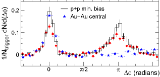
Figure 6: Comparison of two-particle azimuthal distributions for central d+Au collisions (circles) to those seen in p+p (histogram) and Au+Au collisions (stars). The respective pedestals have been subtracted.

When a jet evolves through a medium, interactions and radiation would tend to deplete its energy [15]. This simple idea is called jet quenching. The basic fact of jet quenching was beautifully demonstrated by the STAR collaboration in BNL [16] in the plot given above. At $\sqrt{S}=200$ GeV jets are not very well developed, and one must use high-$p_{\scriptscriptstyle T}$ hadrons as proxies. STAR triggered on events where there is a high-$p_{\scriptscriptstyle T}$ hadron, and looked at the angular distribution of the next highest-$p_{\scriptscriptstyle T}$ hadron. In p+p collisions they found a peak 180 degrees away (see Figure 6). If the trigger hadron can be assumed to come from a jet, then the backward peak comes from an away-side jet which balances the momentum. This was also seen in d+Au collisions, thus demonstrating that initial state parton effects in heavy nuclei do not wash away this peak. In Au+Au collisions they found no peak in the backward direction: implying that the away-side jet is hugely quenched.

A measure of the quenching is provided by a comparison of the number of jets of a given momentum in heavy-ion and proton collisions

$$R_{AA}(b,y,p_{\scriptscriptstyle T})=\frac{1}{T_{AA}(b)}\frac{d^{3}N_{AA}}{dbdydp_{\scriptscriptstyle T}}\left(\frac{d^{2}N_{pp}}{dydp_{\scriptscriptstyle T}}\right)^{-1}\,.$$ (6)

Here $T_{AA}$ is an estimate of the number of proton pairs interacting in AA collisions, and is usually extracted from a model, e.g., the Glauber model. The numerator depends on collision centrality whereas the denominator does not. Energy is tremendously more likely to flow from the jet into the low-momentum particles in the medium (computations reveal this in phase space factors). As a result, one would generally expect $R_{AA}$ to be less than unity.

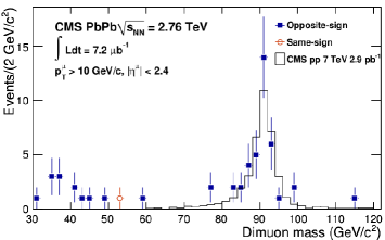
Figure 7: The first attempt to constrain $T_{AA}$ from experiment.

Since a basic input into jet-quenching is $T_{AA}$, it is important to constrain this through experiment. The production of high-$p_{\scriptscriptstyle T}$ photons or W/Z bosons provides this calibration. Since the vector bosons have no strong interactions, the comparison of semi-inclusive single boson production cross sections in pp and AA cross sections can directly measure $T_{AA}$. One of the first attempts [17] to constrain this is shown in Figure 7. Small isospin corrections, shadowing, and initial re-scattering effects must also be taken into account more accurately in order to improve these constraints.

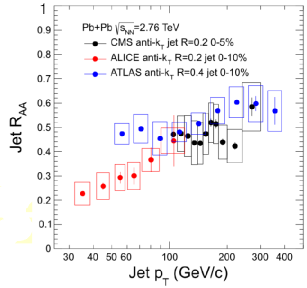
Figure 8: A recent compilation of data on $R_{AA}$ [18].

From the observations of $R_{AA}$ (see Figure 8) one can extract a measure of the $p_{T}$ change of the jet per unit distance travelled within the plasma:

$$\hat{q}=\frac{1}{L}\int\frac{d^{2}p_{T}}{(2\pi)^{2}}\,p_{T}^{2}\,P(p_{T},L).$$

Most attempts to extract this from data give $\hat{q}\simeq$ 1–2 GeV²/fm, i.e., in the range of interest, $\hat{q}/T^{3}\simeq$4–5. One should be able to extract this number for QCD, but it turns out to be a vexing problem. There are two main methods to handle problems in QCD: perturbative QCD is used to compute processes where all momenta involved are large, and lattice QCD provides a tractable computational method when all momenta are small. Jet quenching couples a large momentum object (the jet) to low-momentum objects (the medium). Nevertheless there have been attempts to compute this in QCD using weak-coupling expansions [19] or, more recently, lattice QCD [20]. There are also computations in cousins of QCD which have ${\cal N}=4$ supersymmetry in the limit of large $N_{c}$ [21].

$R_{AA}$ is just the simplest of experimental variables which can be constructed. In order to understand how the medium steals energy and momentum from the jet one should also understand medium modification of rapidity and angular correlation, momentum imbalance between reconstructed jets, fragmentation functions, and jet substructure.

5 Flow

Once the fireball reaches local thermal equilibrium a much slower process begins of transport of energy, momentum, and other conserved quantities through the fireball. This is the hydrodynamic regime [22]. Tests of hydrodynamics involve the study of quantities which are called flow coefficients [23]. In order to understand what these are, we need to think again about the geometry and kinematics of the collisions.

In the collision of point-like particles, there is a rotational symmetry around the beam axis. As a result, cross sections or particle production rates depend only on the scattering angle $\theta$ (or equivalently, on $\eta$ or the rapidity $y$) and the transverse momentum, $p_{\scriptscriptstyle T}$. Kinematically, there is only one initial vector in the center of mass (CM) frame of the problem, the initial momentum $\mathbf{k}$ of one of the particles (the other particle has momentum $-\mathbf{k}$). Final state momenta see only the angle from $\mathbf{k}$, which is $\theta$, and the transverse projection $p_{\scriptscriptstyle T}$.

In heavy-ion collisions, there is a second initial vector: $\mathbf{b}$, which is the line between the centers of the nuclei. The existence of such a vector, not collinear with $\mathbf{k}$, means that the azimuthal symmetry around $\mathbf{k}$ is broken in the initial state, and final state momentum distributions may depend on angles the final momentum makes with both $\mathbf{k}$ and $\mathbf{b}$ as well as $p_{\scriptscriptstyle T}$. Conventionally, these distributions are given in terms of $\eta$, $p_{\scriptscriptstyle T}$, and the azimuthal angle $\phi$. The two vectors $\mathbf{k}$ and $\mathbf{b}$ lie on a plane which is called the reaction plane. This breaking of cylindrical symmetry also occurs in proton-nucleus collisions, since the proton can meet the nucleus with a non-vanishing impact parameter. In very high energy collisions, the increasing proton-proton cross section implies that the swollen protons can also be treated similarly. One may already be seeing such effects in the sample of extreme high multiplicity events in pp collisions at the LHC.

The flow coefficients are the Fourier transforms of velocity distributions with respect to $\phi$ [24]. The $n$-th Fourier coefficient is denoted by the symbol $v_{n}$. These are normally taken at $y=0$ not only because of the limited rapidity coverage of heavy-ion detectors, but also because one expects the fireball to be well-separated from the fragmentation region. Nevertheless, studying the rapidity dependence of flow coefficients is of some interest. The study of the $k_{\scriptscriptstyle T}$ dependence of the $v_{n}$ is of great interest.

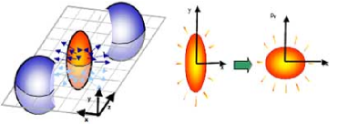
Figure 9: The geometry of elliptic flow.

Clearly, the reaction plane in different collisions can rotate around the beam axis, so single particle distributions will recover azimuthal symmetry when averaged over events. Although the overall orientation of the reaction plane is forgotten on the average, the relative angles between two particles remembers the difference from the reaction plane. So, in order to see the flow coefficients one has to construct the angular correlations of two or more particles.

In the collision of symmetric nuclei, $\mathbf{b}$ and $-\mathbf{b}$ seem to be completely equivalent. As a result the two sides of the reaction plane seem to be completely symmetric. This implies that only the even flow coefficients, $v_{2}$, $v_{4}$, etc., are non-vanishing (elliptic flow is the name given to $v_{2}$). However, when one studies the flow event-by-event (E/E) one has to take into account the fact that the positions of nucleons inside the nuclei may fluctuate. Then there may be more nucleons on one side of the plane, so breaking this orientational symmetry around the reaction plane, as a result of which odd harmonics may exist. Currently there are studies of the directed flow $v_{1}$, triangular flow $v_{3}$, and even the coefficient $v_{5}$. The flow coefficients yield a combination of information on the initial state and the evolution of fireball. E/E fluctuations of flow coefficients yield more refined information on the initial state [25]

It is claimed that the observations of $v_{2}$ imply the formation of locally thermalized matter in heavy-ion collisions. Although this argument is technical it is easy to understand this intuitively. In the off-center collisions of nuclei the colliding region is a pellet. Particles formed in the initial collisions have distributions which have positional anisotropy, $\epsilon_{n}$, the pellet being long in one direction (see Figure 9). The generation of $v_{n}$ involves transforming $\epsilon_{n}$ into momentum anisotropy. This is impossible unless there is hadronic re-scattering. Also, the measurements of $v_{2}$ show that the momentum is larger in the direction in which the original position distribution was squeezed. This is hydrodynamic flow, since that is driven by pressure gradients, and the gradients in the shorter direction are larger.

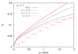
Figure 10: Predictions for elliptic flow from ideal hydrodynamics compared to data. See the text for a discussion.

The technical question here is how well does hydrodynamics explain the observed $v_{2}$. Ideal hydrodynamics, i.e., hydrodynamics without dissipation, is a toy model which is often used to understand general features of data. This already come within a factor two of the data, and shows the same $p_{\scriptscriptstyle T}$ dependence as the observations (see Figure 10). It also fails in the “right” direction, in that it over-estimates $v_{2}$. Dissipation would clearly reduce the predictions, and bring it closer to observations [26]. One of the first results (Dusling and Teaney in [26]) is shown in the figure. Intense work continues to be done in understanding the implications of the data and the constraints from QCD [27].

6 Chemical composition of the final state

The most easily observed quantities have to do with the final state. The basic observables are the spectra of identified particles. The multiplicity of each type of particle, $\pi^{\pm}$, $K^{\pm}$, etc., is called its yield. This is the integral over the spectrum. Relative yields of hadrons is the outcome of hadron chemistry, i.e., inelastic re-scattering in the final state. Examples are,

$$p+\pi^{-}\leftrightarrow n+\pi^{0},\qquad p+\pi^{-}\leftrightarrow\Lambda+K^{0},$$ (7)

The rates of such predictions determine whether hadron chemistry comes to chemical equilibrium.

As the fireball evolves, eventually mean-free paths or relaxation times become comparable to the size or expansion rate. When this happens, local thermal equilibrium can no longer be maintained, and hydrodynamics cannot be supported. Then the components of the fireball are said to freeze out. In principle freeze out could occur either before the fireball cools into hadrons or after. Under normal circumstances, i.e., if the thermal history of the fireball does not take it near a phase transition, then it seems to freeze out in the hadronic phase. This implies that the later stages of hydrodynamics require the equation of state of a hadronic fluid. Since hadrons are massive, inelastic collisions, i.e.those which change the particle content of the fireball, require larger energies than elastic collisions. As a result, chemical freezeout, i.e., fixing of the hadron content of the fireball, may occur earlier than kinetic freezeout, i.e., fixing of the phase space distribution of hadrons.

In the fireball the particles interact strongly enough that a temperature is maintained. However, at freeze out the interactions stop abruptly. So all hadrons emitted by the fireball at freeze out can be assumed to be an ideal gas of particles coming from a source whose temperature is set at the freeze out. This simple approximation, which goes by the name of the hadron resonance gas model has had remarkable phenomenological success [28]. However, recent measurements at the LHC (ALICE collaboration [28]) and a more careful look at RHIC results shows interesting discrepancies which imply that this model needs to be improved.

At early times, the fireball is a reactive fluid whose description requires coupling of hydrodynamics with diffusion and flavour chemistry. The reaction rates depend on local densities as well as rates of mixing due to fluid movement, known as advection, as well as diffusion. In order to make quantitative predictions, one must first understand whether advection or diffusion is more important in bringing reactants together. This is controlled by Peclet’s number

$${\rm Pe\/}=\frac{Lv}{D}=\frac{Lv}{\xi c_{s}}={\rm Kn\/}\,M,$$ (8)

where $L$ is a typical macroscopic distance within the fireball over which we wish to compare advection and diffusion, $v$ a typical flow velocity, $\xi$ is a typical density-density correlation length and $c_{s}$ is the speed of sound. The diffusion constant, $D\simeq\xi c_{s}$. We have also used the notation for the Mach number of the flow, $M=v/c_{s}$, and the Knudsen number, ${\rm Kn\/}=L/\xi$. When ${\rm Pe\/}\ll 1$ diffusion is more rapid than advection; when ${\rm Pe\/}\gg 1$ advection is more rapid [29].

Peclet’s number defines a new length scale in the fireball, this is the scale at which advection and diffusion become comparable—

$$L\simeq\frac{\xi}{M}.$$ (9)

Since longitudinal flow has $M\leq\sqrt{3}$, then taking $\xi$ to be approximately the Compton wavelength of a particle, we find that for baryons, $L\simeq 0.3$ fm and for strange particles, $L\simeq 0.5$ fm. This implies that advection may be important in chemical processes occurring in the early stages of the evolution of the fireball, but over most of its history, the availability of reactants is governed by diffusion.

Once the reactants have been brought together we can ask whether one or the other reaction channel is available. If the reactions are slower than the time scale of transport, then we may consider the fireball to be constantly stirred. It is then enough to examine chemical rate equations. In this approximation, a toy model which takes into account only pion and nucleon reactions is:

$$\dot{p} = -\gamma(p\pi^{0}-n\pi^{+})-\gamma^{\prime}(p\pi^{-}-n\pi^{0})+\cdots,$$

$$\dot{n} = \gamma(p\pi^{0}-n\pi^{+})+\gamma^{\prime}(p\pi^{-}-n\pi^{0})+\cdots,$$

$$\dot{\pi}^{0} = -\gamma(p\pi^{0}-n\pi^{+})+\gamma^{\prime}(p\pi^{-}-n\pi^{0})+\cdots,$$

$$\dot{\pi}^{+} = \gamma(p\pi^{0}-n\pi^{+})+\cdots,$$

$$\dot{\pi}^{-} = -\gamma^{\prime}(p\pi^{-}-n\pi^{0})+\cdots.$$

Here the label for a particle denotes the density of that particle. The rate constants $\gamma$ and $\gamma^{\prime}$ can be deduced from experimental measurements of cross sections. The equilibrium concentrations are given by

$$\frac{p}{n}=\frac{\pi^{+}}{\pi^{0}}=\frac{\pi^{0}}{\pi^{-}}\quad(=\zeta),$$ (10)

where $\zeta$ is the isospin fugacity. Since $\pi^{+}/\pi^{-}=\zeta^{2}$, if we set $\zeta\simeq 1$, then $\mu_{I}=T\log\zeta\simeq 0$. Even in this simple limit of a very rapidly stirred fireball, a more realistic model contains all possible reactions between many species of particles, of which many cross sections are unmeasured. As a result, a detailed model is out of reach and one must develop simplified models which catch as much of the physics as the state of the data justifies.

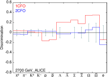
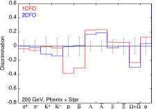
Figure 11: Comparison of model predictions with data in terms of the discriminant (model-data). The closer this is to zero, the better the model. The error bars show the error on the data and set the scale of what is acceptable mismatch between data and model. At all energies, 2CFO works better than 1CFO.

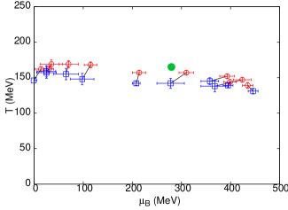
Figure 12: The freeze out points obtained in 2CFO (from Chatterjee et al., [30]). The strange freezeout point is shown with circles, and the non-strange with squares. The two freeze out points at the same $\sqrt{S}$ are joined with a line. The large filled circle is the estimated location of the QCD critical point from lattice computations [8].

In order to set up such a model, we consider flavour changing reactions. Strangeness changing processes seem to naturally split into subgroups. Indirect transmutations of $K$ and $\pi$ involve strange baryons in reactions such as $\Omega^{-}+K^{+}\leftrightarrow\Xi^{0}+\pi^{0}$. These have very high activation thresholds. Direct transmutations can proceed through the strong interactions such as $K^{+}+K^{-}\leftrightarrow\pi^{+}+\pi^{-}$. These are OZI violating reactions; slower than generic strong-interaction cross sections. Direct transmutations through weak interactions are not of relevance in the context of heavy-ion collisions. As a result, there is no physics forcing $K$ and $\pi$ to freezeout together. However $K$ and $\phi$ are resonantly coupled, so they may freeze out together [30]. On the other hand, isospin changing processes (the model in eq. 6) require extremely low activation temperatures, and may persist till later.

One can capture this information into a HRG model with two freezeout points: one for the strange hadrons and $\phi$ (since this is resonantly coupled to the $K^{\pm}$ channel), another for non-strange hadrons. We could call this model 2CFO [30] in contrast with the usual HRG model with a single freeze out (1CFO). A comparison of measurements and best fit model predictions is shown in Figure 11.

Interestingly, the introduction of two freeze out points allows one to do away with some unphysical features of the freeze out model 1CFO. In most such models there is a mismatch between strange and non-strange baryon production, which is fixed by having a fugacity factor which changes the occupancy of strange hadrons. This factor cannot be justified within an ideal gas picture, nor does it vary smoothly or monotonically as $\sqrt{S}$ is changed. Such nuisance parameters no longer appear within the 2CFO scheme.

The success of the 2CFO scheme implies that as one introduces more of the hadron dynamics into the freezeout process, the ability to describe the data improves. This justifies our belief that a proper description of reactive transport should be able to give a good description of the final observed yields.

The freeze out temperatures and chemical potentials in 2CFO are shown in Figure 12. Also shown there is the position of the critical point of QCD determined in lattice studies [8]. The freeze out curves pass close to the QCD critical point, making it plausible that a study of the final state as one scans in $\sqrt{S}$ can reveal signals of this very interesting prediction of QCD. This is the rationale for the RHIC Beam Energy Scan (BES) program and for planned future experiments in GSI and JINR.

Experiments also measure the yields of heavy-quarkonia. In particular, the yield of the $\Upsilon$ family of mesons in AA collisions at LHC differs significantly from that in pp collisions at same $\sqrt{S}$. This is usually reported in terms of an $R_{AA}$ for the meson. Since the quark mass is large, $M\gg T\simeq\Lambda_{\scriptscriptstyle QCD}$, one may expect that the production of quarkonia is a hard process. However the binding energy is of the order of the temperature, $B\simeq T$, so we may expect large thermal effects as the cause of the change between AA and pp collisions [32].

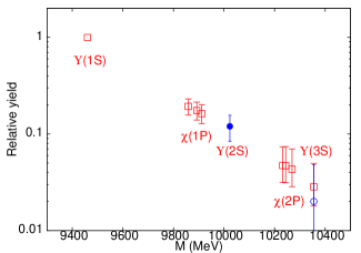
Figure 13: Measured (filled circles) and predicted (unfilled squares) suppression in the bottomonium family using a simple thermal model for freeze out [36].

Thermal lattice QCD computations show that the highest mass resonances, which are the least bound, are more easily disrupted at any given temperature [33]. This observation led to the formulation of a key observation called stepwise suppression, i.e., as $\sqrt{S}$ is increased $R_{AA}$ of the higher resonances drop below unity, roughly in the order of the binding energy [34]. If this works, then at a sufficiently high temperature it should be possible to use a thermal model to understand the relative yields of the $\Upsilon$ family of mesons using the variables

$$r[\Upsilon(n\ell)]=\frac{dN_{AA}^{\Upsilon(n\ell)}}{dydp_{T}}\left(\frac{dN_{AA}^{\Upsilon(1S)}}{dydp_{T}}\right)^{-1}.$$ (11)

The thermal model involves only a single parameter: the freeze out temperature of this family of mesons. The first data from the LHC [35] is fitted [36] well by

$$T_{f}^{\Upsilon}=222^{+28}_{-29}{\rm\ MeV}.$$ (12)

It will be interesting in future to see whether other members of the bottomonium family confirm this picture. Future data on $r[\Psi(n\ell)]$ will also provide useful tests. More detailed dynamical models [37] predict many more details of the kinematics of quarkonium suppression.

7 Fluctuations

Is the ensemble of heavy-ion collision events captured by a detector related to the ensembles required to study the thermodynamics of strong interactions?

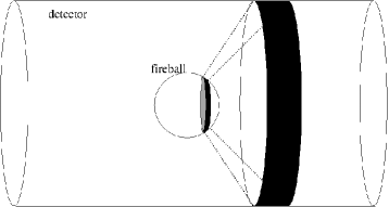
Figure 14: Selecting a volume in the fireball by selecting detector cuts works best when the momentum of particles in the volume are not totally arbitrary. Since hydrodynamics works, we know that in a small volume these momenta are aligned with the local fluid momentum, being smeared only by an amount of order $T$.

The least restrictive ensemble for the study of bulk matter is the microcanonical ensemble. All that this requires is that the energy of a system be fixed. In fact, since the fireball is well-separated from the spectators, one may expect a mapping between the collisions and microcanonical ensemble to be good. However there are two obstructions, neither of them absolute. The first is that the microcanonical ensemble requires the energy of each member of the ensemble to be the same. This is hard to ensure without more control on centrality fluctuations than is possible at present. Secondly, one needs $4\pi$-detectors to capture the entire energy of the fireball. Most detectors in use today miss a very large fraction of the energy.

So one must to try to map the ensemble of events recorded in the detector to either the canonical or a grand-canonical ensemble. The difference between these is that the system being studied must exchange either energy or material and energy (respectively) with a much larger system called a heat-bath. Since detectors accept particles from only a part of each fireball, one may be able to map the events on to a grand-canonical ensemble. Of course, thermal and chemical equilibrium is necessary in order to be able to do this.

We have already discussed the evidence that there is a degree of thermal and chemical equilibration at freeze out. So, if one observes a small part of the fireball, it may be possible to treat it in a grand-canonical ensemble where the rest of the fireball acts as the heat-bath. In order to make sure that the system (observed fraction of the fireball) is much smaller than the heat-bath (the unobserved fraction), one should use as small an angular coverage as possible while keeping the observed volume much larger than any intrinsic correlation volumes in the fireball (see Figure 14). If the acceptance in rapidity is $\Delta y$, $V_{s}$ is the size of the system, and $V_{b}$ is the volume of the heat-bath, then

$$\frac{V_{s}}{V_{s}+V_{b}}=\frac{\Delta y}{2\log(\sqrt{S}/M_{p})}\,.$$ (13)

Taking $\Delta y=2$, one sees that $V_{b}/V_{s}$ is about 4.3 at the top RHIC energy of 200 GeV, and around 7.5 at $\sqrt{S}=5$ TeV. These may be acceptable numbers. However, at $\sqrt{S}=20$ GeV the ratio drops to 2, and by $\sqrt{S}=5$ GeV, the “heat-bath” is smaller than the “system”. In order to keep the ratio $V_{b}/V_{s}$ fixed, one has to decrease $\Delta y$ with the beam energy.

This may give rise to another problem, which is to keep the observed volume much larger than correlation lengths. If freezeout occurs at time $\tau_{f}$, then the acceptance region, $\Delta y$, corresponds approximately to a distance $\Delta x=\tau_{f}\sinh(\Delta y)$. As long as correlation lengths are linear in the inverse freezeout temperature $1/T_{f}$, it is interesting to examine

$$\Delta xT_{f}=(\tau_{f}T_{f})\sinh\left(\frac{2\log\sqrt{S}}{1+V_{b}/V_{s}}\right).$$ (14)

If one wants $V_{b}/V_{s}\simeq 4$ at $\sqrt{S}=5$, where $T_{f}\simeq 145$ MeV, and one takes $\tau_{f}\simeq 5$ fm, then one finds $\Delta xT_{f}\simeq 2.5$. This is a reasonable number, but it implies that $\Delta y=0.65$ at this energy. Such a small acceptance window may cause statistics to drop significantly. However, for $\sqrt{S}\geq 20$ GeV, there is a good possibility that all these constraints may be satisfied simultaneously. Of course, if correlation lengths become very large at some $\sqrt{S}$ then all these arguments fail, and the system cannot be treated as being in equilibrium.

Conserved quantities, such as the net particle number or energy, can change by transport across the boundary of the system. As a result, energy and net particle numbers fluctuate in grand-canonical thermodynamics. These fluctuations can now be mapped into E/E fluctuations. They were first discussed and suggested as probes of the phase structure of QCD in [38]. The experimental variables which allow a direct comparison of QCD predictions with data were first discovered in [39], and the first lattice QCD predictions were made in [40].

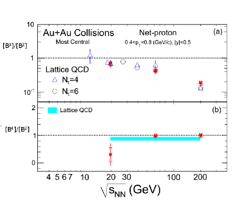
Figure 15: A comparison of data on fluctuations of net proton number in the STAR experiment with the lattice QCD computations of [40] from [43].

The existence of fluctuations means that the baryon number or energy of an ensemble is not a fixed quantity, but has a probability distribution. Such a distribution is characterized by the cumulants, $[B^{n}]$, which are defined as the Taylor coefficients of the logarithm of the Laplace transform of the distribution, $P(B)$, of the baryon number—

$$\log\left[\int\,dB\,P(B)\,{\rm e}^{-sB}\right]=\sum_{n=1}^{\infty}[B^{n}]\frac{(-s)^{n}}{n!}$$ (15)

The cumulants are related to the Taylor coefficients of the expansion of the free energy [39] in terms of $\mu_{B}$ simply as

$$[B^{n}]=V_{s}\chi^{(n)}(T_{f},\mu_{B}^{f})\,T_{f}^{n-1},$$ (16)

where $\chi^{(n)}(T,\mu_{B})$ are generalized quark number susceptibilities ($\chi^{(1)}$ is the baryon density) [41]. As a result, ratios of the cumulants are independent of the factor $V_{s}$. These ratios depend on the ratios of the dimensionless quantities $\chi^{(n)}(T_{f},\mu_{B}^{f})T_{f}^{n-4}$, which can be computed in lattice QCD, as demonstrated in [40]. Similar ratios were also discussed in [42].

Since $T_{f}$ and $\mu_{B}^{f}$ was already known from the analysis of yields, the experimental data could be compared to the lattice computation [43]. This comparison is reproduced in Figure 15. The remarkably good agreement has led to subsequent attempts to refine the comparison. These include following up the suggestions in [40] that the comparison could yield a measurement of $T_{c}$ given $T_{f}$ and $\mu_{B}^{f}$ [44] or the determination of $T_{f}$ and $\mu_{B}^{f}$ given $T_{c}$ [45]. There has also been a lot of work on various corrections which may need to be applied to the experimental data before comparing with predictions [46]. There is also sustained interest in fluid dynamical effects [29, 47]. In the meanwhile, much new experimental data has been added from the RHIC Beam Energy Scan (BES) [48]. A BES-II is expected shortly.

The long-term goal of the study of fluctuations is to understand the evolution of fluctuations along the freeze-out curve traced by changing the beam energy [39]. At higher energies one sees preliminary agreement between lattice predictions and experimental observations. This agreement is expected to break down in the vicinity of the QCD critical point because correlation lengths and relaxation times grow [49]. At lower energies one might expect a return to roughly thermal behaviour, although extracting this is fraught with theoretical and experimental challenges. The BES program aims to locate and study bulk matter near the QCD critical point.

8 Acknowledgement

I would like to thank the organizers of AEPSHEP 2014 for building a very stimulating scientific program, and for the wonderful local organization. It was a pleasure to lecture in this school. I would like to thank the Kavli Institute for Theoretical Physics China for hospitality during a part of the time that this manuscript was in preparation. I would like to thank Bedangadas Mohanty and Rishi Sharma for their helpful comments on the manuscript.

References

- [1] S. Weinberg, Quantum Theory of Fields: Modern Applications, Vol II, Cambridge University Press (2010) Cambridge, Great Britain.
- [2] R. D. Pisarski and F. Wilczek, Phys. Rev. D 29 (1984) 338; Y. Aoki et al., Phys. Lett. B 643 (2006) 46 [hep-lat/0609068]; A. Bazavov et al., Phys. Rev. D 85 (2012) 054503 [arxiv:1111.1710].
- [3] J. Berges and K. Rajagopal, Nucl. Phys. B 538 (1999) 215 [hep-ph/9804233]; A. M. Halasz et al., Phys. Rev. D 58 (1998) 096007 [hep-ph/9804290].
- [4] D. T. Son and M. A. Stephanov, Phys. Rev. Lett. 86 (2001) 592 [hep-ph/0005225].
- [5] R. V. Gavai and S. Gupta, Phys. Rev. D 66 (2002) 094510 [hep-lat/0208019]; S. Gupta, arxiv:0712.0434.
- [6] L. D. Landau and E. M. Lifshitz, Course of Theoretical Physics: Statistical Physics, Vol 5, Butterworth-Heinemann (1980) Oxford, Great Britain.
- [7] Ph. de Forcrand, PoS LATTICE2009 (2009) 010 [arxiv:1005.0539]; S. Gupta, PoS LATTICE2010 (2010) 007 [arxiv:1101.0109]; L. Levkova, PoS LATTICE2011 (2011) 011 [arxiv:1201.1516]; G. Aarts, PoS LATTICE 2012 (2012) 017 [arxiv:1302.3028]; C. Gattringer, PoS LATTICE2013 (2014) 002 [arxiv:1401.7788].
- [8] R. V. Gavai and S. Gupta, Phys. Rev. D 71 (2005) 114014 [hep-lat/0412035]; R. V. Gavai and S. Gupta, Phys. Rev. D 78 (2008) 114503 [arxiv:0806.2233]; S. Datta et al., PoS LATTICE2013 (2014) 202; S. Gupta et al., Phys. Rev. D 90 (2014) 034001 [arxiv:1405.2206].
- [9] R. V. Gavai et al., Phys. Rev, D 77 (2008) 114506 [arxiv:0803.0182]; A. Bazavov et al., Phys. Rev, D 86 (2012) 094503 [arxiv:1205.3535]; C. Bonati et al., Phys. Rev. Lett. 110 (2013) 252003 [arxiv:1301.7640]; G. Cossu et al., Phys. Rev. D 87 (2013) 114514 [arxiv:1304.6145]; M. I. Buchoff et al., Phys. Rev. D 89 (2014) 054514 [arxiv:1309.4149]; T.-W. Chiu et al., PoS LATTICE2013 (2014) 165 [arxiv:1311.6220]; V. Dick et al., Phys. Rev. D 91 (2015) 094504 [arxiv:1502.06190].
- [10] M. D’Elia et al., Phys. Rev. D 82 (2010) 051501 [arxiv:1005.5365]; G. S. Bali et al., J. H. E. P. 1202 (2012) 044 [arxiv:1111.4956]; V. Skokov, Phys. Rev. D 85 (2012) 034026 [arxiv:1112.5137]; E.-M. Ilgenfritz et al.Phys. Rev. D 85 (2012) 114504 [arxiv:1203.3360]; F. Bruckmann et al., J. H. E. P. 1304 (2013) 112 [arxiv:1303.3972]; L. Levkova and C. De Tar, Phys. Rev. Lett. D 112 (2014) 012002 [arxiv:1309.1142]; C. Bonati et al.Phys. Rev. D 89 (2014) 054506 [arxiv:1310.8656]; G. S. Bali et al., J. H. E. P. 1408 (2014) 177 [arxiv:1406.0269];
- [11] R. Baier et al., Phys. Lett. B 502 (2001) 51 [hep-ph/0009237]; A. Dumitru et al., Phys. Rev. D 75 (2007) 025016 [hep-ph/0604149]; P. Romatschke and R. Venugopalan, Phys. Rev. D 74 (2006) 045011; Y. V. Kovchegov and A. Taliotis, Phys. Rev. C 76 (2007) 014905 [arxiv:0705.1234]; D. A. Teaney, arxiv:0905.2433; V. Balasubramanian et al., Phys. Rev. 84 (2011) 026010 [arxiv:1103.2683]; A. Kurkela and G. D. Moore, J. H. E. P. 1112 (2011) 044 [arxiv:1107:5050]; K. Fukushima and F. Gelis, Nucl. Phys. A 874 (2012) 108 [arxiv:1106.1396]; T. Epelbaum and F. Gelis, Nucl. Phys. A 872 (2011) 210 [arxiv:1107.0668]; J.-P. Blaizot et al., Nucl. Phys. A 873 (2012) 68 [arxiv: 1107.5296]; J. Berges et al., Phys. Rev. D 89 (2014) 7, 074011 [arxiv: 1303:5650].
- [12] N. Armesto et al., J. Phys. G 35 (2008) 054001 [arxiv:0711.0974]; B. Miller et al., Ann. Rev. Nucl. Part. Sci. 62 (2012) 361 [arxiv:1202.3233].
- [13] C. Gale et al., Phys. Rev. Lett. 110 (2013) 012302 [arxiv:1209.6330].
- [14] K. Aamodt et al., Phys. Rev. Lett. 105 (2010) 252301 [arxiv:1011.3916].
- [15] M. Gyulassy and M. Plümer, Phys. Lett. B 243 (1990) 432; X.-N. Wang and M. Gyulassy, Phys. Rev. Lett. 68 (1992) 1480.
- [16] STAR Collaboration, Phys. Rev. Lett. 91 (2003) 072304 [arxiv:nucl-ex/0306024]
- [17] S. Chatrchyan et al.(CMS Collaboration), Phys. Rev. Lett. 106 (2011) 212301 [arxiv:1102.5435].
- [18] Yan-Jie Lee, QM 2014: https://indico.cern.ch/ event/ 219436/ session/ 3/ contribution/ 728/ material/ slides/ 1.pdf
- [19] R. Baier et al., Phys. Lett. B 345 (1995) 277 [hep-ph/9411409]; P. B. Arnold et al., J. H. E. P. 0206 (2002) 030 [hep-ph/0204343]; G. Baym et al., Phys. Lett. B 644 (2007) 48 [hep-ph/0604209]; S. Peigne and A. V. Smilga, Phys. Usp. 52 (2009) 659 [arxiv:0810.5702]; S. Caron-Huot, Phys. Rev. D 79 (2009) 065039 [arxiv:0811.1603]. J. Ghiglieri and D. Teaney, arxiv:1502.03730.
- [20] A. Majumder, Phys. Rev. C 87 (2013) 034905 [arxiv:1202.5295]; X. Ji, Phys. Rev. Lett. 110 (2013) 262002 [arxiv:1305.1539]; M. Panero et al., Phys. Rev. Lett. 112 (2014) 162001 [arxiv:1307.5850]; M. Laine and A. Rothkopf, PoS LATTICE2013 (2013) 174 [arxiv:1310.2413].
- [21] H. Liu et al., Phys. Rev. Lett. 98 (2007) 182301 [hep-ph/0607062]; H. Liu et al., J. H. E. P. 0703 (2007) 066 [hep-ph/0612168]; J. Casalderrey-Solana and D. Teaney, J. H. E. P. 0704 (2007) 039 [hep-th/0701123]; Y. Hatta, E. Iancu and A. H. Mueller J. H. E. P. 0805 (2008) 037 [arxiv:0803.2481]; P. M. Chesler et al., Phys. Rev. D 79 (2009) 125015 [arxiv:0810.1985]; J. de Boer et al., J. H. E. P. 0907 (2009) 094 [arxiv:0812.5112].
- [22] J. D. Bjorken, Phys. Rev. D 27 (1983) 140.
- [23] J.-Y. Ollitrault, Phys. Rev. D 46 (1992) 229.
- [24] S. Voloshin and Y. Zhang, Z. Phys. C 70 (1996) 665 [hep-ph/9407282].
- [25] A. P. Mishra et al., Phys. Rev. C 81 (2010) 034903 [arxiv:0811.0292]; B. Alver and G. Roland, Phys. Rev. C 81 (2010) 054905 [arxiv:1003.0194]; D. Teaney and Li Yan, Phys. Rev. C 83 (2011) 064904 [arxiv:1010.1876].
- [26] H.J. Dresher et al., Phys. Rev./ C 76 (2007) 024905 [arxiv:0704.3553]; P. Romatschke and U. Romatschke, Phys. Rev. Lett. 99 (2007) 172301 [arxiv:0706.1522]; H. Song and U. W. Heinz, Phys. Lett. B 658 (2008) 279 [arxiv:0709.0742]. K. Dusling and D. Teaney, Phys. Rev. C 77 (2008) 034905 [arxiv:0710.5932]
- [27] M. Luzum and P. Romatschke, Phys. Rev. C 78 (2008) 034915 [arxiv:0804.4015]; G. Ferini et al., Phys. Lett. B 670 (2009) 325 [arxiv:0805.4814]; T. Hirano and Y. Nara, Phys. Rev. C 79 (2009) 064904 [arxiv:0904.4080]; K. Dusling et al., Phys. Rev. C 81 (2010) 034907 [arxiv:0909.0754]; B. Schenke et al., Phys. Rev. C 82 (2010) 014903 [arxiv:1004.1408]; H. Holopainen et al., Phys. Rev. C 83 (2011) 034901 [arxiv:1007.0368]; G.Y. Qin et al., Phys. Rev. C 82 (2010) 064903 [arxiv:1009.1847]; C. Shen et al., Phys. Rev. C 84 (2011) 044903 [arxiv:1105.3226]; P. Bozek, Phys. Rev. C 85 (2012) 034901 [arxiv:1110.6742]; M. Martinez et al., Phys. Rev. C 85 (2012) 064913 [arxiv:1204.1473]; D. Teaney and Li Yan, Phys. Rev. C 86 (2012) 044908 [arxiv:1206.1905]; STAR Collaboration, Phys. Rev. C 88 (2013) 014904 [arxiv:1301.2187]; CMS Collaboration, Phys. Lett. B 724 (2013) 213 [arxiv:1305.0609]; ATLAS Collaboration, J. H. E. P. 1311 (2013) 183 [arxiv:1305.2942]; ALICE Collaboration, Phys. Lett. B 726 (2013) 164 [arxiv:1307.3237].
- [28] J. Cleymans and K. Redlich, Phys. Rev. Lett. 81 (1998) 5284 [nucl-th/9808030]; Z.-W. Lin et al., Phys. Rev. C 72 (2005) 064901 [nucl-th/064901]; A. Andronic et al., Nucl. Phys. A 772 (2006) 167 [nucl-th/0511071]; F. Becattini et al., Phys. Rev. C73 (2006) 044905 [hep-ph/0511092]; NA49 Collaboration Phys. Rev. C 73 (2006) 044910; V. V. Begun et al., Phys. Rev. C 76 (2007) 024902 [nucl-th/0611075]; F. Becattini and J. Manninen, J. Phys. G 35 (2008) 104013 [arxiv:0805.0098]; STAR Collaboration, arxiv:1007.2613; M. Chojnacki et al., Comput. Phys. Commun. 183 (2012) 746 [arxiv:1102.0273]; ALICE Collaboration, Phys. Rev. C 88 (2013) 044910 [arxiv:1303.0737]; S. Borsanyi et al., Phys. Rev. Lett. 111 (2013) 062005 [arxiv:1305.5161].
- [29] R. S. Bhalerao and S. Gupta, Phys. Rev. C 79 (2009) 064901 [arxiv:0901.4677].
- [30] S. Chatterjee et al., Phys. Lett. B 727 (2013) 554 [arxiv:1306.2006]; K. A. Bugaev et al., Europhys. Lett. 104 (2013) 22002 [arxiv:1308.3594].
- [31] J. Steinheimer et al., Phys. Rev. Lett. 110 (2013) 042501 [arxiv:1203.5302]; F. Becattini et al.Phys. Rev. Lett. 111 (2013) 082302 [arxiv:1212.2431].
- [32] T. Matsui and H. Satz, Phys. Lett. B 178 (1986) 416.
- [33] M. Asakawa and T. Hatsuda, Phys. Rev. Lett. 92 (2004) 012001 [hep-lat/0308034]; S. Datta et al., Phys. Rev. D 69 (2004) 094507 [hep-lat/0312037].
- [34] F. Karsch et al., Phys. Lett. B 637 (2006) 75 [hep-ph/0512239]; H. Satz, Nucl. Phys. A 783 (2007) 249.
- [35] S. Chatrchyan et al.Phys. Rev. Lett. 109 (2012) 222301 [arxiv:1208.2826]; S. Chatrchyan et al.Phys. Rev. Lett. 107 (2011) 052302 [arxiv:1105.4894].
- [36] S. Gupta and R. Sharma, Phys. Rev. C 89 (2014) 057901 [arxiv:1401.2930].
- [37] N. Brambilla et al., Eur. Phys. J. C 71 (2011) 1534, and references therein.
- [38] M. A. Stephanov et al., Phys. Rev. Lett. 81 (1998) 4816 [hep-ph/9806219]; M. A. Stephanov et al., Phys. Rev. D 60 (1999) 114028 [hep-ph/9903292].
- [39] S. Gupta, PoS CPOD2009 (2009) 025 [arxiv:0909.4630]; S. Gupta, Prog. Theor. Phys. Suppl. 186 (2010) 440.
- [40] R. V. Gavai and S. Gupta, Phys. Lett. B 696 (2011) 459 [arxiv:1001.3796].
- [41] R. V. Gavai and S. Gupta, Phys. Rev. D 68 (2003) 034506 [hep-lat/0303013].
- [42] C. Athanasiou et al., Phys. Rev. D 82 (2010) 074008 [arxiv:1006.4636].
- [43] M. M. Aggarwal et al.(STAR Collaboration), Phys. Rev. Lett. 105 (2010) 022302 [arxiv:1004.4959].
- [44] S. Gupta et al., Science 332 (2011) 1525 [arxiv:1105.3934].
- [45] A. Bazavov et al., Phys. Rev. Lett. 109 (2012) 192302 [arxiv:1208.1220]; S. Borsanyi et al., Phys. Rev. Lett. 111 (2013) 062005 [arxiv:1305.5161].
- [46] E. S. Fraga et al., Phys. Rev. C 84 (2011) 011903 [arxiv:1104.3755]; M. Kitazawa and M. Asakawa Phys. Rev. C 85 (2012) 021901 [arxiv:1107.1412]; A. Bzdak etal, Phys. Rev. C 87 (2013) 014901 [arxiv:1203.4529]; M. Kitazawa and M. Asakawa Phys. Rev. C 86 (2012) 024904 [arxiv:1205.3292]; V. Skokov and B. Friman, Phys. Rev. C 88 (2013) 034911 [arxiv:1205.4756]; A. Bzdak and V. Koch, Phys. Rev. C 86 (2012) 044904 [arxiv:1206.4286]; X. Luo et al., J. Phys. G 40 (2013) 105104 [arxiv:1302.2332]; H. Ono et al., Phys. Rev. C 87 (2013) 041901 [arxiv:1303.3338]; P. Garg et al., Phys. Lett. B 726 (2013) 691 [arxiv:1304.7133]; A. Tang and G. Wang, Phys. Rev. C 88 (2013) 024905 [arxiv:1305.1392]; L. Chen et al., J. Phys. G 41 (2014) 105107 [arxiv:1312.0749]; A. Bzdak and V. Koch, Phys. Rev. C 91 (2015) 027901 [arxiv:1312.4574]; X. Luo et al., Nucl. Phys. A 931 (2014) 808 [arxiv:1408.0495]; M. Sakaida et al., Phys. Rev. C 90 2014) 064911 [arxiv:1409.6866].
- [47] M. A. Stephanov, Phys. Rev. D 81 (2010) 054012 [arxiv:0911.1772]; K. Xiao et al., Chin. Phys. C 35 (2011) 467; J. I. Kapusta and J. M. Torres-Rincon, Phys. Rev. C 86 (2012) 054911 [arxiv:1209.0675]; M. Kitazawa, arxiv: 1505.04349; S. Mukherjee et al., arxiv:1506.00645
- [48] X. Zhang (STAR Collaboration) Nucl. Phys. A 904-905 (2013) 543c; A. Sarkar (STAR Collaboration) PoS CPOD2013 (2013) 043; L. Adamczyk et al.(STAR Collaboration) Phys. Rev. Lett. 112 (2014) 032302 [arxiv:1309.5681]; L. Adamczyk et al.(STAR Collaboration) Phys. Rev. Lett. 113 (2014) 092301 [arxiv:1402.1558]; A. Adare et al.(PHENIX Collaboration) arxiv:1506.07834.
- [49] B. Berdnikov and K. Rajagopal, Phys. Rev. D 61 (2000) 105017 [hep-ph/9912274]; M. A. Stephanov, Phys. Rev. Lett. 102 (2009) 032301 [arxiv:0809.3450].