Abstract

In this paper, we consider multivariate response regression models with high dimensional predictor variables. One way to model the correlation among the response variables is through the low rank decomposition of the coefficient matrix, which has been considered by several papers for the high dimensional predictors. However, all these papers focus on the singular value decomposition of the coefficient matrix. Our target is the decomposition of the coefficient matrix which leads to the best lower rank approximation to the regression function, the signal part in the response. Given any rank, this decomposition has nearly the smallest expected prediction error among all approximations to the the coefficient matrix with the same rank. To estimate the decomposition, we formulate a penalized generalized eigenvalue problem to obtain the first matrix in the decomposition and then obtain the second one by a least squares method. In the high-dimensional setting, we establish the oracle inequalities for the estimates. Compared to the existing theoretical results, we have less restrictions on the distribution of the noise vector in each observation and allow correlations among its coordinates. Our theoretical results do not depend on the dimension of the multivariate response. Therefore, the dimension is arbitrary and can be larger than the sample size and the dimension of the predictor. Simulation studies and application to real data show that the proposed method has good prediction performance and is efficient in dimension reduction for various reduced rank models.

Keyword: multivariate regression; high dimensional predictors; signal extraction; dimension reduction; best lower rank approximation; oracle inequalities.

1 Introduction

In this paper, we consider multivariate response regression models with high dimensional predictor variables. Several methods have been proposed to estimate the coefficient matrix and select a common subset of explanatory variables. The sparse partial least square method (Chun and Keles, 2010) finds sparse linear combinations of the original predictors to maximize their covariance with response variables. Turlach et al. (2005), Similä and Tikka (2007), Peng et al. (2010), Chen and Huang (2012), Chen et al. (2012), and Bunea et al. (2012) estimate the coefficient matrix by minimizing the penalized (joint) residual sum of squares with different penalties. Similä and Tikka (2007) and Turlach et al. (2005) assume row sparsity of the coefficient matrix and use group-Lasso type penalties with $l_{2}$ or $l_{\infty}$ norm that treat each row of the regression coefficient matrix as a group. Peng et al. (2010) imposes both row-wise and element-wise sparsity on the coefficient matrix. In addition to the row-wise sparsity assumption, Chen and Huang (2012), Chen et al. (2012) and Bunea et al. (2012) make the reduced rank assumption on the regression coefficient matrix (Izenman, 1975; Reinsel and Velu, 1998). Under this assumption, Chen and Huang (2012) and Chen et al. (2012) aim to estimate the singular value decomposition (SVD) of the coefficient matrix. Chen and Huang (2012) specify the rank by the cross-validation method, and use a group-Lasso type penalty on the first matrix in the SVD of the coefficient matrix to achieve sparsity. Chen et al. (2012) pre-specifies the rank by existing methods as given in Anderson (2002), Camba-Mendez et al. (2003) or Bunea et al. (2011), and impose an adaptive-lasso type penalty. Bunea et al. (2012) penalizes on the rank sparsity and the variable sparsity simultaneously, and provides theoretical results in the high-dimensional settings.

We also assume the reduced-rank structure and the row-wise sparsity on the coefficient matrix. Instead of the SVD of the coefficient matrix, our target is the decomposition of the coefficient matrix which leads to the best lower rank approximation to the regression function, the product of the design matrix and the coefficient matrix. Given any rank, this decomposition has the smallest approximation error to the regression function and nearly the smallest expected prediction error among all approximations to the coefficient matrix with the same rank. Therefore, our proposed method is expected to have good prediction performance and be efficient in dimension reduction. To estimate this decomposition, we first propose a penalized generalized eigenvalue problem to obtain the first lower rank matrix in this decomposition, and then obtain the second by a least squares method. In the high-dimensional setting, we establish the oracle inequalities for the estimators of the lower rank matrices, the coefficient matrix and the estimated regression function, respectively. Bunea et al. (2012) provides the convergence rate of the estimate of the regression function under the assumption that the coordinates of the noise vector are identically independently distributed normal randoms variables. The convergence rate depends on the dimension of the multivariate response variable. In order that the convergence rate goes to zero, the increase of the dimension of the multivariate response variable has to be slower than the sample size. We make weaker assumption on the distribution of the noise vector and allow correlations among its coordinates. Our theoretical results do not depend on the dimension of the multivariate response. Therefore, the dimension of the multivariate response can be arbitrary and even larger than the sample size and the dimension of the predictor. Through simulation studies on the reduced rank models with various settings, we demonstrate that our method has competitive predictive ability and is efficient in dimension reduction.

The paper is organized as follows. In Section 2, we formulate the best lower rank approximation problem and establish its equivalence with a generalized eigenvalue problem. In Section 3, in the high dimensional settings, we propose sparse estimates of the decomposition and the coefficient matrix. We establish the oracle inequalities for the estimates. In Section 4, we discuss the choice of the number of components and tuning parameters. We conduct simulation studies and a case study in Sections 5 and 6, respectively, and summarize the paper with discussion in Section 7. All the proofs can be found in the supplementary material.

2 Signal extraction approach to multivariate regression (SiER)

We consider the following linear regression model with responses taking values in $\mathbf{R}^{q}$, where $q\geq 1$. Suppose that the $i$-th observation satisfies $\mathbf{y}_{i}=x_{i1}\boldsymbol{\beta}_{1}+x_{i2}\boldsymbol{\beta}_{2}+\cdots+x_{ip}\boldsymbol{\beta}_{p}+\boldsymbol{\varepsilon}_{i}$, $1\leq i\leq n$. Here $x_{ij}\in\mathbb{R}$ is the $i$-th observed value of the $j$-th predictor variable, $\mathbf{y}_{i}=({y}_{i1},{y}_{i2},\cdots,{y}_{iq})^{\rm T}\in\mathbb{R}^{q}$ and $\boldsymbol{\varepsilon}_{i}=({\varepsilon}_{i1},{\varepsilon}_{i2},\cdots,{\varepsilon}_{iq})^{\rm T}\in\mathbb{R}^{q}$ are the $i$-th observed response vector and the $i$-th noise vector, respectively, and each coefficient $\boldsymbol{\beta}_{j}=({\beta}_{j1},{\beta}_{j2},\cdots,{\beta}_{jq})^{\rm T}$, $j=1,\ldots,p$, is a $q$-dimensional vector. Let $\mathbf{x}_{i}=({x}_{i1},{x}_{i2},\cdots,{x}_{ip})^{\rm T}$ denote the $i$-th observation of the $p$-dimensional predictor vector, $\mathbf{Y}=[\mathbf{y}_{1},\cdots,\mathbf{y}_{n}]^{\rm T}$ the $n\times q$ response matrix, $\mathbf{X}=[\mathbf{x}_{1},\cdots,\mathbf{x}_{n}]^{\rm T}$ the $n\times p$ design matrix, $\mathcal{B}=[\boldsymbol{\beta}_{1},\cdots,\boldsymbol{\beta}_{p}]^{\rm T}$ the $p\times q$ coefficient matrix, and $\boldsymbol{\varepsilon}=[\boldsymbol{\varepsilon}_{1},\cdots,\boldsymbol{\varepsilon}_{n}]^{\rm T}$ the $n\times q$ random noise matrix, respectively. We assume that $\boldsymbol{\varepsilon}_{1},\cdots,\boldsymbol{\varepsilon}_{n}$, are i.i.d. random vectors with $E[\boldsymbol{\varepsilon}_{i}]=\mathbf{0}$. Correlations are allowed among coordinates of $\boldsymbol{\varepsilon}_{i}$, $1\leq i\leq n$. Throughout this paper, we will assume that $\mathbf{X}$ is nonrandom and the column means of $\mathbf{X}$ are all zeros, the same setting as in Bickel et al. (2009). Then the model can be written as

$$\mathbf{Y}=\mathbf{X}\mathcal{B}+\boldsymbol{\varepsilon}\;.$$ (2.1)

In this paper, we make the reduced-rank assumption, that is, the rank of $\mathcal{B}$, denoted by $K$, is small compared to $n$, $p$ and $q$. As the dimension of the subspace spanned by $\{\boldsymbol{\beta}_{1},\cdots,\boldsymbol{\beta}_{p}\}$ in $\mathbb{R}^{q}$ is equal to $K$, given any $K$ linearly independent vectors $\mathbf{w}_{1},\cdots,\mathbf{w}_{K}$ in this subspace, each coefficient vector $\boldsymbol{\beta}_{j}$ can be expressed as a linear combination of $\mathbf{w}_{1},\cdots,\mathbf{w}_{K}$. So we have the decomposition

$$\mathcal{B}=\mathbf{A}\mathbf{W}^{\rm T}=\boldsymbol{\alpha}_{1}\mathbf{w}_{1}^{\rm T}+\cdots+\boldsymbol{\alpha}_{K}\mathbf{w}_{K}^{\rm T},$$ (2.2)

where $\mathbf{A}=[\boldsymbol{\alpha}_{1},\cdots,\boldsymbol{\alpha}_{K}]$ and $\mathbf{W}=[\mathbf{w}_{1},\cdots,\mathbf{w}_{K}]$ are $p\times K$ and $q\times K$ matrices, respectively. There are infinitely many choices of $\mathbf{w}_{1},\cdots,\mathbf{w}_{K}$, hence the decomposition $\eqref{70001}$ is not unique. Chen and Huang (2012) and Chen et al. (2012) consider the SVD, $\mathcal{B}=\mathbf{U}\mathbf{D}\mathbf{V}^{\rm T}$, where $\mathbf{U}$ and $\mathbf{V}$ are $p\times K$ and $q\times K$ matrices with orthonormal columns, respectively, and $\mathbf{D}$ is a $K\times K$ nonnegative diagonal matrix. This SVD is a special case of $\eqref{70001}$ with

$$\mathbf{A}=\mathbf{U}\mathbf{D}\text{ and }\mathbf{W}=\mathbf{V}.$$ (2.3)

We will consider a different decomposition which leads to the best lower rank approximation to $\mathbf{X}\mathcal{B}$, the signal in $\mathbf{Y}$. Specifically, we want to find $\mathbf{A}$ and $\mathbf{W}$ such that for any $1\leq k\leq K$, we have

$$\|\mathbf{X}\mathcal{B}-\sum_{j=1}^{k}\mathbf{X}\boldsymbol{\alpha}_{j}\mathbf{w}_{j}^{\rm T}\|_{F}^{2}=\min_{\begin{subarray}{c}\mathbf{r}_{j}\in\mathbb{R}^{n},\mathbf{v}_{j}\in\mathbb{R}^{q},\\ 1\leq j\leq k\end{subarray}}\|\mathbf{X}\mathcal{B}-\sum_{j=1}^{k}\mathbf{r}_{j}\mathbf{v}_{j}^{\rm T}\|_{F}^{2},$$ (2.4)

where $\|\cdot\|_{F}$ is the Frobenius norm and is define as $\|\mathbf{M}\|_{F}=\sqrt{\sum_{i=1}^{s}\sum_{j=1}^{t}M_{ij}^{2}}$ for any $s\times t$ matrix $\mathbf{M}$. Therefore, $\eqref{70018}$ implies that $\sum_{j=1}^{k}\mathbf{X}\boldsymbol{\alpha}_{j}\mathbf{w}_{j}^{\rm T}$ is the best rank $k$ approximation to $\mathbf{X}\mathcal{B}$ for any $1\leq k\leq K$. Note that when we change $\boldsymbol{\alpha}_{j}$ to $\boldsymbol{\alpha}_{j}/c$ and $\mathbf{w}_{j}$ to $c\mathbf{w}_{j}$, where $c$ is any nonzero scalar, $\boldsymbol{\alpha}_{j}\mathbf{w}_{j}^{\rm T}$ is unchanged. Hence, we restrict that $\boldsymbol{\alpha}_{j}^{\rm T}\mathbf{S}\boldsymbol{\alpha}_{j}=1$ for any $1\leq j\leq K$, where $\mathbf{S}=\mathbf{X}^{\rm T}\mathbf{X}/n$. To find $\mathbf{A}$ and $\mathbf{W}$, we consider the SVD of $\mathbf{X}\mathcal{B}$,

$$\mathbf{X}\mathcal{B}=\sigma_{1}\boldsymbol{\gamma}_{1}\mathbf{u}_{1}^{\rm T}+\sigma_{2}\boldsymbol{\gamma}_{2}\mathbf{u}_{2}^{\rm T}+\cdots+\sigma_{K}\boldsymbol{\gamma}_{K}\mathbf{u}_{K}^{\rm T},$$ (2.5)

where $\sigma_{1}\geq\sigma_{2}\geq\cdots\geq\sigma_{K}\geq 0$ are singular values of $\mathbf{X}\mathcal{B}$, $\boldsymbol{\gamma}_{k}\in\mathbb{R}^{n}$ and $\mathbf{u}_{k}\in\mathbb{R}^{q}$ are the left-singular and right-singular vectors corresponding to $\sigma_{k}$, respectively, with $\|\mathbf{u}_{k}\|_{2}=1$, $\|\boldsymbol{\gamma}_{k}\|_{2}=1$. By the Eckart-Young Theorem, $\sum_{j=1}^{k}\sigma_{j}\boldsymbol{\gamma}_{j}\mathbf{u}_{j}^{\rm T}$ is the best rank $k$ approximation to $\mathbf{X}\mathcal{B}$. We define the columns of $\mathbf{W}$ and $\mathbf{A}$ as

$$\mathbf{w}_{k}=\frac{\sigma_{k}}{\sqrt{n}}\mathbf{u}_{k},\quad\boldsymbol{\alpha}_{k}=\frac{n}{\sigma_{k}^{2}}\mathcal{B}\mathbf{w}_{k},\quad 1\leq k\leq K,$$ (2.6)

respectively. As $\mathbf{u}_{k}$, $1\leq k\leq K$, are orthonormal, by $\eqref{70006}$ and $\eqref{70002}$,

$$\mathbf{X}\boldsymbol{\alpha}_{k}=\frac{n}{\sigma_{k}^{2}}\mathbf{X}\mathcal{B}\mathbf{w}_{k}=\frac{\sqrt{n}}{\sigma_{k}}\mathbf{X}\mathcal{B}\mathbf{u}_{k}=\sqrt{n}\boldsymbol{\gamma}_{k},\quad 1\leq k\leq K.$$ (2.7)

Therefore, $\sum_{j=1}^{k}\mathbf{X}\boldsymbol{\alpha}_{j}\mathbf{w}_{j}^{\rm T}=\sum_{j=1}^{k}\sigma_{j}\boldsymbol{\gamma}_{j}\mathbf{u}_{j}^{\rm T}$ is the best rank $k$ approximation to $\mathbf{X}\mathcal{B}$ and $\boldsymbol{\alpha}_{k}^{\rm T}\mathbf{S}\boldsymbol{\alpha}_{k}=1$, for any $1\leq k\leq K$.

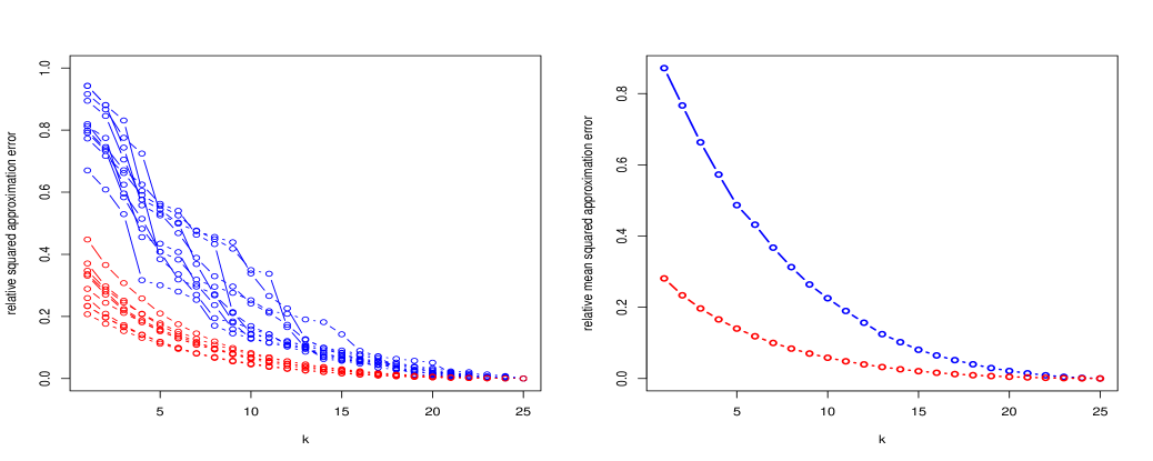
Figure 1: Relative squared low rank approximation error to $\mathbf{X}\mathcal{B}$ based on our decomposition (red) and the SVD (blue) of $\mathcal{B}$. The x-axis is the rank of the approximation matrix.

We visually illustrate the difference in approximating $\mathbf{X}\mathcal{B}$ using the two decompositions of the coefficient matrix: SVD of $\mathcal{B}$ given by $\eqref{svd.eq}$ and our decomposition given by $\eqref{70002}$ based on the SVD of $\mathbf{X}\mathcal{B}$, in Figure 1 through an example. We take $n=100$, $p=1000$ and $q=100$. Each row of $\mathbf{X}$ is generated from a $p$-dimensional multivariate normal distribution with mean zero. Its covariance matrix has all the diagonal elements equal to 1 and all the off-diagonal elements equal to 0.7. We generate $\mathcal{B}$ using $\mathcal{B}=\mathbf{CD}$, where $\mathbf{C}$ is $p\times 25$ and $\mathbf{D}$ is $25\times q$. Elements in the first 40 rows of $\mathbf{C}$ are independently generated from $N(0,1)$, and the other $p-40$ rows of $\mathbf{C}$ are zeros. Elements in $\mathbf{D}$ are independently generated from the uniform distribution between $-1$ and $1$. Therefore, in this example, the rank of $\mathcal{B}$ is $K=25$. We perform the simulation 100 times. In each repeat, for each $1\leq k\leq K$, we calculate the relative squared approximation error to $\mathbf{X}\mathcal{B}$ defined by $\|\mathbf{X}\mathcal{B}-\mathbf{X}\mathcal{B}_{k}\|_{F}^{2}/\|\mathbf{X}\mathcal{B}\|_{F}^{2}$, where $\mathcal{B}_{k}$ is the rank $k$ approximation matrix to $\mathcal{B}$ using our decomposition (red in Figure 1) or the SVD (blue). In Figure 1, we plot the relative error for 10 repeats in the left panel, and plot the mean relative error over 100 repeats in the right panel, when $k$ changes from 1 to $K=25$.

In the following, for any $1\leq k\leq K$, let $\mathcal{B}_{k}=\boldsymbol{\alpha}_{1}\mathbf{w}_{1}^{\rm T}+\cdots+\boldsymbol{\alpha}_{k}\mathbf{w}_{k}^{\rm T}$, the sum of the first $k$ terms of our decomposition. We will show in Section 3.2 that the property that $\mathbf{X}\mathcal{B}_{k}$ is the best rank $k$ approximation to $\mathbf{X}\mathcal{B}$ leads to the property that $\mathcal{B}_{k}$ has nearly the smallest expected prediction errors among all possible rank $k$ approximation to $\mathcal{B}$ under the row-wise sparsity assumption on $\mathcal{B}$. Our decomposition of $\mathcal{B}$ leads to the following model transformation,

$$\mathbf{Y}=\mathbf{X}\mathcal{B}+\boldsymbol{\varepsilon}=\mathbf{T}\mathbf{W}^{\rm T}+\boldsymbol{\varepsilon}=\mathbf{t}_{1}\mathbf{w}_{1}^{\rm T}+\cdots+\mathbf{t}_{K}\mathbf{w}_{K}^{\rm T}+\boldsymbol{\varepsilon},$$ (2.8)

where

$$\mathbf{T}=[\mathbf{t}_{1},\cdots,\mathbf{t}_{K}]\;,\text{ and }\mathbf{t}_{j}=\mathbf{X}\boldsymbol{\alpha}_{j}=\sqrt{n}\boldsymbol{\gamma}_{j},\quad 1\leq j\leq K,$$ (2.9)

are new orthogonal predictors.

To estimate the decomposition, we first estimate $\boldsymbol{\alpha}_{1},\cdots,\boldsymbol{\alpha}_{K}$ based on the following theorem, then estimate $\mathbf{t}_{1},\cdots,\mathbf{t}_{K}$ by $\eqref{70019}$. Finally, based on model $\eqref{modeltw.eq}$ and the least squares method, we obtain the estimates of $\mathbf{w}_{1},\cdots,\mathbf{w}_{K}$. Define

$$\mathbf{Z}=\frac{1}{\sqrt{n}}\mathbf{X},\quad\boldsymbol{\Xi}=\frac{1}{n}(\mathbf{X}\mathcal{B})(\mathbf{X}\mathcal{B})^{\rm T}=\mathbf{Z}\mathcal{B}\mathcal{B}^{\rm T}\mathbf{Z}^{\rm T},\quad\mathbf{S}=\frac{1}{n}\mathbf{X}^{\rm T}\mathbf{X}=\mathbf{Z}^{\rm T}\mathbf{Z},$$

$$\mathbf{B}=\frac{1}{n^{2}}\mathbf{X}^{\rm T}\left(\mathbf{X}\mathcal{B}\right)\left(\mathbf{X}\mathcal{B}\right)^{\rm T}\mathbf{X}=\mathbf{S}\mathcal{B}\mathcal{B}^{\rm T}\mathbf{S}=\mathbf{Z}^{\rm T}\boldsymbol{\Xi}\mathbf{Z}.$$ (2.10)

Theorem 2.1.

Suppose that the $n\times n$ nonnegative definite matrix $\boldsymbol{\Xi}$ has $K$ positive eigenvalues $\mu_{1}(\boldsymbol{\Xi})\geq\mu_{2}(\boldsymbol{\Xi})\geq\cdots\geq\mu_{K}(\boldsymbol{\Xi})>0$. Then

• $K\leq\min\{n,p,q\}$. For any $1\leq k\leq K$, $\boldsymbol{\alpha}_{k}$ in $\eqref{70002}$ is the solution to

  $$\max_{\boldsymbol{\alpha}\in\mathbb{R}^{p}}\quad\boldsymbol{\alpha}^{\rm T}\mathbf{B}\boldsymbol{\alpha},\quad\text{\rm subject to}\quad\boldsymbol{\alpha}^{\rm T}\mathbf{S}\boldsymbol{\alpha}=1,\quad\boldsymbol{\alpha}_{l}^{\rm T}\mathbf{S}\boldsymbol{\alpha}=0,\quad 1\leq l\leq k-1.$$ (2.11)

  Moreover, the maximum value of $\eqref{2220}$ is equal to $\boldsymbol{\alpha}_{k}^{\rm T}\mathbf{B}\boldsymbol{\alpha}_{k}=\mu_{k}(\boldsymbol{\Xi})$.

• In the SVD $\eqref{70006}$ of $\mathbf{X}\mathcal{B}$, the singular values are $\sigma_{k}=\sqrt{n\mu_{k}(\boldsymbol{\Xi})}$, $1\leq k\leq K$. The left-singular vectors satisfy

  $$\boldsymbol{\gamma}_{1}=\mathbf{Z}\boldsymbol{\alpha}_{1},\quad\boldsymbol{\gamma}_{2}=\mathbf{Z}\boldsymbol{\alpha}_{2},\quad\cdots,\quad\boldsymbol{\gamma}_{K}=\mathbf{Z}\boldsymbol{\alpha}_{K},$$ (2.12)

  and they are the $K$ eigenvectors of $\boldsymbol{\Xi}$ corresponding to the $K$ positive eigenvalues with $\|\boldsymbol{\gamma}_{k}\|_{2}=1$.

• The approximation error of the best rank $k$ approximation to $\mathbf{X}\mathcal{B}$ is

  $$\|\mathbf{X}\mathcal{B}-\sum_{i=1}^{k}\mathbf{t}_{i}\mathbf{w}_{i}^{\rm T}\|_{F}^{2}=\|\mathbf{X}\mathcal{B}-\mathbf{X}(\sum_{i=1}^{k}\boldsymbol{\alpha}_{i}\mathbf{w}_{i}^{\rm T})\|_{F}^{2}=\|\mathbf{X}\mathcal{B}-\mathbf{X}\mathcal{B}_{k}\|_{F}^{2}=n\sum_{i=k+1}^{K}\mu_{i}(\boldsymbol{\Xi})$$

  for any $1\leq k\leq K$.

By Theorem 2.1(b), $\mu_{k}(\boldsymbol{\Xi})=\sigma_{k}^{2}/n=\|\sigma_{k}\boldsymbol{\gamma}_{k}\mathbf{u}_{k}^{\rm T}\|_{F}^{2}/n$. So $\mu_{k}(\boldsymbol{\Xi})$ can be viewed as a measure of the magnitude of the signal in the $k$-th component of the SVD of $\mathbf{X}\mathcal{B}$. Therefore, our choice of $\mathbf{W}$ and $\mathbf{A}$ makes the signal concentrated in the first few components as much as possible. Theorem 2.1(c) implies that, even if $K$ is not small, as long as $\mu_{k}(\boldsymbol{\Xi})$ decreases fast enough, $\mathbf{X}\mathcal{B}$ can be well approximated by the first few components. We call this the Signal Extraction multivariate Regression (SiER) method.

To estimate $\boldsymbol{\alpha}_{k}$, we estimate $\mathbf{B}$ by

$$\widehat{\mathbf{B}}=\frac{1}{n^{2}}\mathbf{X}^{\rm T}(\mathbf{Y}-\mathbf{1}_{n}\bar{\mathbf{y}}^{\rm T})(\mathbf{Y}-\mathbf{1}_{n}\bar{\mathbf{y}}^{\rm T})^{\rm T}\mathbf{X}\;,$$ (2.13)

where $\bar{\mathbf{y}}$ is the sample mean of $\mathbf{y}_{1},\cdots,\mathbf{y}_{n}$, and $\mathbf{1}_{n}$ is an $n$-dimensional vector with all elements equal to one. In the classic setting of small $p$ and large $n$, the estimates $\widehat{\boldsymbol{\alpha}}_{1}$, $\cdots$, $\widehat{\boldsymbol{\alpha}}_{K}$ can be sequentially obtained by solving

$$\max_{\boldsymbol{\alpha}\in\mathbb{R}^{p}}\quad\boldsymbol{\alpha}^{\rm T}\widehat{\mathbf{B}}\boldsymbol{\alpha},\quad\text{\rm subject to}\quad\boldsymbol{\alpha}^{\rm T}\mathbf{S}\boldsymbol{\alpha}=1,\quad\widehat{\boldsymbol{\alpha}}_{l}^{\rm T}\mathbf{S}\boldsymbol{\alpha}=0,\quad 1\leq l\leq k-1,$$ (2.14)

where $1\leq k\leq K$. Once we obtain $\widehat{\boldsymbol{\alpha}}_{k}$, we have $\widehat{\mathbf{t}}_{k}=\mathbf{X}\widehat{\boldsymbol{\alpha}}_{k}$, which has zero sample mean. With the constraints in $\eqref{10096}$, $\widehat{\mathbf{t}}_{1},\widehat{\mathbf{t}}_{2},\ldots,\widehat{\mathbf{t}}_{K}$ are orthogonal and satisfy $\|\widehat{\mathbf{t}}_{k}\|_{2}^{2}/n=1$. Let $\widehat{\mathbf{T}}=[\widehat{\mathbf{t}}_{1},\cdots,\widehat{\mathbf{t}}_{K}]$. Then $\widehat{\mathbf{T}}^{\rm T}\widehat{\mathbf{T}}=n\mathbf{I}_{K}$, where $\mathbf{I}_{K}$ is the $K$-dimensional identity matrix. The matrix $\mathbf{W}$ is estimated by regressing $\mathbf{Y}$ on $\widehat{\mathbf{t}}_{1},\widehat{\mathbf{t}}_{2},\ldots,\widehat{\mathbf{t}}_{K}$ with the usual least squares method. That is,

$$\widehat{\mathbf{W}}^{\rm T}=(\widehat{\mathbf{T}}^{\rm T}\widehat{\mathbf{T}})^{-1}\widehat{\mathbf{T}}^{\rm T}(\mathbf{Y}-\mathbf{1}_{n}\bar{\mathbf{y}}^{\rm T})=\frac{1}{n}\widehat{\mathbf{T}}^{\rm T}(\mathbf{Y}-\mathbf{1}_{n}\bar{\mathbf{y}}^{\rm T}),$$

and $$\widehat{\mathcal{B}}=\widehat{\boldsymbol{\alpha}}_{1}\widehat{\mathbf{w}}_{1}^{\rm T}+\widehat{\boldsymbol{\alpha}}_{2}\widehat{\mathbf{w}}_{2}^{\rm T}+\cdots+\widehat{\boldsymbol{\alpha}}_{k}\widehat{\mathbf{w}}_{K}^{\rm T},$$ (2.15)

is the estimate of $\mathcal{B}$, and $\widehat{\mathcal{B}}_{k}=\widehat{\boldsymbol{\alpha}}_{1}\widehat{\mathbf{w}}_{1}^{\rm T}+\widehat{\boldsymbol{\alpha}}_{2}\widehat{\mathbf{w}}_{2}^{\rm T}+\cdots+\widehat{\boldsymbol{\alpha}}_{k}\widehat{\mathbf{w}}_{k}^{\rm T}$ is the estimate of $\mathcal{B}_{k}$. Due to the orthogonality of $\widehat{\mathbf{t}}_{1},\widehat{\mathbf{t}}_{2},\ldots,\widehat{\mathbf{t}}_{K}$, $\widehat{\mathcal{B}}_{k}$ does not depend on the number of selected components in practice. The following lemma shows that in the special case of scalar response ($q=1$), our estimate $\widehat{\mathcal{B}}$ in $\eqref{10116}$ is equivalent to the least squares method. But if $q>1$, this method may not be the same as the least squares method.

Lemma 1.

Suppose that $\mathbf{S}$ is full rank. If $q=1$, the estimate in $\eqref{10116}$ is exactly the same as the least squares estimate.

We will introduce the sparse method for the high-dimensional setting in the next section.

3 Sparse estimates and oracle inequalities in high-dimensional settings

3.1 Sparse estimates

We make the following sparsity assumption: only a small number of the coefficient vectors, $\boldsymbol{\beta}_{1},\cdots,\boldsymbol{\beta}_{p}$, are nonzero vectors. Since these vectors are the row vectors of $\mathcal{B}$, this assumption is just the row-wise sparsity of $\mathcal{B}$. The definition $\eqref{70002}$ implies that $\boldsymbol{\alpha}_{k}$ is a sparse vector and the number of its nonzero coordinates is less than or equal to the number of nonzero vectors among $\boldsymbol{\beta}_{1},\cdots,\boldsymbol{\beta}_{p}$. Motivated by the sparsity of $\boldsymbol{\alpha}_{k}$, we propose the following penalized optimization problem whose solution is the sparse estimate $\widehat{\boldsymbol{\alpha}}_{k}$ of ${\boldsymbol{\alpha}}_{k}$:

$$\max_{\boldsymbol{\alpha}\in\mathbb{R}^{p}}\quad \frac{\boldsymbol{\alpha}^{\rm T}\widehat{\mathbf{B}}\boldsymbol{\alpha}}{\boldsymbol{\alpha}^{\rm T}\mathbf{S}\boldsymbol{\alpha}+\tau\|\boldsymbol{\alpha}\|^{2}_{\lambda}},$$ (3.1)

subject to $$\boldsymbol{\alpha}^{\rm T}\mathbf{S}\boldsymbol{\alpha}=1,\quad\widehat{\boldsymbol{\alpha}}_{l}^{\rm T}\mathbf{S}\boldsymbol{\alpha}=0,\quad 1\leq l\leq k-1,$$

where $\|\boldsymbol{\alpha}\|^{2}_{\lambda}=(1-\lambda)\|\boldsymbol{\alpha}\|_{2}^{2}+\lambda\|\boldsymbol{\alpha}\|_{1}^{2}$, and both $\tau\geq 0$ and $0\leq\lambda<1$ are tuning parameters. In the penalty $\tau\|\boldsymbol{\alpha}\|^{2}_{\lambda}$, the $l_{2}$ term is used to overcome the singularity problem of $\mathbf{S}$ and the $l_{1}$ term encourages the sparsity of $\widehat{\boldsymbol{\alpha}}_{k}$. The penalty $\tau\|\boldsymbol{\alpha}\|^{2}_{\lambda}$ was introduced in Qi, Luo and Zhao (2013) for sparse principal component analysis and utilized in Qi, Luo, Carroll and Zhao (2015) for sparse regression and sparse discriminant analysis. The main reason that we use the squared $l_{1}$ norm instead of the $l_{1}$ norm itself as in the elastic-net is to make the objective function in $\eqref{1240}$ scale-invariant, that is, if we replace $\boldsymbol{\alpha}$ by $t\boldsymbol{\alpha}$, where $t$ is any nonzero number, the value of the objective function is unchanged. This property plays an important role in our theoretical development and algorithms. Due to the scale-invariant property, $\eqref{1240}$ is equivalent to

$$\max{\boldsymbol{\alpha}^{\rm T}\widehat{\mathbf{B}}\boldsymbol{\alpha}}\quad\text{subject to}\quad\boldsymbol{\alpha}^{\rm T}\mathbf{S}\boldsymbol{\alpha}+\tau\|\boldsymbol{\alpha}\|^{2}_{\lambda}\leq 1\text{ and }\boldsymbol{\alpha}^{\rm T}\mathbf{S}\widehat{\boldsymbol{\alpha}}_{l}=0,\quad 1\leq l\leq k-1.$$ (3.2)

In fact, the solutions of $\eqref{1240}$ and $\eqref{alg.eq}$ differ only by a scale factor. We have proposed algorithms to solve a more general optimization problem (see the problem (4.3) in Qi et al. (2015)) than $\eqref{alg.eq}$. By a proper rescaling of the solution to $\eqref{alg.eq}$, we obtain $\widehat{\boldsymbol{\alpha}}_{k}$. With the constraints in $\eqref{1240}$, the estimates $\widehat{\mathbf{t}}_{k}=\mathbf{X}\widehat{\boldsymbol{\alpha}}_{k}$, $1\leq k\leq K$, are still orthogonal to each other and satisfy $\|\widehat{\mathbf{t}}_{k}\|_{2}^{2}/n=1$. Therefore, we can use $\eqref{10116}$ to get the estimates $\widehat{\mathbf{W}}$ and $\widehat{\mathcal{B}}$. In the special case of scalar response, the proposed method is just the sparse regression by projection method proposed in Qi et al. (2015).

3.2 Oracle inequalities

In this section, we provide oracle inequalities for the estimates of $\boldsymbol{\alpha}_{k}$, $\mathbf{w}_{k}$ and $\mathcal{B}$ in high-dimensional settings. These oracle inequalities hold for any $n$ and $p$.

We follow the notations in Bickel et al. (2009). For any $p$-dimensional vector $\mathbf{a}=(a_{1},\cdots,a_{p})^{\rm T}$, let $J(\mathbf{a})=\{j\in\{1,\cdots,p\}:a_{j}\neq 0\}$ denote the collection of indices of nonzero coordinates of $\mathbf{a}$ and $\mathcal{M}(\mathbf{a})=|J(\mathbf{a})|$ denote the number of nonzero coordinates of $\mathbf{a}$, where $|J(\mathbf{a})|$ is the cardinality of $J(\mathbf{a})$. $\mathcal{M}(\mathbf{a})$ is a measure of the sparsity of $\mathbf{a}$. Similarly, for any $p\times q$ matrix $\widetilde{\mathcal{B}}$ with row vectors, $\widetilde{\boldsymbol{\beta}}_{1}$, $\cdots$, $\widetilde{\boldsymbol{\beta}}_{p}$, we define $J(\widetilde{\mathcal{B}})=\{j\in\{1,\cdots,p\}:\widetilde{\boldsymbol{\beta}}_{j}\neq\mathbf{0}\}$ and $\mathcal{M}(\widetilde{\mathcal{B}})=|J(\widetilde{\mathcal{B}})|$ which is a measure of the row-wise sparsity of $\widetilde{\mathcal{B}}$. It follows from $\eqref{70002}$ that

$$J(\boldsymbol{\alpha}_{k})\subset J(\mathcal{B}),\quad\text{ and hence}\quad\mathcal{M}(\boldsymbol{\alpha}_{k})\leq\mathcal{M}(\mathcal{B}),\quad\forall 1\leq k\leq K.$$ (3.3)

Before we provide the main results, we first show that $\mathcal{B}_{k}$ has nearly the smallest expected prediction error among all rank $k$ coefficient matrix estimations when $n$ is large. Let $\mathbf{x}^{\rm new}$ be a new observation of the predictor vector and $\boldsymbol{\Sigma}$ the covariance matrix of $\mathbf{x}^{\rm new}$. The corresponding new response is $(\mathbf{y}^{\rm new})^{\rm T}=(\mathbf{x}^{\rm new})^{\rm T}\mathcal{B}+(\boldsymbol{\varepsilon}^{\rm new})^{\rm T}$, where $\boldsymbol{\varepsilon}^{\rm new}$ is independent of $\mathbf{x}^{\rm new}$.

Theorem 3.1.

Suppose that $\|\mathbf{S}-\boldsymbol{\Sigma}\|_{\infty}\leq C\sqrt{\frac{\log p}{n}}$, where $C$ is a constant which does not depend on $n$ and $p$. Then we have

$$E\left[\|(\mathbf{x}^{\rm new})^{\rm T}\mathcal{B}_{k}-(\mathbf{y}^{\rm new})^{\rm T}\|_{2}^{2}\right]\leq\min_{\widetilde{\mathcal{B}_{k}}}E\left[\|(\mathbf{x}^{\rm new})^{\rm T}\widetilde{\mathcal{B}}_{k}-(\mathbf{y}^{\rm new})^{\rm T}\|_{2}^{2}\right]+2C\|\mathcal{B}\|_{F}^{2}\mathcal{M}(\mathcal{B})\sqrt{\frac{\log p}{n}},$$

where the minimum is taken over all possible $\widetilde{\mathcal{B}}_{k}$ of the forms $\sum_{j=1}^{k}\mathbf{b}_{j}\mathbf{v}_{j}^{\rm T}$ with arbitrary $\mathbf{b}_{j}\in\mathbb{R}^{p}$ and $\mathbf{v}_{j}\in\mathbb{R}^{q}$.

Note that when $q=1$, $\mathcal{M}(\mathcal{B})\sqrt{\log p/n}$ is the convergence rate of the LASSO and the Dantzig selector (Bickel et al., 2009). Under the sparsity assumption that when $n$, $p\to\infty$, $\|\mathcal{B}\|_{F}^{2}\mathcal{M}(\mathcal{B})\sqrt{\log{p}/n}\to 0$, the expected prediction error of $\mathcal{B}_{k}$ is close to the smallest one among all possible rank $k$ approximation to $\mathcal{B}$ when $n$ and $p$ are large. We assume that $\|\mathbf{S}-\boldsymbol{\Sigma}\|_{\infty}\leq C\sqrt{\log{p}/n}$, because it has been shown (Equation (A14) in Bickel and Levina (2008)) that $\sqrt{\log{p}/n}$ is the order of the max norm of the difference between the sample covariance matrix and the population covariance matrix of $p$-dimensional multivariate normal distribution.

Now we state three regularity conditions for the main theorems. In the setting of large $p$ and small $n$, the identification problem exists for the model $\eqref{100003}$. That is, there exists $\widetilde{\mathcal{B}}\neq\mathcal{B}$ such that $\mathbf{X}\widetilde{\mathcal{B}}=\mathbf{X}\mathcal{B}$. Bickel et al. (2009) imposed the following restricted eigenvalue assumptions on $\mathbf{X}$, which we will also adopt here.

Condition 1.

Let $s=\mathcal{M}(\mathcal{B})$ and

$$\kappa=\min_{\begin{subarray}{c}J_{0}\subset\{1,\cdots,p\},\\ |J_{0}|\leq s\end{subarray}}\min_{\begin{subarray}{c}\mathbf{0}\neq\boldsymbol{\delta}\in\mathbf{R}^{p},\\ \left\|\boldsymbol{\delta}_{J_{0}^{c}}\right\|_{1}\leq c\left\|\boldsymbol{\delta}_{J_{0}}\right\|_{1}\end{subarray}}\frac{\|\mathbf{X}\boldsymbol{\delta}\|_{2}}{\sqrt{n}\|\boldsymbol{\delta}_{J_{0}}\|_{2}},$$

where $c>1$ and $\kappa>0$ are two constants, $\boldsymbol{\delta}_{J_{0}}$ and $\boldsymbol{\delta}_{J_{0}^{c}}$ are the subvectors of $\boldsymbol{\delta}$ consisted of the coordinates with indices belonging to $J_{0}$ and $J_{0}^{c}$, respectively.

A consequence of this restricted eigenvalue assumption is that for any two $p$-dimensional vectors, $\boldsymbol{\alpha}$ and $\boldsymbol{\alpha}^{\prime}$ with sparsity $\mathcal{M}(\boldsymbol{\alpha})\leq s$ and $\mathcal{M}(\boldsymbol{\alpha}^{\prime})\leq s$, if $\mathbf{X}\boldsymbol{\alpha}=\mathbf{X}\boldsymbol{\alpha}^{\prime}$, then we have $\boldsymbol{\alpha}=\boldsymbol{\alpha}^{\prime}$ (see the second remark after Theorem 7.3 in Bickel et al. (2009)). Therefore, the model $\eqref{100003}$ is identifiable among all coefficient matrices with row-wise sparsity less than or equal to $\mathcal{M}(\mathcal{B})$. Therefore, if $\mathbf{X}\mathcal{B}^{\prime}=\mathbf{X}\mathcal{B}$ and $\mathcal{M}(\mathcal{B}^{\prime})\leq s=\mathcal{M}(\mathcal{B})$, then $\mathcal{B}^{\prime}=\mathcal{B}$.

The next regularity condition is on the distribution of the $q$-dimensional noise vector $\boldsymbol{\varepsilon}_{i}$.

Condition 2.

The random error vectors $\boldsymbol{\varepsilon}_{i}$, $1\leq i\leq n$, are i.i.d. mean zero $\mathbb{R}^{q}$-valued Gaussian variables with median $M_{\varepsilon}$ and variance $\sigma^{2}$, where $M_{\varepsilon}$ is defined as the median of the real-valued random variable $\|\boldsymbol{\varepsilon}_{i}\|_{2}$ and the variance is defined as $\sigma^{2}=\sup_{\mathbf{u}\in\mathbb{R}^{q},\|\mathbf{u}\|_{2}=1}E[(\mathbf{u}^{\rm T}\boldsymbol{\varepsilon}_{i})^{2}]$ (Section 3.1 in Ledoux and Talagrand (2011)).

Note that $(\mathbf{u}^{\rm T}\boldsymbol{\varepsilon}_{i})$ is the projection of $\boldsymbol{\varepsilon}_{i}$ onto the direction of $\mathbf{u}$, and has a normal distribution. Hence, $\sigma^{2}$ is the maximum of the variances of the projections of $\boldsymbol{\varepsilon}_{i}$ along all possible directions in $\mathbb{R}^{q}$. In the special case $q=1$, $\sigma^{2}$ is the just usual variance. In our theoretical development, we need to estimate the tail probabilities of $\|\boldsymbol{\varepsilon}_{i}\|_{2}$ which can be controlled by $M_{\varepsilon}$ and $\sigma^{2}$ (Section 3.1 in Ledoux and Talagrand (2011)). Bunea et al. (2012) assumes that the coordinates $\{\varepsilon_{ij}:1\leq j\leq q\}$ of $\boldsymbol{\varepsilon}_{i}$ have independent and identical normal distributions. Condition 2 is weaker and allows correlations among ${\varepsilon}_{i1},\ldots,{\varepsilon}_{iq}$.

Condition 3.

All the diagonal elements of $\mathbf{S}=\mathbf{X}^{\rm T}\mathbf{X}/n$ are equal to 1 and there exist positive constants, $c_{2}$ and $c_{3}$, such that

• $\min\left\{\frac{\mu_{1}(\boldsymbol{\Xi})-\mu_{2}(\boldsymbol{\Xi})}{\mu_{1}(\boldsymbol{\Xi})},\quad\frac{\mu_{2}(\boldsymbol{\Xi})-\lambda_{3}(\boldsymbol{\Xi})}{\mu_{2}(\boldsymbol{\Xi})},\cdots,\frac{\mu_{K-1}(\boldsymbol{\Xi})-\mu_{K}(\boldsymbol{\Xi})}{\mu_{K-1}(\boldsymbol{\Xi})}\right\}\geq c_{2}$,

• $\mu_{1}(\boldsymbol{\Xi})/\mu_{K}(\boldsymbol{\Xi})\leq c_{3}$.

Bickel et al. (2009) assumed that the diagonal elements of $\mathbf{S}=\mathbf{X}^{\rm T}\mathbf{X}/n$ are equal to 1, which can be achieved by scaling $\mathbf{X}$. Condition 3 (a) prevents the cases where the spacing between adjacent eigenvalues is so small that the eigenvalues cannot be well separated based on noisy observations. Condition 3 (b) excludes the situations where the magnitudes of the higher order components are too small compared to those of lower order components.

As mentioned in Section 2, in the classic setting, if $q>1$, our method $\eqref{10009}$ may not be the same as the least squares method. For the integrity of this paper, below we first provide the asymptotic result for our method in Theorem 3.2 under the setting when $p$ is fixed and $n$ goes to infinity, and then provide the theoretical property of our sparse estimates for high dimensional setting afterward.

Theorem 3.2.

Suppose that Conditions 2-3 hold with $M_{\varepsilon}$, $\sigma^{2}$ and $c_{3}$ bounded above and $c_{2}$ bounded below as $n\to\infty$. Moreover, we assume that there exists $c_{0}>0$ independent of $n$ such that $\mathbf{S}$ is positive definite and its smallest eigenvalue, $\lambda_{min}(\mathbf{S})\geq c_{0}$, for all $n$ large enough. Then we have

$$\|\widehat{\mathcal{B}}-\mathcal{B}\|_{F}=O_{p}(1/\sqrt{n}),\quad\|\widehat{\boldsymbol{\alpha}}_{k}-\boldsymbol{\alpha}_{k}\|_{2}=\mu_{1}(\boldsymbol{\Xi})^{-1/2}O_{p}(1/\sqrt{n}),$$ (3.4)

for any $1\leq k\leq K$.

In the rest of this section, we study the theoretical property of our sparse estimates $\widehat{\boldsymbol{\alpha}}_{k}$ and $\widehat{\mathcal{B}}$ when both $n,p\to\infty$. We first provide upper bounds on the $l_{1}$ sparsity of $\widehat{\boldsymbol{\alpha}}_{k}$, $1\leq k\leq K$, and the oracle inequalities for them in the following theorem. Although we use the same tuning parameters $(\tau,\lambda)$ in $\eqref{1240}$ for all components in practice for the computational efficiency, in our theoretical results, we allow different tuning parameters for different components. We use $(\tau^{(k)},\lambda^{(k)})$ to denote the tuning parameters for the $k$-th component, $1\leq k\leq K$. Let $\widehat{\boldsymbol{\gamma}}_{k}=\mathbf{Z}\widehat{\boldsymbol{\alpha}}_{k}=\widehat{\mathbf{t}}_{k}/\sqrt{n}$, $1\leq k\leq K$, which are estimates of $\boldsymbol{\gamma}_{k}=\mathbf{Z}\boldsymbol{\alpha}_{k}=\mathbf{t}_{k}/\sqrt{n}$. Define

$$\varpi=\sqrt{\frac{\log{p}}{n}},\quad\text{\rm and recall that }\quad s=\mathcal{M}(\mathcal{B}).$$

Theorem 3.3.

Assume that Conditions 1-3 hold. Suppose that

$$\mu_{1}(\boldsymbol{\Xi})\geq\hbar^{2}C_{0}^{2}\varpi^{2}s/\kappa^{2},\quad\text{where }C_{0}=2\max\{M_{\varepsilon}/\sqrt{\log{2}},2\sigma\},$$ (3.5)

$\kappa$ is the constant in Condition 1 and $\hbar$ is a constant. Let the tuning parameters $(\tau^{(k)},\lambda^{(k)})$, $1\leq k\leq K$, satisfy conditions

$$\tau^{(k)}=\frac{A^{(k)}C_{0}\varpi}{\|\boldsymbol{\alpha}_{1}\|_{1}\sqrt{\mu_{1}(\boldsymbol{\Xi})}},\qquad c^{-1}+\delta_{0}<\lambda^{(k)}\leq 1,$$ (3.6)

where $A^{(k)}$ and $\delta_{0}$ are positive constants such that $c^{-1}+\delta_{0}<1$, and $c$ is the constant in Condition 1.

• For the first component ($k=1$), there exist constants $A_{1}^{L}$ and $\hbar_{0}$ which only depend on $c$, $c_{2}$ and $\delta_{0}$, where $c_{2}$ is the constant in Condition 3 (a), such that with probability at least $1-2e^{M_{\varepsilon}^{2}/2\sigma^{2}}p^{1-C_{0}^{2}/4\sigma^{2}}$, if $A^{(1)}\geq A_{1}^{L}$ and $\hbar\geq\hbar_{0}$, we have

  $$\|\widehat{\boldsymbol{\alpha}}_{1}\|_{1}\leq\sqrt{6c}\|\boldsymbol{\alpha}_{1}\|_{1}\leq\sqrt{6cs}/\kappa,$$ (3.7)

  $$\|\widehat{\boldsymbol{\alpha}}_{1}-\boldsymbol{\alpha}_{1}\|_{1}\leq 4(1+c)(1+\sqrt{6c})c_{2}^{-1}A^{(1)}C_{0}\kappa^{-2}\mu_{1}(\boldsymbol{\Xi})^{-1/2}\varpi s,$$

  $$\frac{1}{n}\|\mathbf{X}(\widehat{\boldsymbol{\alpha}}_{1}-\boldsymbol{\alpha}_{1})\|_{2}^{2}=\|\widehat{\boldsymbol{\gamma}}_{1}-\boldsymbol{\gamma}_{1}\|_{2}^{2}\leq 16c_{2}^{-2}(1+\sqrt{6c})^{2}(A^{(1)}C_{0}/\kappa)^{2}\mu_{1}(\boldsymbol{\Xi})^{-1}\varpi^{2}s.$$

• For the higher order components ($1<k\leq K$), we further assume that

  $$\max_{1\leq k\leq K}\|\boldsymbol{\alpha}_{k}\|_{1}\leq c_{4}\min_{1\leq k\leq K}\|\boldsymbol{\alpha}_{k}\|_{1},\quad\kappa^{-2}\mu_{1}(\boldsymbol{\Xi})^{-1/2}C_{0}\varpi s\leq c_{5}\|\boldsymbol{\alpha}_{1}\|_{1},$$ (3.8)

  where $c_{4}$ and $c_{5}$ are two constants. Then there exist constants $\hbar_{0}$, $A^{L}_{j}<A^{U}_{j}$, $1\leq j\leq K$, which only depend on $\delta_{0}$, $c$, $c_{2}\sim c_{5}$, such that with probability at least $1-2e^{M_{\varepsilon}^{2}/2\sigma^{2}}p^{1-C_{0}^{2}/4\sigma^{2}}$, for any $1\leq k\leq K$, if $A^{L}_{j}\leq A^{(j)}\leq A^{U}_{j}$, $1\leq j<k$, $A^{(k)}\geq A^{L}_{k}$ and $\hbar\geq\hbar_{0}$, we have

  $$\|\widehat{\boldsymbol{\alpha}}_{k}\|_{1}\leq D_{k,1}\sqrt{s}/\kappa,\quad\|\widehat{\boldsymbol{\alpha}}_{k}-\boldsymbol{\alpha}_{k}\|_{1}\leq D_{k,4}A^{(k)}C_{0}\kappa^{-2}\mu_{1}(\boldsymbol{\Xi})^{-1/2}\varpi s,,$$ (3.9)

  $$\frac{1}{n}\|\mathbf{X}(\widehat{\boldsymbol{\alpha}}_{k}-\boldsymbol{\alpha}_{k})\|_{2}^{2}=\|\widehat{\boldsymbol{\gamma}}_{k}-\boldsymbol{\gamma}_{k}\|^{2}_{2}\leq D_{k,2}(A^{(k)}C_{0}/\kappa)^{2}\mu_{1}(\boldsymbol{\Xi})^{-1}\varpi^{2}s\;,$$

  where $D_{k,1}$, $D_{k,2}$ and $D_{k,4}$ are constants only depending on $\delta_{0}$, $c$, $c_{2}\sim c_{5}$.

In the upper bounds above, only $C_{0}$ depends on the distribution of the noise vector $\boldsymbol{\varepsilon}_{i}$ and can be regarded as a measure of the magnitude of noise. Although we have two tuning parameters, $\tau^{(k)}$ and $\mu^{(k)}$, for each $k$, by Theorem 3.3, $\lambda^{(k)}$ is not essential for the convergence rates. Actually, it can be any number in a subinterval of the interval $(c^{-1},1]$ and does not affect the convergence rates. However, the choice of $\lambda^{(k)}$ does affect the predictive performance in the finite-sampling situations. We will propose methods to choose these two parameters in the following section. Now we provide the oracle inequalities for $\widehat{\mathbf{W}}$, $\widehat{\mathcal{B}}$ and $\mathbf{X}\widehat{\mathcal{B}}$. We will consider the case $q=1$ first and then $q>1$. When $q=1$, we use $\boldsymbol{\beta}$ to denote the coefficient vector $\mathcal{B}$ and $\mathbf{W}=\mathbf{w}_{1}$ is a scalar.

Theorem 3.4.

Let $q=1$ and $\boldsymbol{\varepsilon}_{i}\sim N(0,\sigma^{2})$. Suppose that Condition 1 holds and $\|\mathbf{X}\boldsymbol{\beta}\|_{2}^{2}/n\geq\hbar^{2}\sigma^{2}\varpi^{2}s/\kappa^{2}$, where $\kappa$ is the constant in Condition 1. Let the tuning parameters $(\tau,\lambda)$ satisfy

$$\tau=\frac{A\sigma\varpi}{\|\boldsymbol{\alpha}_{1}\|_{1}\|\mathbf{X}\boldsymbol{\beta}\|_{2}/\sqrt{n}},\qquad c^{-1}+\delta_{0}<\lambda\leq 1,$$

where $A$ is a constant large enough and $\delta_{0}$ is a constant satisfying $c^{-1}+\delta_{0}<1$. Then with probability at least $1-2\sqrt{e}p^{-3}$, we have

$$|\widehat{\mathbf{w}}_{1}-\mathbf{w}_{1}|\leq D_{1}\sigma\kappa^{-1}\varpi\sqrt{s},\quad\|\widehat{\boldsymbol{\beta}}-\boldsymbol{\beta}\|_{1}\leq D_{3}\sigma\kappa^{-2}\varpi s,\quad\|\mathbf{X}(\widehat{\boldsymbol{\beta}}-\boldsymbol{\beta})\|_{2}\leq\sqrt{n}D_{4}\sigma\kappa^{-1}\varpi\sqrt{s},$$

where $D_{1}$, $D_{3}$ and $D_{4}$ are constants only depending on $A$, $c$, $\hbar$ and $c_{2}$.

The upper bounds of $\|\widehat{\boldsymbol{\beta}}-\boldsymbol{\beta}\|_{1}$ and $\|\mathbf{X}(\widehat{\boldsymbol{\beta}}-\boldsymbol{\beta})\|_{2}$ in Theorem 3.4 are the same as those for the Lasso and the Dantzig selector (Bickel et al., 2009) except the constants.

When $q>1$, to measure the difference between $\widehat{\mathcal{B}}$ and $\mathcal{B}$, we consider the $L_{1,2}$ norm which is defined by

$$\|\mathbf{M}\|_{1,2}=\left[\sum_{j=1}^{m}\left(\sum_{i=1}^{l}|M_{ij}|\right)^{2}\right]^{1/2},$$

where $\mathbf{M}$ is any $l\times m$ matrix and $M_{ij}$ is the $(i,j)$ element. Then for any matrix $\mathbf{M}$, we have $\|\mathbf{M}\|_{1,2}\geq\|\mathbf{M}\|_{F}$. Therefore, convergence under the $L_{1,2}$ norm is stronger than that under the Frobenius norm. If $m=1$, $L_{1,2}$ norm is just the $l_{1}$ norm for a vector.

Theorem 3.5.

Suppose that all the conditions in Theorem 3.3 hold. Then with probability at least $1-2e^{M_{\varepsilon}^{2}/2\sigma^{2}}p^{1-C_{0}^{2}/4\sigma^{2}}$, for any $1\leq K_{0}\leq K$, if $A_{k}^{L}\leq A^{(k)}\leq A_{k}^{U}$, $1\leq k<K_{0}$, and $A^{(K_{0})}\geq A_{K_{0}}^{L}$, we have

$$\|\widehat{\mathbf{w}}_{k}-\mathbf{w}_{k}\|_{2}\leq L_{k,1}C_{0}\varpi\sqrt{s}/\kappa,\quad\|\widehat{\mathcal{B}}_{k}-\mathcal{B}_{k}\|_{1,2}\leq L_{K_{0},3}C_{0}\varpi s/\kappa^{2},$$

$$\|\mathbf{X}\widehat{\mathcal{B}}_{k}-\mathbf{X}\mathcal{B}_{k}\|_{F}\leq\sqrt{n}L_{K_{0},4}C_{0}\varpi\sqrt{s}/\kappa\;,$$

for $1\leq k\leq K_{0}$, where $L_{k,1}$, $L_{k,3}$ and $L_{k,4}$ are constants only depending on $A^{(j)}$ for $1\leq j\leq k$, $c$, $\hbar$ and $c_{2}\sim c_{5}$. In particular, when $K_{0}=K$, we have

$$\|\widehat{\mathcal{B}}-\mathcal{B}\|_{1,2}\leq L_{K,3}C_{0}\varpi s/\kappa^{2},\quad\|\mathbf{X}(\widehat{\mathcal{B}}-\mathcal{B})\|_{F}\leq\sqrt{n}L_{K,4}C_{0}\varpi\sqrt{s}/\kappa.$$

Bunea et al. (2012) provides an upper bound on $E[\|\mathbf{X}(\widehat{\mathcal{B}}-\mathcal{B})\|^{2}_{F}/n]$, which is $\{qK/n+Ks\varpi^{2}\}$ multiplied by a constant (they use different notations). This upper bound depends on $q$, the dimension of $\mathbf{Y}$, and only if $q/n\to 0$, the upper bound converges to zero. Our bound holds for arbitrary $q$, even if $q$ goes to infinity faster than $n$ and $p$.

For any $1\leq k\leq K$, $\widehat{\mathcal{B}}_{k}$ and $\mathbf{X}\widehat{\mathcal{B}}_{k}$ are estimates of $\mathcal{B}_{k}$ and $\mathbf{X}\mathcal{B}_{k}$, respectively. Theorem 3.5 and Theorem 2.1(c) imply that, even if $K$ is not small, as long as $\mu_{k}(\boldsymbol{\Xi})$ decreases fast enough, $\mathbf{X}\mathcal{B}$ can be well approximated $\mathbf{X}\widehat{\mathcal{B}}_{k}$ with a relatively small $k$.

4 Choice of the number of components and tuning parameters

In this section, we propose a method to choose the tuning parameters and decide the number of components. We first provide the rationale behind the selection method and then provide the details of the method in Algorithm 4.1. In practice, to improve computational efficiency, we use the same tuning parameters for all components and denote them as $(\tau,\lambda)$. The theoretical results in previous section imply that $\lambda$ is not essential for the convergence rates. However, it has effects on the prediction errors in the finite sample situations. With the penalty $\tau\|\boldsymbol{\alpha}\|^{2}_{\lambda}=\tau(1-\lambda)\|\boldsymbol{\alpha}\|_{2}^{2}+\tau\lambda\|\boldsymbol{\alpha}\|_{1}^{2}$, the coefficient of the squared $l_{1}$ term is $\tau\lambda$. Roughly speaking, the effect of $(\tau,\lambda)$ on the sparsity of solutions mainly depends on $\tau\lambda$ and thus a small $\tau$ with a large $\lambda$ has a similar effect on the sparsity of solutions as that of a large $\tau$ with a small $\lambda$. Hence, to improve the computational efficiency, we do not consider all the pairs of $(\tau,\lambda)$ in a two dimensional grid. Instead, we will select the parameters from a sequence of pairs where with the increase of $\tau$, $\lambda$ also increases. Specifically, in the following simulation studies and applications, we choose $(\tau,\lambda)$ from the following paired values: $(0.05,0.05)$, $(0.1,0.05)$, $(0.1,0.1)$, $(0.5,0.1)$, $(0.5,0.2)$, $(1,0.2)$, $(1,0.3)$, $(5,0.3)$, $(5,0.4)$, $(10,0.4)$, $(50,0.5)$, and $(100,0.6)$.

For each of the 12 pairs of tuning parameters, we first determine $\widehat{K}_{i}$, $1\leq i\leq 12$, the maximum number of components to be found. As $\mu_{k}(\boldsymbol{\Xi})=\boldsymbol{\alpha}_{k}^{\rm T}\mathbf{B}\boldsymbol{\alpha}_{k}$ measures the signal magnitude of the $k$-th component and $\widehat{\mu}_{k}(\boldsymbol{\Xi})=\widehat{\boldsymbol{\alpha}}_{k}^{\rm T}\widehat{\mathbf{B}}\widehat{\boldsymbol{\alpha}}_{k}$ is an estimate of $\mu_{k}(\boldsymbol{\Xi})$, we only compute the first few components with large values of $\widehat{\mu}_{k}(\boldsymbol{\Xi})$ and stop when $\widehat{\mu}_{k}(\boldsymbol{\Xi})$ becomes small enough. On the other hand, by Theorem 2.1 (a), the number of components cannot exceed $\hbox{min}(n,p,q)$. Based on these two considerations, we define

$$\widehat{K}_{i}=\min\{\widehat{K}_{i}^{(1)},\widehat{K}_{i}^{(2)}\},\quad\text{ where }\widehat{K}_{i}^{(1)}=\hbox{min}(n,p,q),$$ (4.1)

$$\text{and }\widehat{K}_{i}^{(2)}=\min\left\{k>1:\frac{\widehat{\mu}_{k}(\boldsymbol{\Xi})}{\widehat{\mu}_{1}(\boldsymbol{\Xi})+\cdots+\widehat{\mu}_{k}(\boldsymbol{\Xi})}\leq 0.05\right\}\;.$$

The $\widehat{K}_{i}^{(2)}$ implies that we stop searching for higher order components if the signal magnitude of the $k$th component does not account for more than $5\%$ (by default) of the first $k$ components. Once we have determined all the $\widehat{K}_{i}$, we use the cross-validation method to determine the tuning parameters and the optimal number of components, $\widehat{K}_{opt}$. More specifically, we summarize the procedure in the following algorithm.

Algorithm 4.1.

1. For the $i$-th paired value of the tuning parameters, $1\leq i\leq 12$, we determine $\widehat{K}_{i}$ using $\eqref{30000}$ and the whole data set.

2. Use the five-fold cross-validation to determine the number of components and the tuning parameters. We split the whole data set into five subsets and repeat the following procedure. For $1\leq l\leq 5$, we use the $l$-th subset as the $l$-th validation set and all other observations as the $l$-th training set. Then for the $i$-th pair of tuning parameter values, based on the $l$-th training set,

   1. we estimate the first $\widehat{K}_{i}$ components ($\widehat{\boldsymbol{\alpha}}_{1},\ldots,\widehat{\boldsymbol{\alpha}}_{\widehat{K}_{i}}$) by sequentially solving $\eqref{1240}$.

   2. For each $j=1,\cdots,\widehat{K}_{i}$, we define $\widehat{\mathbf{t}}_{j}=\mathbf{X}\widehat{\boldsymbol{\alpha}}_{j}$ as the $j$-th new predictor. We use the first $j$ new predictors and $\eqref{10116}$ to get the estimate $\widehat{\mathcal{B}}_{ij}^{(l)}$ of the coefficient matrix, which is the estimate based on the $l$-th training data set, the $i$-th pair of tuning parameter values and the first $j$ components.

   3. Then we apply $\widehat{\mathcal{B}}_{ij}^{(l)}$ to the $l$-th validation data set to get the validation error, $e^{(l)}_{ij}$.

   4. Finally, we calculate the average validation error, $\bar{e}_{ij}=(e^{(1)}_{ij}+\cdots+e^{(5)}_{ij})/5$, for the $i$-th pair of tuning parameter values and the first $j$ components ($j=1,\cdots,\widehat{K}_{i}$).

   Let $\bar{e}_{i_{0}j_{0}}=\min_{i,j}\bar{e}_{ij}$. Then the $i_{0}$-th paired value of tuning parameters is chosen, and the optimal number of components is $\widehat{K}_{opt}=j_{0}$.

5 Simulation studies

In this section, we compare the performance of the proposed SiER method with four related methods on simulated data. The first method is the SRRR (Chen and Huang, 2012) which assumes the reduced rank structure and estimates the lower rank decomposition of the coefficient matrix by solving a penalized least squares problem with a group-Lasso type penalty on the first lower rank matrix. The second method is RemMap (Peng et al., 2010) which does not assume the reduced rank structure and solves a penalized least squares problem with both row-wise and element-wise sparsity imposed on the coefficient matrix. The third method is the SPLS (Chun and Keles, 2010) which identifies sparse latent components by maximizing the covariance between them and the responses with sparsity penalty imposed. The last method is SepLasso which fits separate regression models using Lasso for each individual response.

We consider three cases. In each case, we will consider the effects of different factors including the dimension of the responses ($q$), the number of predictors ($p$) and their correlations ($\rho$), and the magnitude ($\sigma^{2}$) and correlation ($r$) of noises. In the first case, $q$ is small. In the last two cases, $q$ is relatively large and we generate the coefficient matrices as the product of two lower rank matrices. For each setting, we repeat the following procedure 50 times. In each replicate, we simulate 590 independent observations among which 90 are the training data and 500 are the test data. Then we apply each of the five methods to the training data to select the tuning parameters and the number of components, and construct the final model which is applied to the test data to obtain the test errors. The test error is defined as $\|\mathbf{Y}_{test}-\mathbf{Y}_{pred}\|^{2}_{F}/500$, where $\mathbf{Y}_{test}$ is the $500\times q$ matrix of the test data and $\mathbf{Y}_{pred}$ is the corresponding predicted matrix. The mean squared prediction error (MSPE) is obtained by averaging the 50 test errors.

5.1 Case 1

We generate data using the model $\mathbf{Y}=\mathbf{X}\mathcal{B}+\boldsymbol{\varepsilon}$. We fix $p=500$, $q=3$, and set $\mathcal{B}_{j1}=1/\sqrt{15}$ for $j=1,\ldots,15$, $\mathcal{B}_{j2}=0.5/\sqrt{30}$ for $j=16,\ldots,45$, $\mathcal{B}_{j3}=0.25/\sqrt{60}$ for $j=46,\ldots,105$, and $\mathcal{B}_{jk}=0$ for others. For each $i=1,\ldots,n$, the first 150 predictors are generated from multivariate normal distribution $({X}_{i1},\ldots,{X}_{i,150})^{\rm T}\sim N_{150}(0,\Sigma)$, where $\Sigma$ has the $(i,j)$-th element $\Sigma_{jk}=\rho^{|j-k|}$ for $j,k=1,\ldots,150$, and the other predictors are independent normal variables, ${X}_{ij}\sim N(0,0.1^{2})$ for $j=151,\ldots,p$. The noise vector $\boldsymbol{\varepsilon}_{i}$ is generated from $N_{q}(0,\sigma^{2}R)$, where the correlation matrix $R$ has diagonal elements 1 and off-diagonal elements $r$. In this and the following cases, we will use $q\sigma^{2}$, the sum of the diagonal elements of the covariance matrix of the noise vector $\boldsymbol{\varepsilon}_{i}$, as a measure of the noise level. We choose $\rho=0.3$ and 0.7, $q\sigma^{2}=0.1$ and 0.15, $r=0.2$ and 0.9, and consider all their possible combinations.

We draw the boxplots of MSPE in Figure 2 and show the average and standard deviation of MSPEs of 50 repeats in Table 1. The SiER has best predictive performance. In this case, $q$ is small, and there is no factor structure and no obvious group sparsity structure, so it is understandable that the SRRR has larger prediction errors than RemMap since the latter takes advantages of both the row-wise and element-wise sparsity. The SPLS has the largest MSPE because it does not directly target on prediction of the responses and thus has disadvantage in terms of prediction. The correlation among predictors, $\rho$, has a large effect on MSPE for all methods. A stronger correlation leads to a smaller prediction error in all the methods. The correlation in random error, $r$, does not have obvious effects on MSPE for all methods. Increasing in the magnitude of random error ($q\sigma^{2}$) unsurprisingly leads to higher MSPE.

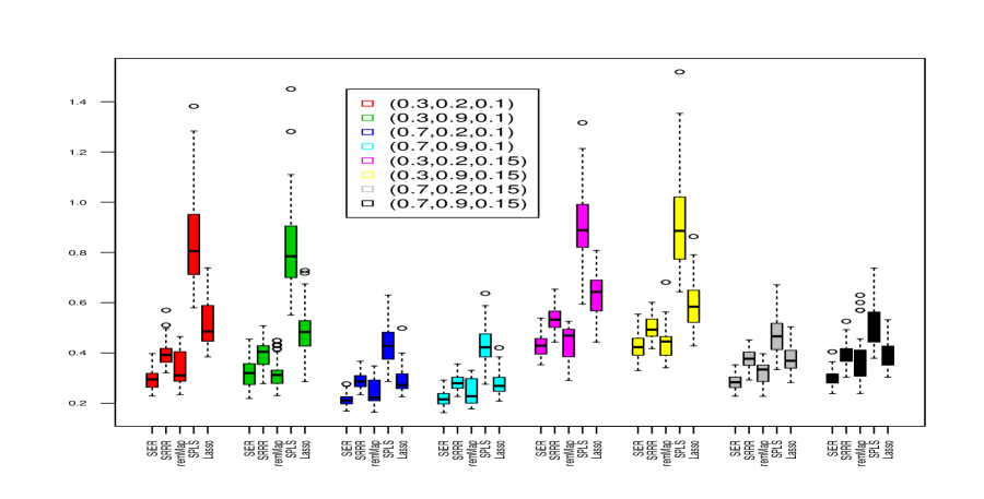
Figure 2: Boxplots of MSPE for different methods with different parameter settings $(\rho,r,q\sigma^{2})$ in Case 1 of the simulation studies.

Table 1: The averages and standard deviations (in parenthesis) of the MSPEs of 50 replicates for Case 1 in the simulation studies.

$q\sigma^{2}$	$\rho$	$r$	SiER	SRRR	RemMap	SPLS	SepLasso
0.1	0.3	0.2	0.295(0.039)	0.395(0.050)	0.336(0.067)	0.848(0.180)	0.504(0.087)
		0.9	0.320(0.053)	0.395(0.055)	0.322(0.060)	0.824(0.181)	0.489(0.088)
	0.7	0.2	0.214(0.023)	0.289(0.031)	0.244(0.051)	0.432(0.079)	0.289(0.049)
		0.9	0.217(0.028)	0.282(0.030)	0.243(0.050)	0.430(0.075)	0.282(0.047)
0.15	0.3	0.2	0.429(0.045)	0.536(0.049)	0.444(0.063)	0.918(0.137)	0.630(0.089)
		0.9	0.427(0.051)	0.501(0.045)	0.440(0.068)	0.923(0.202)	0.597(0.095)
	0.7	0.2	0.283(0.028)	0.376(0.037)	0.323(0.044)	0.475(0.079)	0.377(0.053)
		0.9	0.302(0.033)	0.394(0.046)	0.368(0.090)	0.508(0.089)	0.392(0.053)

5.2 Case 2

In this case and Case 3, we generate the coefficient matrix as the product of two lower rank matrices, $\mathcal{B}=CD$, where $C$ is a $p\times K$ matrix and $D$ is $K\times q$. In this case, we fix $K=3$ and choose $(p,q)=(100,20)$ or $(150,30)$. For the matrix $C$, each element in the first $p_{0}=40$ rows is independently generated from $N(0,1)$, the rest $p-p_{0}$ rows are set to be zero. Then each column of $C$ is scaled to unit norm. All elements in $D$ are first independently generated from the uniform distribution between $-1$ and $1$, and then each row of $D$ is scaled to unit norm. The first 50 predictors in $\mathbf{X}$ are generated from $N_{50}(0,\Sigma)$, where $\Sigma$ has diagonal elements 1 and off-diagonal elements $\rho$. All the other predictors are generated independently from $N(0,0.1^{2})$. The noise vector is generated from $N_{q}(0,\sigma^{2}R)$, where $R$ has diagonal elements 1 and off-diagonal elements $r$. We choose $\rho=0.3$ and 0.7, $q\sigma^{2}=0.015$ and $0.030$, $r=0$ and 0.5, and consider their all possible combinations. We show the average and standard deviation of MSPE in Table 2. The SiER has the smallest prediction errors in all the situations. The SRRR has a better prediction performance than RemMap because in this case, there are obvious reduced rank structure and row-wise sparsity structure. The MSPE of the first three methods are mostly affected by the magnitude of random error ($q\sigma^{2}$), and are less sensitive to the correlations of predictors and random errors, and the dimensions $p$ and $q$.

We also compare the dimension reduction and feature selection of all methods. The number of selected components, the sensitivity and specificity of variable selection are summarized in Table 3. Only three methods, the SiER, the SRRR and the SPLS, generate low rank latent components. In all settings, the SiER chooses the smallest number of components and is most efficient in dimension reduction. The SiER, SRRR and RemMap have sensitivity equal to one in all settings, that is, these three methods select all the true features. The SRRR has the highest specificity, and hence performs best in feature selection in this case. The SiER tends to select more features than the SRRR, the RemMap and the SPLS in this simulation setting.

Table 2: The averages and standard deviations (in parenthesis) of the MSPE for Case 2 in the simulation studies.

$(p,q)$	$q\sigma^{2}$	$\rho$	$r$	SiER	SRRR	RemMap	SPLS	SepLasso
(100,20)	0.015	0.3	0	0.020(0.009)	0.026(0.003)	0.038(0.005)	0.835(0.170)	0.175(0.054)
			0.5	0.020(0.005)	0.025(0.003)	0.037(0.005)	0.839(0.168)	0.167(0.049)
		0.7	0	0.019(0.001)	0.035(0.005)	0.043(0.004)	0.473(0.109)	0.268(0.057)
			0.5	0.019(0.002)	0.034(0.003)	0.041(0.004)	0.468(0.096)	0.272(0.075)
	0.030	0.3	0	0.037(0.001)	0.043(0.003)	0.063(0.001)	0.894(0.167)	0.241(0.066)
			0.5	0.040(0.017)	0.044(0.004)	0.070(0.010)	0.823(0.138)	0.230(0.056)
		0.7	0	0.038(0.002)	0.051(0.005)	0.069(0.005)	0.523(0.135)	0.306(0.068)
			0.5	0.037(0.003)	0.049(0.005)	0.069(0.007)	0.527(0.114)	0.298(0.060)
(150,30)	0.015	0.3	0	0.018(0.001)	0.025(0.003)	0.040(0.004)	1.015(0.172)	0.475(0.151)
			0.5	0.021(0.009)	0.025(0.003)	0.040(0.004)	0.953(0.165)	0.446(0.129)
		0.7	0	0.018(0.001)	0.033(0.004)	0.047(0.005)	0.599(0.117)	0.558(0.101)
			0.5	0.018(0.001)	0.032(0.003)	0.046(0.005)	0.603(0.110)	0.575(0.094)
	0.030	0.3	0	0.035(0.001)	0.042(0.003)	0.070(0.005)	0.972(0.185)	0.501(0.104)
			0.5	0.036(0.002)	0.042(0.004)	0.073(0.011)	1.023(0.183)	0.581(0.205)
		0.7	0	0.036(0.001)	0.050(0.005)	0.073(0.006)	0.625(0.164)	0.610(0.098)
			0.5	0.036(0.002)	0.049(0.005)	0.073(0.008)	0.628(0.171)	0.597(0.094)

Table 3: The average number ($\hat{K}$) of components selected for the SiER, SRRR and SPLS, and the sensitivity (Se) and specificity (Sp) of all methods in case 2 in the simulation studies.

$(p,q)$	$q\sigma^{2}$	$\rho$	$r$	SiER			SRRR			RemMap			SPLS			SepLasso
				$\hat{K}$	Se	Sp	$\hat{K}$	Se	Sp	$\hat{K}$	Se	Sp	$\hat{K}$	Se	Sp	$\hat{K}$	Se	Sp
(100,20)	0.015	0.3	0	3	1	0.58	3	1	0.92	–	1	0.83	5	0.77	0.84	–	0.76	0.25
			0.5	3	1	0.60	3	1	0.93	–	1	0.83	5	0.76	0.84	–	0.80	0.21
		0.7	0	3	1	0.33	3.22	1	0.94	–	1	0.83	5	0.94	0.77	–	0.20	0.80
			0.5	3	1	0.39	3.02	1	0.94	–	1	0.83	5	0.92	0.77	–	0.49	0.53
	0.030	0.3	0	3	1	0.59	3	1	0.90	–	1	0.83	5	0.78	0.80	–	1.00	0.00
			0.5	3	1	0.54	3	1	0.92	–	1	0.83	5	0.75	0.86	–	1.00	0.01
		0.7	0	3	1	0.47	3.06	1	0.93	–	1	0.81	4.92	0.94	0.74	–	1.00	0.02
			0.5	3	1	0.48	3.02	1	0.96	–	1	0.82	5	0.93	0.75	–	1.00	0.02
(150,30)	0.015	0.3	0	3	1	0.69	3	1	0.96	–	1	0.91	5	0.69	0.90	–	1.00	0.04
			0.5	3	1	0.71	3	1	0.96	–	1	0.91	4.98	0.70	0.89	–	1.00	0.04
		0.7	0	3	1	0.50	3.19	1	0.97	–	1	0.91	4.85	0.86	0.86	–	0.93	0.12
			0.5	3	1	0.57	3	1	0.97	–	1	0.91	4.85	0.83	0.87	–	0.92	0.14
	0.030	0.3	0	3	1	0.75	3	1	0.95	–	1	0.91	4.98	0.65	0.91	–	1.00	0.03
			0.5	3	1	0.71	3	1	0.95	–	1	0.91	4.98	0.73	0.89	–	1.00	0.05
		0.7	0	3	1	0.54	3.04	1	0.96	–	1	0.90	4.70	0.89	0.86	–	0.92	0.14
			0.5	3	1	0.58	3	1	0.96	–	1	0.90	4.77	0.80	0.86	–	0.92	0.12

5.3 Case 3

In this case, we still generate the coefficient matrix by $\mathcal{B}=CD$. We increase the dimensions $p$ and $q$, and introduce correlation among the coordinates of the row vectors of $D$. We take $K=3$, $p=1000$ or $2000$, $q=100$ or 200. The matrix $C$ is generated in the same way as in Case 2 with $p_{0}=100$. Each row of $D$ is first independently generated from the multivariate normal distribution $\hbox{N}_{q}(0,\Sigma_{D})$ and then scaled to have unit norm. The $(i,j)$-th element in $\Sigma_{D}$ is defined as $\hbox{exp}[-(|i-j|/100)^{\gamma}]$ for $i,j=1,\ldots,q$. Therefore, the row vectors of $D$ can be viewed as a discretely observed Gaussian process at time points $1/100,2/100,\cdots$. We choose $\gamma=1$ or 2 to represent different correlation levels, where $\gamma=2$ leads to a smoother Gaussian process than $\gamma=1$. The first 200 predictors in $\mathbf{X}$ are generated from $N_{200}(0,\Sigma)$, with the $(i,j)$-th element equal $\rho^{|i-j|}$ ($i,j=1,\ldots,200$). The rest $p-200$ predictors are independently generated from $N(0,0.1^{2})$. The random noise vector is generated from $N_{q}(0,\sigma^{2}R)$, where $R$ have diagonal elements 1 and off-diagonal elements 0.5. We fix $q\sigma^{2}=0.15$. We summarize the MSPE in Table 4, the dimension reduction and the sensitivity and specificity of variable selection in Table 5. In this case, the SRRR is not included because the heavy computation load makes it unavailable. As the noise level is fixed, the MSPE is not sensitive to $\gamma$, $p$ and $q$. The SiER has the lowest average MSPE among the four methods and choose less components than the SPLS. In this large dimension case, the SiER has both high sensitivity and high specificity.

Table 4: The averages and standard deviations (in parenthesis) of the MSPE for case 3.

$q$	$p$	$\gamma$	SiER	RemMap	SPLS	SepLasso
100	1000	1	1.739(0.185)	2.146(0.480)	2.816(0.370)	3.103(0.340)
		2	1.844(0.330)	2.264(0.615)	2.872(0.462)	3.117(0.501)
	2000	1	1.748(0.244)	2.108(0.485)	3.026(0.432)	3.202(0.408)
		2	1.740(0.337)	2.185(0.616)	2.944(0.396)	3.113(0.385)
200	1000	1	1.763(0.208)	2.180(0.419)	2.765(0.235)	3.131(0.488)
		2	1.774(0.304)	2.186(0.574)	2.843(0.320)	3.070(0.321)
	2000	1	1.756(0.224)	2.109(0.488)	2.960(0.279)	3.098(0.266)
		2	1.808(0.280)	2.243(0.611)	3.004(0.360)	3.161(0.354)

Table 5: The average number ($\hat{K}$) of components selected for the SiER and SPLS, and the sensitivity (Se) and specificity (Sp) of all methods in Case 3.

$q$	$p$	$\gamma$	SiER			RemMap			SPLS			SepLasso
			$\hat{K}$	Se	Sp	$\hat{K}$	Se	Sp	$\hat{K}$	Se	Sp	$\hat{K}$	Se	Sp
100	1000	1	2.86	0.84	0.93	–	0.77	0.93	3.44	0.45	0.77	–	0.42	0.86
		2	2.32	0.75	0.94	–	0.65	0.94	2.76	0.41	0.79	–	0.32	0.89
	2000	1	3	0.82	0.97	–	0.77	0.97	3.06	0.35	0.84	–	0.27	0.95
		2	2.40	0.76	0.97	–	0.65	0.97	2.38	0.30	0.85	–	0.23	0.95
200	1000	1	3.04	0.88	0.92	–	0.79	0.93	3.54	0.43	0.81	–	0.51	0.80
		2	2.34	0.78	0.93	–	0.71	0.93	2.70	0.35	0.83	–	0.39	0.85
	2000	1	2.96	0.85	0.97	–	0.81	0.96	3.26	0.35	0.83	–	0.37	0.91
		2	2.66	0.77	0.97	–	0.68	0.97	2.50	0.32	0.86	–	0.27	0.93

6 Application to the communities and crime data

The data set (Bache and Lichman, 2013) contains the socio-economic information about a large number of communities over the United States and the corresponding crime data. The goal is to predict different types of crimes of a community based on various socio-economic variables of the community such as the median family income, per capita number of police officers, and so on. We first remove the variables with a large proportion of missing. We also remove the response (crime) variables with too many zero values as it is not appropriate to treat them as continuous variables. Due to the high skewness of the variables, we use the logarithms of each of the original variables plus one as the new variables. After excluding samples with extreme values, we get 1514 samples and 102 predictors. The response variables are the transformed number of Assault, Burglary, Larceny, Auto Theft, and Arson, the transformed total number of violent crimes, and the transformed total number of non-violent crimes, per 100,000 population.

Figure 3: Boxplots of prediction errors for different methods in the study for the crime data.

Table 6: The frequency of the number of selected components ($\hat{K}$) and the mean (sd) of the number of selected features over 100 simulations for the crime data.

Methods	$\hat{K}$				number of selected features
	2	3	4	5
SiER	76	24	0	0	52.2(23.3)
SRRR	22	12	17	49	32.9(18.2)
RemMap	–	–	–	–	37.6(8.2)
SPLS	1	1	27	71	81.5(23.8)
SepLasso	–	–	–	–	32.7(7.4)

To evaluate the prediction performance and the selection of components and features, we repeat the following procedure 100 times: in each replicate, we randomly take 150 samples as training data, the remaining as test data, and apply all the five methods to the train data to build predictive models and obtain the MSPE by applying the model to the test data. The boxplots of prediction errors of all methods are shown in Figure 3. The mean MSPEs of the SiER and SPLS are close and smaller than others. Table 6 shows the frequency of the number of selected components and the mean and standard deviation of number of selected features for each method. The SiER selects two components in 76% of the 100 replicates and three components in all the other replicates. Both the SRRR and the SPLS tend to select more components and they select five components with the highest frequency.

Figure 4: Histograms of nonzero coefficients of variables that are selected over 90% times in predicting the number of assault.

Among the 100 replicates, 11 features are selected by the SiER over 90 times, such as the percentage of population who are divorced, the number of people living in urban areas, the percent of persons in dense housing, the number of kids born to never married, and so on. The histograms of nonzero coefficients of these variables for assault are shown in Figure 4. It can be seen that the percentage of kids in family housing with two parents (pctKids2Par) and the percentage of families with kids that are headed by two parents (pctFam2Par) have protective effects (with negative coefficients) in crime assault, and the other variables have positive associations with the number of assault. For other crime types, pctKids2Par and pctFam2Par also have protective effects. Percentages for divorce and dense housing, and the number of kids born to never married are positively associated with crimes. Coefficients for variables of population living in urban areas and having foreign born are positive for arson, but negative for auto theft.

7 Discussion

In this paper, we propose a signal extracting approach for dimension reduction and regression in multiple response linear model with high-dimensional predictor variables. Under the reduced rank assumptions on the coefficient matrix, we aim to estimate the optimal lower rank decomposition of the coefficient matrix in terms of approximating the regression function. We establish a general eigenvalue problem and its sparse version for high-dimensional settings. The solution of these problems provides the estimate of the first lower rank matrix. Applying the least squares regression on the response variables and new predictors generated from the estimate of the first lower rank matrix, we obtain the estimate of the second lower rank matrix. In the high-dimensional setting, we establish the oracle inequalities for the estimation of the lower rank matrices, the coefficient matrix and the estimated regression function, allowing correlation among random errors for different response variables. We do not make restrictions on the dimension of the multivariate response. In the special case of the usual linear regression model with a scalar response, our oracle inequalities provide upper bounds that have the same order as those for the Lasso and Dantzig selector. The simulation studies and the application to real data show that the proposed method has good prediction performance and is efficient in dimension reduction for various reduced rank models.

References

- Anderson (2002) Anderson, T. (2002) Specification and misspecification in reduced rank regression. Sankhyā: The Indian Journal of Statistics, Series A, 193–205.
- Bache and Lichman (2013) Bache, K. and Lichman, M. (2013) UCI machine learning repository. URL http://archive.ics.uci.edu/ml.
- Bickel and Levina (2008) Bickel, P. J. and Levina, E. (2008) Regularized estimation of large covariance matrices. The Annals of Statistics, 199–227.
- Bickel et al. (2009) Bickel, P. J., Ritov, Y. and Tsybakov, A. B. (2009) Simultaneous analysis of lasso and dantzig selector. The Annals of Statistics, 1705–1732.
- Bunea et al. (2011) Bunea, F., She, Y. and Wegkamp, M. H. (2011) Optimal selection of reduced rank estimators of high-dimensional matrices. The Annals of Statistics, 1282–1309.
- Bunea et al. (2012) Bunea, F., She, Y., Wegkamp, M. H. et al. (2012) Joint variable and rank selection for parsimonious estimation of high-dimensional matrices. The Annals of Statistics, 40, 2359–2388.
- Camba-Mendez et al. (2003) Camba-Mendez, G., Kapetanios, G., Smith, R. J. and Weale, M. R. (2003) Tests of rank in reduced rank regression models. Journal of Business & Economic Statistics, 21, 145–155.
- Chen et al. (2012) Chen, K., Chan, K.-S. and Stenseth, N. C. (2012) Reduced rank stochastic regression with a sparse singular value decomposition. Journal of the Royal Statistical Society: Series B (Statistical Methodology), 74, 203–221.
- Chen and Huang (2012) Chen, L. and Huang, J. Z. (2012) Sparse reduced-rank regression for simultaneous dimension reduction and variable selection. Journal of the American Statistical Association, 107, 1533–1545.
- Chun and Keles (2010) Chun, H. and Keles, S. (2010) Sparse partial least squares regression for simulatenous dimension reduction and variable selection. Journal of the Royal Statistical Society series B, 72, 3–25.
- Izenman (1975) Izenman, A. J. (1975) Reduced-rank regression for the multivariate linear model. Journal of multivariate analysis, 5, 248–264.
- Ledoux and Talagrand (2011) Ledoux, M. and Talagrand, M. (2011) Probability in Banach Spaces: Isoperimetry and Processes. Classics in Mathematics. Springer.
- Peng et al. (2010) Peng, J., Zhu, J., Bergamaschi, A., Han, W., Noh, D.-Y., Pollack, J. R. and Wang, P. (2010) Regularized multivariate regression for identifying master predictors with application to integrative genomics study of breast cancer. The annals of applied statistics, 4, 53.
- Qi et al. (2015) Qi, X., Luo, R., Carroll, R. J. and Zhao, H. (2015) Sparse regression by projection and sparse discriminant analysis. Journal of Computational and Graphical Statistics, 24, 416–438.
- Qi et al. (2013) Qi, X., Luo, R. and Zhao, H. (2013) Sparse principal component analysis by choice of norm. Journal of Multivariate Analysis, 114, 127–160.
- Reinsel and Velu (1998) Reinsel, G. C. and Velu, R. P. (1998) Multivariate reduced-rank regression. Springer.
- Similä and Tikka (2007) Similä, T. and Tikka, J. (2007) Input selection and shrinkage in multiresponse linear regression. Computational Statistics & Data Analysis, 52, 406–422.
- Turlach et al. (2005) Turlach, B. A., Venables, W. N. and Wright, S. J. (2005) Simultaneous variable selection. Technometrics, 47, 349–363.