Quasiparticle Interference in Fe-based Superconductors Based on a Five-Orbital Tight-Binding Model

Abstract

We investigate the quasiparticle interference (QPI) in Fe-based superconductors in both the $s_{++}$-wave and $s_{\pm}$-wave superconducting states on the basis of the five-orbital model. In the octet model for cuprate superconductors with $d_{x^{2}-y^{2}}$-wave state, the QPI signal due to the impurity scattering at $\bm{q}=\bm{k}_{i}-\bm{k}_{j}$ ($E=|\Delta(\bm{k}_{i})|$, $i=1\sim 8$) disappears when the gap functions at $\bm{k}_{i}$ and $\bm{k}_{j}$ have the same sign. However, we show that this extinction rule does not hold in Fe-based superconductors with fully-gapped $s$-wave state. The reason is that the resonance condition $E=|\Delta(\bm{k}_{i})|$ is not satisfied under the experimental condition for Fe-based superconductors. We perform the detailed numerical study of the QPI signal using the $T$-matrix approximation, and show that the experimentally observed QPI peak around $\bm{q}_{2}=(\pi,0)$ can be explained on the basis of both the $s_{++}$-wave and $s_{\pm}$-wave states. Furthermore, we discuss the magnetic field dependence of the QPI by considering the Zeeman effect, and find that the field-induced suppression of the peak intensity around $\bm{q}_{2}$ can also be explained in terms of both the $s_{++}$-wave and $s_{\pm}$-wave states.

I Introduction

Since the discovery of Fe-based superconductors, Kamihara much effort has been devoted to reveal the mechanism of high-$T_{\rm c}$ superconductivity (SC). The mother compounds exhibit structure and antiferromagnetic transitions. These transitions are suppressed by carrier doping and then the SC state emerges. In the early theoretical studies, spin fluctuation mediated $s_{\pm}$-wave state, in which the SC gap functions change their sign between the hole and electron Fermi surfaces (FS), was proposed. Kuroki ; Mazin ; Chubukov ; Graser ; Hirschfeld On the other hand, the orbital fluctuations can induce the $s_{++}$-wave state without sign change in the gap functions as discussed in Refs. Kontani, ; Saito, ; Onari, . Figure 1 shows the unfolded FS and schematic picture of the (a) $s_{++}$-wave and (b) $s_{\pm}$-wave states. The $s_{++}$($s_{\pm}$)-wave state is driven by the orbital (spin) fluctuations at $\bm{q}_{2}=(\pi,0)$ that corresponds to the nesting between hole and electron FSs.

To distinguish between the $s_{\pm}$-wave and $s_{++}$-wave states, various phase sensitive experiments have been performed, such as the impurity effect on $T_{\rm c}$, Sato ; Li ; Nakajima the resonant peak by the inelastic neutron scattering, Inosov the coherence peak by the nuclear magnetic resonance, Sato ; Nakai the quasiparticle interference (QPI) by the scanning tunneling microscope (STM), Hanaguri ; Hanaguri_arxiv ; Chi and so on. Many theorists have preformed theoretical investigations of such experiments based on the realistic five-orbital model. For example, the present authors have shown that the robustness of $T_{\rm c}$ against impurities is inconsistent with the $s_{\pm}$-wave state. Onari_imp ; Yamakawa_imp It has been shown that the broad resonant peak in the neutron scattering spectrum can be explained on the basis of the $s_{++}$-wave state rather than the $s_{\pm}$-wave state. Onari_neutron Also, the absence of the coherence peak at $T_{\rm c}$ can be explained in terms of both the $s_{++}$-wave and $s_{\pm}$-wave states. Yamakawa_nmr The theoretical study of the QPI signal in Fe-based superconductors ware performed by several theoretical groups in Refs. Sykora, ; Gao, ; Mazin_qpi, ; Zhang, ; Akbari, ; Das, ; Plamadeala, .

By using the STM measurement, the information of the local density of states can be obtained. The QPI signal $Z(\bm{q},E)$ is given by the Fourier transformation of the tunneling conductance ratio $Z(\bm{r},E)=\frac{dI/dV(\bm{r},+V)}{dI/dV(\bm{r},-V)}$ derived from the STM measurement. The QPI study played a crucial role to determine the pairing symmetry in cuprate superconductors. McElroy ; Hanaguri_Cu ; Maltseva In cuprate superconductors, the nodal $d_{x^{2}-y^{2}}$-wave SC state is realized. There are eight $\bm{k}$ points ($\bm{k}_{i}$ : $i=1\sim 8$) on the FS satisfying the relation $E=|\Delta(\bm{k}_{i})|$ for $E<\Delta^{\rm max}$. It is called the octet model, and the QPI signal $Z(\bm{q},E)$ with $\bm{q}=\bm{k}_{i}-\bm{k}_{j}$ emerges due to the impurity scattering when $\Delta(\bm{k}_{i})$ and $\Delta(\bm{k}_{j})$ have the opposite sign, while it disappears when $\Delta(\bm{k}_{i})$ and $\Delta(\bm{k}_{j})$ have the same sign. The disappearance of the QPI signal is called the “extinction rule”. Furthermore, the experimental QPI peak is rapidly suppressed by applying a magnetic field. The extinction rule and the magnetic field dependence of the QPI obtained in cuprate superconductors are well understood in terms of the octet model with $d_{x^{2}-y^{2}}$-wave gap symmetry.

In Fe-based superconductors, many experimental Hanaguri ; Hanaguri_arxiv ; Allan ; Hanke ; Chi ; Teague ; Cai and theoretical Sykora ; Gao ; Mazin_qpi ; Zhang ; Akbari ; Das ; Plamadeala studies of the STM have been performed. Hanaguri et al. carried out the QPI experiments on Fe(Se,Te) single crystal and reported the appearance of a shape peak around $\bm{q}_{2}=(\pi,0)$, Hanaguri ; Hanaguri_arxiv which is caused by the impurity scattering between hole and electron FSs. By analogy with the extinction rule in the octet model, the existence of the QPI peak around $\bm{q}_{2}$ may indicate that the gap functions on the hole and electron FSs have opposite sign, i.e., $s_{\pm}$-wave state. Although, many pioneering theoretical studies had been performed for Fe-based superconductors, some previous theoretical studies assumed over-simplified band structures. Furthermore, the QPI signal in the $s_{++}$-wave state had not been studied in detail in previous studies. Therefore, detailed theoretical study of the QPI based on a realistic five-orbital model in both the $s_{++}$-wave and $s_{\pm}$-wave states had been required.

Hanaguri et al. showed that the intensity of the QPI peak around $\bm{q}_{2}$ is slightly suppressed by the magnetic field $B=11$ T at $E=1.0$ meV. Hanaguri However, the field-induced change of the QPI peak around $\bm{q}_{2}$ non-monotonically depends on $E$; the peak intensity is slightly enhanced at $E=0.5$ meV and $E=1.9$ meV. [See Fig. 3S(I) in the Supplemental Material of Ref. Hanaguri, and Fig. 1(A) in Ref. Hanaguri_arxiv, .] Therefore, in this paper, we discuss the field-induced change of the QPI for wide range of $E$ in terms of both the $s_{++}$-wave and $s_{\pm}$-wave states.

In this paper, we investigate the QPI in Fe-based superconductors on the bases of both the $s_{++}$-wave and $s_{\pm}$-wave states. In the cuprate superconductors with $d_{x^{2}-y^{2}}$-wave SC state, the QPI signal at $\bm{q}=\bm{k}_{i}-\bm{k}_{j}$ disappears when $\Delta(\bm{k}_{i})$ and $\Delta(\bm{k}_{j})$ have the same sign. However, such extinction rule does not hold in Fe-based superconductors with fully-gapped $s$-wave SC state, since the resonance condition $E=|\Delta(\bm{k}_{i})|=|\Delta(\bm{k}_{j})|$ is not satisfied under the experimental condition $E<\Delta^{\rm min}$ regardless of the sign of the gap functions. We perform the detailed numerical study of the QPI signal based on the five-orbital model, and find that the experimentally observed QPI peak around $\bm{q}_{2}=(\pi,0)$ appears in both the $s_{++}$-wave and $s_{\pm}$-wave states. Furthermore, we discuss the magnetic field dependence of the QPI by considering the Zeeman effect, and find that the field-induced change of the peak intensity around $\bm{q}_{2}$ can also be explained in terms of both the $s_{++}$-wave and $s_{\pm}$-wave states. In conclusion, it is difficult to distinguish between the $s_{++}$-wave and $s_{\pm}$-wave states from the QPI experiments in Fe-based superconductors.

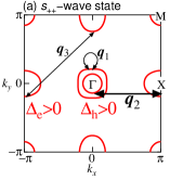
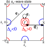
Figure 1: (Color online) Fermi surfaces and gap structures in the (a) $s_{++}$-wave and (b) $s_{\pm}$-wave states. The arrows denote scattering wave vectors. The scattering vector $\bm{q}_{2}\sim(\pi,0)$, which is equal to the nesting vector, connects hole and electron Fermi pockets. $\bm{q}_{1}\sim(0,0)$ corresponds to the intra-band scattering, and $\bm{q}_{3}\sim(\pi,\pi)$ corresponds to the scattering within electron or hole Fermi pockets.

II Formulation

II.1 Quasiparticle Interference

The tunneling conductance $dI/dV(\bm{r},V)$ at position $\bm{r}$ and voltage $V$ is approximately proportional to the local density of states $\rho(\bm{r},E)$ at energy $E=V$, namely, $dI/dV(\bm{r},V)\propto\left|M(\bm{r})\right|^{2}\rho(\bm{r},E)$, where we set the unit of charge $e$ as one. $M(\bm{r})$ is the tunneling matrix element between the sample surface and the STM tip. In the presence of the impurities, we can drop the factor $M(\bm{r})$ and obtain the information of the density of states by taking the ratio $Z(\bm{r},E)$ between the conductance measured at $+V$ and $-V$ as follows: Maltseva ; Sykora

$$\ Z(\bm{r},E) \equiv \frac{dI/dV(\bm{r},+V)}{dI/dV(\bm{r},-V)}=\frac{\rho(\bm{r},+E)}{\rho(\bm{r},-E)}$$ (1)

$$\approx \frac{\rho^{0}(+E)}{\rho^{0}(-E)}\left[1+\frac{\delta\rho(\bm{r},+E)}{\rho^{0}(\bm{r},+E)}-\frac{\delta\rho(\bm{r},-E)}{\rho^{0}(\bm{r},-E)}\right],$$

where $\rho^{0}(E)$ is the averaged density of states and $\delta\rho(\bm{r},E)$ describes the spatial modulation defined as $\delta\rho(\bm{r},E)\equiv\rho(\bm{r},E)-\rho^{0}(E)$. The Fourier transformed conductance ratio is called the QPI signal, which is given by

$$Z(\bm{q},E)=\frac{\rho^{0}(+E)}{\rho^{0}(-E)} \bigg{[}(2\pi)^{2}\delta(\bm{q})$$ (2)

$$+\frac{\delta\rho(\bm{q},+E)}{\rho^{0}(+E)}-\frac{\delta\rho(\bm{q},-E)}{\rho^{0}(-E)}\bigg{]},$$

where $\bm{q}$ is a scattering wave vector. When the system is uniform, $Z(\bm{q},E)$ is zero except for $\bm{q}=0$. We can obtain the information on the SC gap symmetry since the momentum dependence of $Z(\bm{q},E)$ reflects the sign of the gap functions.

II.2 Model Hamiltonian and Green Function

The five-orbital tight-binding Hamiltonian is given by

$$\mathcal{H}^{0}=\sum_{\bm{k},l,l^{\prime},\sigma}H_{\bm{k},l,l^{\prime}}^{0}c_{\bm{k},l,\sigma}^{\dagger}c_{\bm{k},l^{\prime},\sigma}$$ (3)

where $c_{\bm{k},l,\sigma}^{\dagger}$ ($c_{\bm{k},l,\sigma}$) is the creation (annihilation) operator of a Fe $3d$ electron with wave vector $\bm{k}$, orbital $l$ and spin $\sigma$. $\hat{H}_{\bm{k}}^{0}$ is given by the Fourier transformation of the hopping integrals introduced in Ref. Kuroki, . The energy dispersion $\epsilon_{\bm{k},b}$ of band $b$ is obtained as a eigenvalue of $\hat{H}_{\bm{k}}^{0}$ by unitary transformation,

$$\epsilon_{\bm{k},b}=\sum_{l,l^{\prime}}U_{\bm{k},l,b}^{*}H_{\bm{k},l,l^{\prime}}^{0}U_{\bm{k},l^{\prime},b},$$ (4)

where $U_{\bm{k},l,b}$ is an element of the unitary matrix obtained as the eigenvector. The obtained Fermi Surface is shown in Fig. 1.

Now we study the SC state. In a single-orbital model, the BCS Hamiltonian is simply given by

$$\mathcal{H} = \sum_{\bm{k}}\hat{\Psi}_{\bm{k}}^{\dagger}\hat{H}_{\bm{k}}\hat{\Psi}_{\bm{k}},$$ (5)

where

$$\hat{\Psi}_{\bm{k}}^{\dagger}\equiv\left(c_{\bm{k},\uparrow}^{\dagger},c_{-\bm{k},\downarrow}^{\dagger},c_{-\bm{k},\downarrow},-c_{\bm{k},\uparrow}\right).$$ (6)

Here, we define the Pauli matrices $\hat{\tau}_{i}$ and $\hat{\sigma}_{i}$ which act in particle-hole space and spin space, respectively. For example,

$$\hat{\tau}_{1} = \left(\begin{array}[]{cccc}0&0&1&0\\ 0&0&0&1\\ 1&0&0&0\\ 0&1&0&0\end{array}\right),\quad\hat{\tau}_{3}=\left(\begin{array}[]{cccc}1&0&0&0\\ 0&1&0&0\\ 0&0&-1&0\\ 0&0&0&-1\end{array}\right),$$ (15)

$$\hat{\sigma}_{3} = \left(\begin{array}[]{cccc}1&0&0&0\\ 0&-1&0&0\\ 0&0&1&0\\ 0&0&0&-1\end{array}\right).$$ (20)

Then, the Nambu Hamiltonian $\hat{H}_{\bm{k}}$ for a single-orbital model is given by

$$\hat{H}_{\bm{k}}=\epsilon_{\bm{k}}\hat{\tau}_{3}-B\hat{\sigma}_{3}+\Delta_{\bm{k}}\hat{\tau}_{1},$$ (21)

where $B$ is the Zeeman splitting energy by the magnetic field and $\Delta_{\bm{k}}$ is the singlet gap function.

In the five-orbital model, the Nambu Hamiltonian is written as follows:

$$\hat{H}_{\bm{k}}=\hat{H}_{\bm{k}}^{0}\hat{\tau}_{3}-B\hat{E}_{5}\hat{\sigma}_{3}+\hat{\Delta}^{\rm orb}_{\bm{k}}\hat{\tau}_{1},$$ (22)

where $\hat{E}_{5}$ is the $5\times 5$ unit matrix in the orbital space. In the case of the five-orbital model, the Nambu Hamiltonian is given by the $20\times 20$ matrix form. $\hat{\Delta}^{\rm orb}_{\bm{k}}$ is $5\times 5$ matrix form singlet gap function in the orbital space, and its matrix element is obtained by the unitary transformation of the band-basis gap function $\Delta_{\bm{k},b}$ as

$$\Delta^{\rm orb}_{\bm{k},l,l^{\prime}}\equiv\sum_{b}U_{\bm{k},l,b}\Delta_{\bm{k},b}U_{\bm{k},l^{\prime},b}^{*}.$$ (23)

Then, the Green function in the clean limit is given by

$$\hat{G}^{0}_{\bm{k}}(\omega) = \left(\omega-\hat{H}_{\bm{k}}\right)^{-1}$$ (24)

$$= \left(\omega-\hat{H}_{\bm{k}}^{0}\hat{\tau}_{3}+B\hat{E}_{5}\hat{\sigma}_{3}-\hat{\Delta}^{\rm orb}_{\bm{k}}\hat{\tau}_{1}\right)^{-1},$$

and the local density of states without randomness is given by

$$\rho^{0}(\omega)=-\frac{1}{\pi N}\sum_{\bm{k}}{\rm ImTr}\hat{E}_{5}\frac{\hat{\tau}_{0}+\hat{\tau}_{3}}{2}\left.\hat{G}^{0}_{\bm{k}}(\bar{\omega})\right|_{\bar{\omega}=\omega+i\gamma},$$ (25)

where $\gamma$ is the quasiparticle damping rate.

When we consider the impurity scattering, the Green function is obtained by using the $T$-matrix approximation as follows:

$$\hat{G}_{\bm{k},\bm{k}^{\prime}}(\omega)=\hat{G}^{0}_{\bm{k}}(\omega)\delta_{\bm{k},\bm{k}^{\prime}}+\delta\hat{G}_{\bm{k},\bm{k}^{\prime}}(\omega),$$ (26)

where

$$\delta\hat{G}_{\bm{k},\bm{k}^{\prime}}(\omega)\equiv\hat{G}^{0}_{\bm{k}}(\omega)\hat{T}_{\bm{k},\bm{k}^{\prime}}(\omega)\hat{G}^{0}_{\bm{k}^{\prime}}(\omega).$$ (27)

For a single impurity, the $T$-matrix is obtained by solving the following self-consistent equation,

$$\hat{T}_{\bm{k},\bm{k}^{\prime}}(\omega)=\hat{I}_{\bm{k},\bm{k}^{\prime}}+\frac{1}{N}\sum_{\bm{k}"}\hat{I}_{\bm{k},\bm{k}"}\hat{G}^{0}_{\bm{k}"}(\omega)\hat{T}_{\bm{k}",\bm{k}^{\prime}}(\omega),$$ (28)

where $\hat{I}_{\bm{k},\bm{k^{\prime}}}$ is the impurity potential of a single impurity. The modulation of the density of states induced by the impurity scattering is given by Maltseva ; Sykora

$$\delta\rho(\bm{q},\omega)=-\frac{n^{\rm imp}}{\pi N}\sum_{\bm{k}}{\rm ImTr}\hat{E}_{5}\frac{\hat{\tau}_{0}+\hat{\tau}_{3}}{2}\left.\delta\hat{G}_{\bm{k},\bm{k+q}}(\bar{\omega})\right|_{\bar{\omega}=\omega+i\gamma},$$ (29)

where $\hat{G}$ is represented in the orbital basis. This treatment is exact for the case of low impurity concentration $n^{\rm imp}\ll 1$.

In this paper, we consider the non-magnetic impurity since the QPI due to the magnetic impurity scattering is subdominant for $B=0$. Sykora According to the band calculations, the impurity potential in Fe-based superconductors is screened and well-localized. Nakamura That is, the impurity scattering matrix in the orbital space is $\bm{k}$-independent. When the Fe-site substitution is considered, the impurity potential is given as

$$\hat{I}^{\rm imp}=I^{\rm imp}\hat{E}_{5}\hat{\tau}_{3},$$ (30)

and then, the $T$-matrix becomes $\bm{k}$-independent and it is simply given by

$$\hat{T}(\omega)=\left(1-\hat{I}^{\rm imp}\hat{g}^{0}(\omega)\right)^{-1}\hat{I}^{\rm imp},$$ (31)

where $\hat{g}^{0}(\omega)\equiv\frac{1}{N}\sum_{\bm{k}}\hat{G}^{0}_{\bm{k}}(\omega)$ is the local Green function in the $20\times 20$ matrix form.

III Result

III.1 Simple Analytical Calculation

In this section, we analytically show that the extinction rule, which tells that the non-magnetic impurity scattering between FSs with same sign gap functions does not contribute to the QPI, does not hold in fully gapped $s$-wave SC state.

Here, we verify the case with the particle-hole symmetry $\rho^{0}(+E)=\rho^{0}(-E)$. Then, $Z(\bm{q},E)$ in Eq. (2) is simplified as

$$Z(\bm{q}\neq\bm{0},E)=\frac{2\delta\rho^{\rm odd}(\bm{q},E)}{\rho^{0}(E)},$$ (32)

where

$$\delta\rho^{\rm odd}(\bm{q},E)\equiv\frac{\delta\rho(\bm{q},+E)-\delta\rho(\bm{q},-E)}{2}.$$ (33)

When we consider the scattering due to non-magnetic impurities with a weak scalar potential $I^{\rm imp}$, the $T$-matrix is given by $\hat{T}\approx I^{\rm imp}\hat{E}_{5}\hat{\tau}_{3}$. From Eq. (29), the modulation of the density of states for $\hat{T}\approx I^{\rm imp}\hat{E}_{5}\hat{\tau}_{3}$ is given by

$$\delta\rho^{\rm odd}(\bm{q},E)=-\frac{n^{\rm imp}}{\pi N}\sum_{\bm{k}}{\rm ImTr}\hat{E}_{5}\frac{\hat{\tau}_{3}}{2}\delta\hat{G}_{\bm{k},\bm{k}+\bm{q}}(\bar{E})\Big{|}_{\bar{E}=E+i\gamma}$$ (34)

$$\approx -\frac{n^{\rm imp}I^{\rm imp}}{2\pi N}\sum_{\bm{k},b,b^{\prime}}{\rm Im}\left.\frac{\bar{E}^{2}+\epsilon_{\bm{k},b}\epsilon_{\bm{k}+\bm{q},b^{\prime}}-\Delta_{\bm{k},b}\Delta_{\bm{k}+\bm{q},b^{\prime}}}{(\bar{E}^{2}-E_{\bm{k},b}^{2})(\bar{E}^{2}-E_{\bm{k}+\bm{q},b^{\prime}}^{2})}\right|_{\bar{E}=E+i\gamma}$$

$$\times\left|\sum_{l}U_{\bm{k},l,b}U_{\bm{k}+\bm{q},l,b^{\prime}}^{*}\right|^{2}.$$

In the last line, we utilized the functional form of the Green function in the band-diagonal basis, and $E_{\bm{k},b}^{2}\equiv\epsilon_{\bm{k},b}^{2}+\Delta_{\bm{k},b}^{2}$ is the energy of a quasiparticle in band $b$. In Eq. (34), the main contribution originates from the case that both $\bm{k}$ and $\bm{k}+\bm{q}$ are on FSs ($\epsilon_{\bm{k},b}=\epsilon_{\bm{k}+\bm{q},b^{\prime}}=0$). In this case, the contribution is simplified as

$$\delta\rho^{\rm odd}(\bm{q},E)\propto-\!\!\!\!\sum_{\bm{k},\bm{k}+\bm{q}\in{\rm FS}}\!\!\!\!{\rm Im}\left.\frac{\bar{E}^{2}-\Delta_{\bm{k}}\Delta_{\bm{k}+\bm{q}}}{(\bar{E}^{2}-\Delta_{\bm{k}}^{2})(\bar{E}^{2}-\Delta_{\bm{k}+\bm{q}}^{2})}\right|_{\bar{E}=E+i\gamma}.$$ (35)

In cuprate superconductors, the nodal $d_{x^{2}-y^{2}}$-wave SC state is realized. Under the experimental condition $E<\Delta^{\rm max}$, only the eight $\bm{k}$ points ($\bm{k}_{i}$ : $i=1\sim 8$) satisfy the relation $E=|\Delta_{\bm{k}_{i}}|$. It is called the octet model,McElroy ; Hanaguri_Cu ; Maltseva and $\bm{k}_{1}\sim\bm{k}_{8}$ are shown in Fig. 6(a). $\delta\rho^{\rm odd}(\bm{q},E)$ can be very large for $\bm{q}=\bm{k}_{i}-\bm{k}_{j}$ since the denominator in Eq. (35) is almost zero for $\bm{k}\approx\bm{k}_{i}$. On the other hand, the numerator is sensitive to the sign of the gap functions: the numerator has finite value $2E^{2}$ when the gap functions $\Delta_{\bm{k}}$ and $\Delta_{\bm{k}+\bm{q}}$ have opposite sign, but it becomes zero for the same sign case. Therefore, the QPI peak disappears when the gap functions at $\bm{k}$ and $\bm{k}+\bm{q}$ have the same sign, which is called the extinction rule.

In contrast, such extinction rule does not hold in the fully gapped $s$-wave SC state realized in Fe-based superconductors, under the experimental condition $E<\Delta^{\rm min}$. We focus on the QPI peak around $\bm{q}_{2}=(\pi,0)$ which corresponds to the inter-band scattering between the hole and electron FSs. Using the gap functions on hole FS $\Delta_{\rm h}$ and electron FS $\Delta_{\rm e}$, $\delta\rho^{\rm odd}(\bm{q}_{2},E)$ is given by

$$\delta\rho^{\rm odd}(\bm{q}_{2},E)\propto-{\rm Im}\left.\frac{\bar{E}^{2}-\Delta_{\rm h}\Delta_{\rm e}}{(\bar{E}^{2}-\Delta_{\rm h}^{2})(\bar{E}^{2}-\Delta_{\rm e}^{2})}\right|_{\bar{E}=E+i\gamma}.$$ (36)

In the case of $E<|\Delta_{\rm h,e}|$, both the numerator and denominator have finite value regardless of the signs of $\Delta_{\rm h}$ and $\Delta_{\rm e}$. That is, $\delta\rho^{\rm odd}(\bm{q}_{2},E)$ is finite even for $\Delta_{\rm h}\Delta_{\rm e}>0$. Therefore, the extinction rule does not hold in Fe-based superconductors, and the QPI peak around $\bm{q}_{2}$ is expected to appear in both the $s_{++}$-wave and $s_{\pm}$-wave states. We will numerically verify the violation of the extinction rule for the $\bm{q}_{2}$ signal by analyzing the five-orbital model in later sections.

As shown in Fig. 1, the other QPI signal can arise around $\bm{q}_{1}=(0,0)$ due to intra-band scattering, and around $\bm{q}_{3}=(\pi,\pi)$ due to inter-band scattering between hole-FSs or electron-FSs. Experimentally, the QPI peak around $\bm{q}_{3}$ is enhanced by the external magnetic field. However, both the QPI peaks around $\bm{q}_{1}$ and $\bm{q}_{3}$ are caused by the scattering between hole-pockets and between electron-pockets. These QPI peaks are not useful for the purpose of distinguishing between the $s_{++}$-wave and $s_{\pm}$-wave states.

III.2 QPI for the Weak Impurity Potential Case

In this and subsequent sections, we numerically calculate the QPI signal using Eq. (29). Here, we discuss the QPI due to a weak impurity potential $I^{\rm imp}=0.1$ eV, and show that the QPI peak around $\bm{q}_{2}$ is actually obtained in both the $s_{++}$-wave and $s_{\pm}$-wave states for various parameters. Hereafter, we set $\Delta_{0}=0.02$ eV, $n^{\rm imp}=0.01$, $\gamma=\Delta_{0}/4$ and $N=256\times 256$. We confirmed that the obtained results do not change qualitatively for $\gamma=\Delta_{0}/8$.

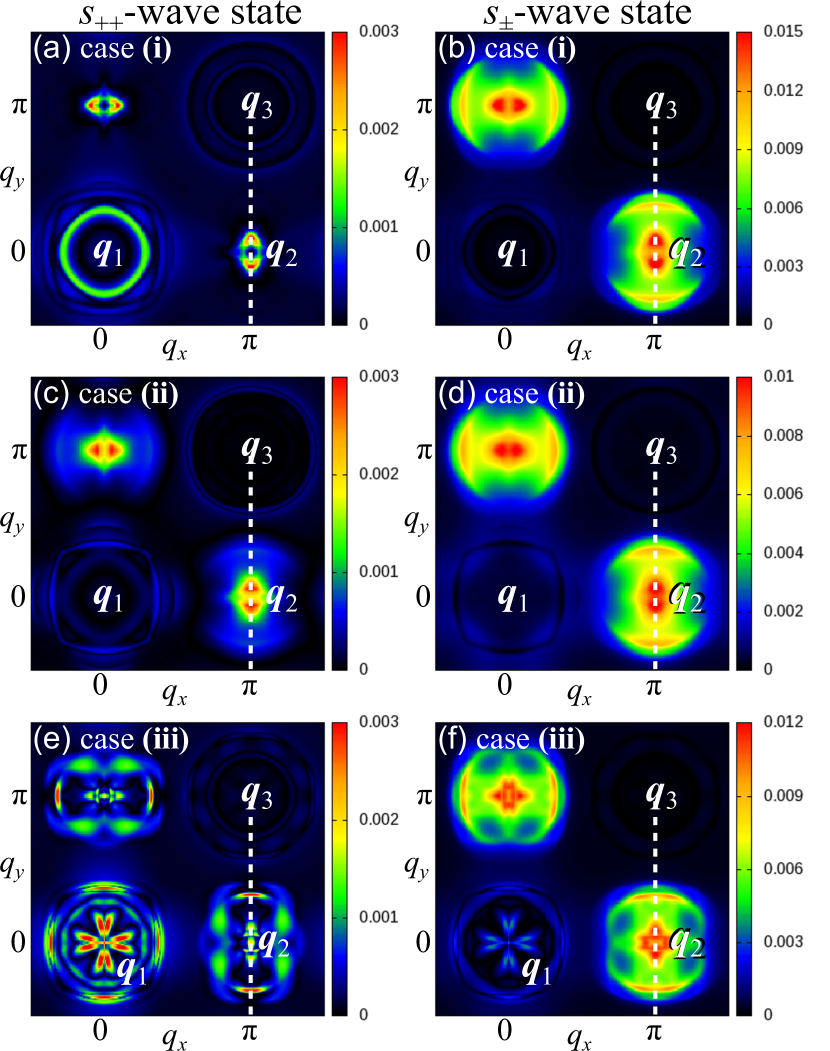
Figure 2: (Color online) Intensity map of the QPI $|Z(\bm{q},E)|$ under zero field $B=0$ at $E=\Delta_{0}/2$ due to the non-magnetic impurity scattering with potential $I^{\rm imp}=0.1$ eV. The left and right panels show the results in the $s_{++}$-wave and $s_{\pm}$-wave states, respectively. (a),(b) Case (i): Isotropic single-gap case with $\Delta_{\rm h}=\pm\Delta_{\rm e}=\Delta_{0}$. (c),(d) Case (ii): Isotropic two-gap case with $\Delta_{\rm h}=2\Delta_{0}$ and $\Delta_{\rm e}=\pm\Delta_{0}$. (e),(f) Case (iii): Strongly anisotropic gap case with $\Delta_{\rm h}=\Delta_{0}$, $\Delta_{\rm e}=\pm(1+\cos 2\theta)\Delta_{0}$ around $\bm{k}=(\pi,0)$ and $\Delta_{\rm e}=\pm(1-\cos 2\theta)\Delta_{0}$ around $\bm{k}=(0,\pi)$. The vertical broken lines represent the path of the linecuts in Fig. 3.

Figure 2 shows the intensity map of the QPI, $|Z(\bm{q},E)|$, at zero field. First, we discuss the (i) isotropic single-gap case with $|\Delta_{\rm h}|=|\Delta_{\rm e}|=\Delta_{0}$: Figures 2(a) and (b) show the results obtained in the $s_{++}$-wave and $s_{\pm}$-wave states, respectively. Considering the experimental condition in Ref. Hanaguri, , we set $E=\Delta_{0}/2$. In the $s_{++}$-wave state (a), the sharp QPI peak around $\bm{q}_{2}$ clearly appears as expected from Eq. (36). Therefore, the extinction rule does not hold in Fe-based superconductors. In the $s_{\pm}$-wave state (b), the strong QPI peak accompanied by the large halo structure is obtained around $\bm{q}_{2}$. That is, it is difficult to distinguish between the $s_{++}$-wave and $s_{\pm}$-wave states by the presence or absence of the QPI peak around $\bm{q}_{2}$.

In reality, $|\Delta_{\rm h}|$ and $|\Delta_{\rm e}|$ are different in usual Fe-based superconductors. For example, $|\Delta^{\rm max}/\Delta^{\rm min}|\sim 2$ is reported in electron- and hole-doped BaFe₂As₂. Williams ; Nakayama In the Fe(Se,Te) sample used in the QPI experiments, Hanaguri the relations $\Delta_{\rm min}\sim 1$ meV and $\Delta_{\rm max}=2\sim 4$ are expected from the tunneling conductance measurement. Therefore, we show the results for the (ii) isotropic two-gap case with $|\Delta_{\rm h}|=2\Delta_{0}$ and $|\Delta_{\rm e}|=\Delta_{0}$ in Figs. 2(c) and (d). In this case, there is no large difference from the single-gap case shown in Figs. 2(a) and (b). Similar results are obtained when $|\Delta_{\rm h}|=\Delta_{0}$ and $|\Delta_{\rm e}|=2\Delta_{0}$.

In Figs. 2(e) and (f), we also show the (iii) strongly anisotropic gap case with $|\Delta_{\rm h}|=\Delta_{0}$ and $|\Delta_{\rm e}|=(1\pm\cos 2\theta)\Delta_{0}$. Anisotropic-gap functions are reported on a hole-FS in heavily K-doped BaFe₂As₂ Ota and on the electron FSs in some Fe(Se,Te) systems. Zeng ; Song In this case, the peak around $\bm{q}_{2}$ exists and its shape in the $s_{++}$-wave state becomes similar to the one in the $s_{\pm}$-wave state. Therefore, it is difficult to distinguish between the $s_{++}$-wave and $s_{\pm}$-wave states from the existence of the QPI signal around $\bm{q}_{2}$.

Experimentally, the QPI peak intensity around $\bm{q}_{2}$ is slightly suppressed by the magnetic field $B$ for $E=1.0$ meV $\leq\Delta^{\rm min}$. Hanaguri ; Hanaguri_arxiv Here, we discuss $B-$ and $E-$ dependencies of $|Z(\bm{q},E)|$ in detail, and show that the experimental suppression of the $\bm{q}_{2}$ peak for $E\sim\Delta^{\rm min}$ can be explained in both the $s_{++}$-wave and $s_{\pm}$-wave states. Previously, two kinds of the field-induced suppression effects have been discussed by Coleman et al.: Sykora ; Maltseva (A) Impurities are masked by vortices under the magnetic field, and then the impurity scattering rate is reduced. Also, (B) the Zeeman effect changes the electronic state and modifies the impurity scattering. The former mechanism would suppress the QPI intensity around $\bm{q}_{2}$ regardless of the sign of the gap functions. However, in the QPI experiments for Fe(Se,Te) in Ref. Hanaguri, , it was reported that the effect (B) would be dominant, since the field-induced changes are almost spatially uniform. Therefore, in this paper, we study only the effect (B).

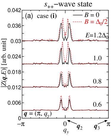
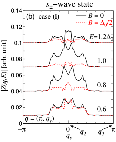
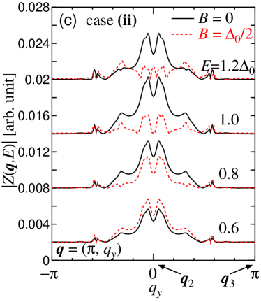
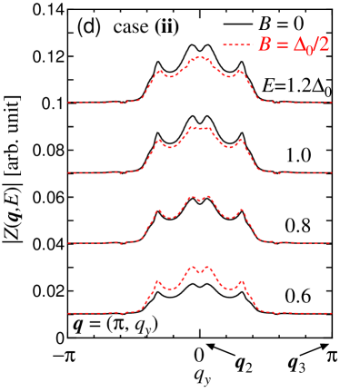
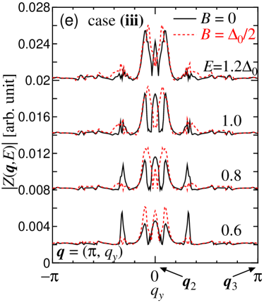
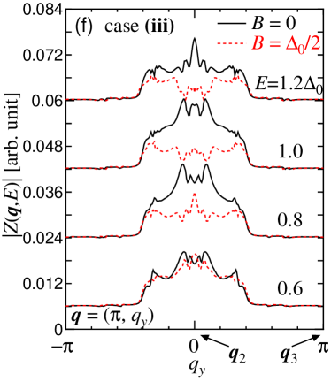
Figure 3: (Color online) Linecuts from $|Z(\bm{q},E)|$ map for $I^{\rm imp}=0.1$ eV. The solid and dotted lines represent $|Z(\bm{q},E)|_{B=0}$ and $|Z(\bm{q},E)|_{B=\Delta_{0}/2}$, respectively. The left and right panels show the results in the $s_{++}$-wave and $s_{\pm}$-wave states, respectively. The path is shown in Fig. 2. (a),(b) Case (i): Isotropic single-gap case with $\Delta_{\rm h}=\pm\Delta_{\rm e}=\Delta_{0}$. (c),(d) Case (ii): Isotropic two-gap case with $\Delta_{\rm h}=2\Delta_{0}$ and $\Delta_{\rm e}=\pm\Delta_{0}$. (e),(f) Case (iii): Strongly anisotropic gap case with $\Delta_{\rm h}=\Delta_{0}$, $\Delta_{\rm e}=\pm(1+\cos 2\theta)\Delta_{0}$ around $\bm{k}=(\pi,0)$ and $\Delta_{\rm e}=\pm(1-\cos 2\theta)\Delta_{0}$ around $\bm{k}=(0,\pi)$. The curves in all the figures are vertically shifted to make them visible.

Figures 3(a) and (b) show the $|Z(\bm{q},E)|$ in the single-gap case with $|\Delta_{\rm h}|=|\Delta_{\rm e}|=\Delta_{0}$ [case (i)] from $\bm{q}=(\pi,-\pi)$ to $(\pi,\pi)$. The path is shown in Fig. 2 by the vertical dashed lines. The solid and dotted lines represent the results for $B=0$ and $B=\Delta_{0}/2$, respectively. In the (a) $s_{++}$-wave state, the QPI peak around $\bm{q}_{2}$ is not sensitive to $B$ and $E$. On the other hand, in the (b) $s_{\pm}$-wave state, the $\bm{q}_{2}$ peak is drastically suppressed by $B$. Figures 3(c) and (d) show the results obtained for the two-gap case [case (ii)]. In this case, the QPI peak around $\bm{q}_{2}$ is suppressed by $B$ for $E\sim\Delta_{0}$ in both the $s_{++}$-wave and $s_{\pm}$-wave states. However, the field suppression of the QPI peaks is much larger in the $s_{++}$-wave state. Figures 3(e) and (f) show the results for the strongly anisotropic gap case [case (iii)]. In this case, $|Z(\bm{q},E)|$ in the $s_{++}$-wave state shows very complex $B$ dependence.

In summary, in the $s_{\pm}$-wave state, the QPI peak around $\bm{q}_{2}$ is clearly suppressed in all cases (i)-(iii). In the $s_{++}$-wave state, this peak intensity is also suppressed in the two-gap case (ii). Therefore, the field-induced suppression of the QPI around $\bm{q}_{2}$ can be explained in terms of both the $s_{++}$-wave and $s_{\pm}$-wave states. Experimentally, the SC gaps are fully opened in the Fe(Se,Te) sample used for the QPI experiments, and relation $\Delta^{\rm max}\gg\Delta^{\rm min}\sim 1$ meV is expected, since the estimated value of $2\Delta^{\rm min}/T_{\rm c}<2$ is much smaller than the BCS value $3.53$. In addition, the tunneling conductance has the sharp gap edge peak at $V\approx 1.7$ mV and an additional peak at about $4$ mV. If the latter peak arises from the SC gap, $\Delta^{\rm max}/\Delta^{\rm min}\geq 2$ is expected. Therefore, the isotropic two-gap case with $|\Delta_{\rm h}|=2|\Delta_{\rm e}|$ [case (ii)] would correspond to Fe(Se,Te).

III.3 QPI for the Strong Impurity Potential Case

In this section, we consider the QPI due to a strong impurity potential $|I^{\rm imp}|=1$ eV, which corresponds to Fe-site substitution. Since the residual resistivity takes the maximum for $I^{\rm imp}\sim+1$ eV, $I^{\rm imp}=+1$ eV corresponds to the unitary limit in Fe-based superconductors. Onari_imp ; Yamakawa_imp Here, we show the result only for the isotropic two-gap case with $|\Delta_{\rm h}|=2\Delta_{0}$ and $|\Delta_{\rm e}|=\Delta_{0}$ [case (ii)].

Figures 4(a) and (b) show the $|Z(\bm{q},E)|$ map for $I^{\rm imp}=-1$ eV in the case of the $s_{++}$-wave and $s_{\pm}$-wave states, respectively. Also, Figs. 4(c) and (d) show the ones for $I^{\rm imp}=+1$ eV. We set $E=\Delta_{0}/2$ and $B=0$. The obtained QPI map is qualitatively similar to the ones in the weak potential case shown in Fig. 2, and the QPI peak around $\bm{q}_{2}$ appears in both the $s_{++}$-wave and $s_{\pm}$-wave states. Therefore, the extinction rule does not hold in Fe-based superconductors regardless of the magnitude of the impurity potential.

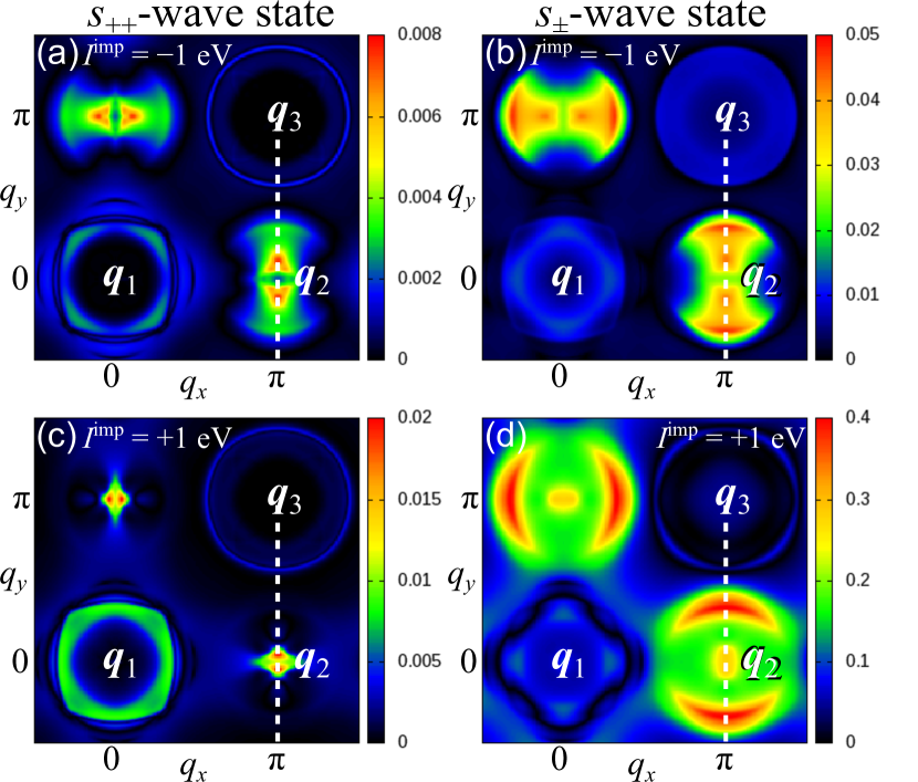
Figure 4: (Color online) Intensity map of $|Z(\bm{q},E)|$ at $E=\Delta_{0}/2$ and $B=0$ in the isotropic two-gap case with $\Delta_{\rm h}=2\Delta_{0}$ and $\Delta_{\rm e}=\pm\Delta_{0}$ [case (ii)]. The left and right panels show the results in the $s_{++}$-wave and $s_{\pm}$-wave states, respectively. (a),(b) $I^{\rm imp}=-1$ eV. (c),(d) $I^{\rm imp}=+1$ eV. The vertical broken lines represent the path of the linecuts in Fig. 5.

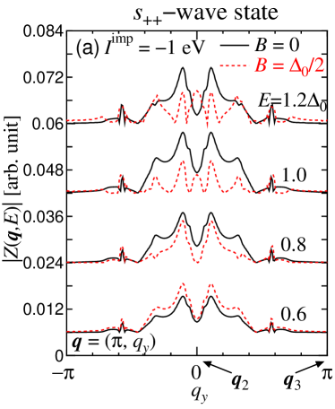
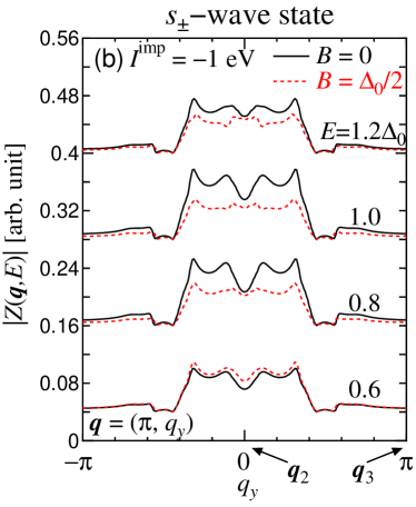
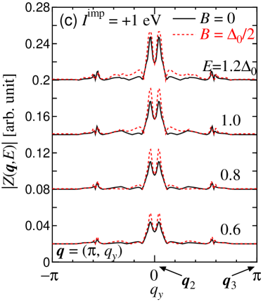
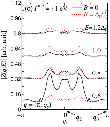
Figure 5: (Color online) Linecut from $|Z(\bm{q},E)|_{B=0}$ (solid lines) and $|Z(\bm{q},E)|_{B=\Delta_{0}/2}$ (dotted lines) maps in the isotropic two-gap case with $\Delta_{\rm h}=2\Delta_{0}$ and $\Delta_{\rm e}=\pm\Delta_{0}$ [case (ii)]. The path is shown in Fig. 4. The left and right panels show the results in the $s_{++}$-wave and $s_{\pm}$-wave states, respectively. (a),(b) $I^{\rm imp}=-1$ eV. (c),(d) $I^{\rm imp}=+1$ eV. The curves in all the figures are vertically shifted to make them visible.

Figures 5(a) and (b) show $|Z(\bm{q},E)|$ from $\bm{q}=(\pi,-\pi)$ to $(\pi,\pi)$ for $I^{\rm imp}=-1$ eV. The solid and dotted lines represent the results for $B=0$ and $\Delta_{0}/2$, respectively. For $E\sim\Delta_{0}$, the QPI peak around $\bm{q}_{2}$ is suppressed by the magnetic field in both the $s_{++}$-wave and $s_{\pm}$-wave states.

Figures 5(c) and (d) show the results for $I^{\rm imp}=+1$ eV. In the $s_{++}$-wave state, the QPI peak around $\bm{q}_{2}$ is insensitive to $B$ and $E$. On the other hand, in the $s_{\pm}$-wave state, the QPI signal shows very strong $E$ dependence, and the QPI intensity becomes very small for $E\geq 0.8\Delta_{0}$ even for $B=0$. However, such behaviors have not been observed experimentally. As results, in both the $s_{++}$-wave and $s_{\pm}$-wave states, the obtained results for $I^{\rm imp}=+1$ eV are inconsistent with experiments. Hanaguri ; Hanaguri_arxiv Therefore, impurities with weak potential will be responsible for the QPI signal in Fe(Se,Te).

In the above discussion, we have ignored the change of $T_{\rm c}$ due to the impurity scattering. We have shown that the $s_{\pm}$-wave state with the original SC transition temperature $T_{\rm c0}=30$ K is completely suppressed when the residual resistivity reaches $\sim 5z^{-1}\mu\Omega$cm, Onari_imp ; Yamakawa_imp where $z^{-1}=m^{*}/m$ is the mass-enhancement factor due to the self-energy. When $I^{\rm imp}=+1$ eV, the residual resistivity for $n^{\rm imp}=0.01$ is about $20\mu\Omega$cm in Fe-based superconductors. Therefore, the $s_{\pm}$-wave state is very fragile against impurity.

IV Discussion

IV.1 Violation of the Extinction Rule

As shown in Sec. III, the QPI peak around $\bm{q}_{2}$ is realized even in the $s_{++}$-wave state. The reason is that the numerator in Eq. (36) has finite value under the experimental condition $E<|\Delta_{\rm h,e}|$. Thus, the extinction rule in the octet model for cuprate superconductors $(|\Delta(\bm{k}_{i})|=E<\Delta^{\rm max};i=1\sim 8)$, which tells that the QPI signal at $\bm{q}=\bm{k}_{i}-\bm{k}_{j}$ disappears if $\Delta(\bm{k}_{i})=\Delta(\bm{k}_{j})$, does not hold in Fe-based superconductors under the experimental condition $E<\Delta_{0}$. As shown in Fig. 3, the QPI signal around $\bm{q}_{2}$ still exists even at $E=\Delta_{0}$ in the $s_{++}$-wave state due to the finite quasiparticle damping $\gamma$. For these reasons, we can not distinguish between the $s_{++}$-wave and $s_{\pm}$-wave states from the presence or absence of the QPI peak around $\bm{q}_{2}$.

IV.2 Comparison with Previous Studies

In Ref. Sykora, , Sykora and Coleman investigated the QPI in the $s_{\pm}$-wave state by using a two-band model. They showed that the QPI peak around $\bm{q}_{2}$ emerges for $B=0$ due to the non-magnetic impurity scattering in the weak potential limit, and its intensity is suppressed by the Zeeman effect under the magnetic field $B=\Delta_{0}$. It is consistent with the result of the present study for the weak potential case based on the five-orbital model. Also, to analyze the unitary scattering case, they phenomenologically treated the resonant scattering due to the multiple scattering process, and proposed that the QPI signal around $\bm{q}_{3}=(\pi,\pi)$ is enhanced by $B$ due to the resonant scattering. However, we cannot obtain such behavior in the present study using $T$-matrix approximation for $I^{\rm imp}=+1$ eV.

In Ref. Gao, , Gao et al. discussed the magnetic field dependence of the QPI due to the vortex, which is not considered in the present study. Interestingly, they showed that the strong and sharp QPI peak around $\bm{q}_{3}$ is caused in both the $s_{++}$-wave and $s_{\pm}$-wave states by the Andreev scattering due to the vortices. Experimentally, however, the field-induced change is almost spatially uniform, indicating that the impurity scattering is more important. Hanaguri In Ref. Gao, , the QPI peak around $\bm{q}_{2}$ was not obtained in the $s_{++}$-wave state maybe due to the very large difference in the band structure.

V Summary

In summary, we investigated the QPI in Fe-based superconductors in both the $s_{++}$-wave and $s_{\pm}$-wave states. In the octet model $\left(|\Delta(\bm{k}_{i})|=E<\Delta^{\rm max};i=1\sim 8\right)$ for cuprate superconductors with $d_{x^{2}-y^{2}}$-wave SC state, the QPI signal around $\bm{q}=\bm{k}_{i}-\bm{k}_{j}$ disappears when $\Delta(\bm{k}_{i})$ and $\Delta(\bm{k}_{j})$ have the same sign. However, this extinction rule is not hold in Fe-based superconductors with fully-gapped $s$-wave SC state. The reason is that the resonance condition, in which the denominator of the integrand in Eq. (35) becomes zero at some $\bm{k}$, does not satisfied under the experimental condition $E<|\Delta_{\rm e,h}|$. We performed the detailed numerical study of the QPI signal on the basis of the five-orbital model and found that the experimentally observed QPI peak around $\bm{q}_{2}=(\pi,0)$ can be explained in terms of both the $s_{++}$-wave and $s_{\pm}$-wave states. Furthermore, we discussed the magnetic field dependence of the QPI by considering the Zeeman effect, and found that the suppression of the peak intensity around $\bm{q}_{2}$ by the magnetic field can also be explained in terms of both the $s_{++}$-wave and $s_{\pm}$-wave states. Therefore, it is difficult to distinguish between the $s_{++}$-wave and $s_{\pm}$-wave states from the QPI experimental date for Fe-based superconductors.

Appendix A QPI in Cuprate Superconductors

In the QPI measurement for the cuprate by Hanaguri et al., Hanaguri_Cu it was shown that the QPI signals due to the impurity scattering between $\bm{k}$ points with opposite sign gap functions are strongly suppressed by the magnetic field. Since the suppression in the “matrix region” (far from vortex) is stronger than the one in the “vortex region” (near the vortex core), the Zeeman effect would be important. In this appendix, we investigate the magnetic field dependence of the QPI in cuprate superconductors with nodal $d_{x^{2}-y^{2}}$-wave SC state, $\Delta_{\bm{k}}=\Delta_{0}(\cos{k_{x}}-\cos{k_{y}})/2$, using the $T$-matrix approximation in the case of weak impurity potential $I^{\rm imp}=0.1$ eV, and show that the experimentally observed suppression can be explained by the Zeeman splitting scenario.

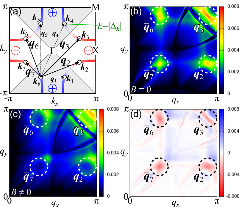
Figure 6: (Color online) (a) FS of cuprate and the $d_{x^{2}-y^{2}}$-wave SC gap. The wave vector $\bm{k}_{i}$ ($i=1\sim 8$) satisfies the relation $E=|\Delta_{\bm{k}_{i}}|$, and $\bm{q}_{i}$ is scattering vector. $\bm{q}_{2,3,6,7}$ ($\bm{q}_{1,4,5}$) connect the $\bm{k}$-points on FS with opposite (same) sign gap functions. (b) Intensity map of $|Z(\bm{q},E)|$ at $E=\Delta_{0}/2$ and $B$ = 0. The scattering vector $\bar{\bm{q}}_{i}$ is equivalent to $\bm{q}_{i}$. (c) $|Z(\bm{q},E)|$ for $B=\Delta_{0}/8$. (d) Field-induced change given by $|Z(\bm{q},E)|_{B=\Delta_{0}/8}-|Z(\bm{q},E)|_{B=0}$.

Figure 6(a) shows the FS and the gap function in cuprate superconductors. The eight wave vectors $\bm{k}_{i}$ ($i=1\sim 8$) on the FS satisfy the relation $E=|\Delta_{\bm{k}_{i}}|<\Delta_{0}$. The scattering vectors $\bm{q}_{1,4,5}$ ($\bm{q}_{2,3,6,7}$) connect the two $\bm{k}$-points with same (opposite) sign gap functions. Experimentally, the QPI signals are obtained at $\bm{q}_{2,3,6,7}$ for zero field, and they are suppressed by applying a magnetic field. Hanaguri_Cu Figure 6(b) shows the numerical results of the QPI intensity map $|Z(\bm{q},E)|_{B=0}$ without magnetic field. We use the parameters given in Ref. Maltseva, . The strong QPI peaks appear at $\bm{q}_{2,3,6,7}$. Figures 6(c) and (d) show the QPI with magnetic field, $|Z(\bm{q},E)|_{B=\Delta_{0}/8}$, and field-induced change given by $|Z(\bm{q},E)|_{B=\Delta_{0}/8}-|Z(\bm{q},E)|_{B=0}$, respectively. In this case, the QPI signal shows remarkable field dependence and its peaks at $\bm{q}_{2,3,6,7}$ are strongly suppressed by the Zeeman effect. This result is consistent with the experimental results for cuprate superconductors. Hanaguri_Cu

Appendix B QPI due to Simplified Impurity Potential

In the above discussion, we have investigated the QPI due to the orbital diagonal impurity potential in Eq. (30). In this case, the impurity potential has complex $\bm{k}$-dependence in the band basis. In this appendix, we consider the QPI due to a simple constant impurity potential in the band basis,

$$I^{\rm band}_{b,b^{\prime}}=\left\{\begin{array}[]{cc}I&(b=b^{\prime})\\ I^{\prime}&(b\neq b^{\prime})\end{array}\right.,$$ (39)

where $b=b^{\prime}$ and $b\neq b^{\prime}$ terms correspond to intraband and interband scattering, respectively. Hereafter, we study the QPI in the weak potential case with $I=I^{\prime}=0.1$ eV.

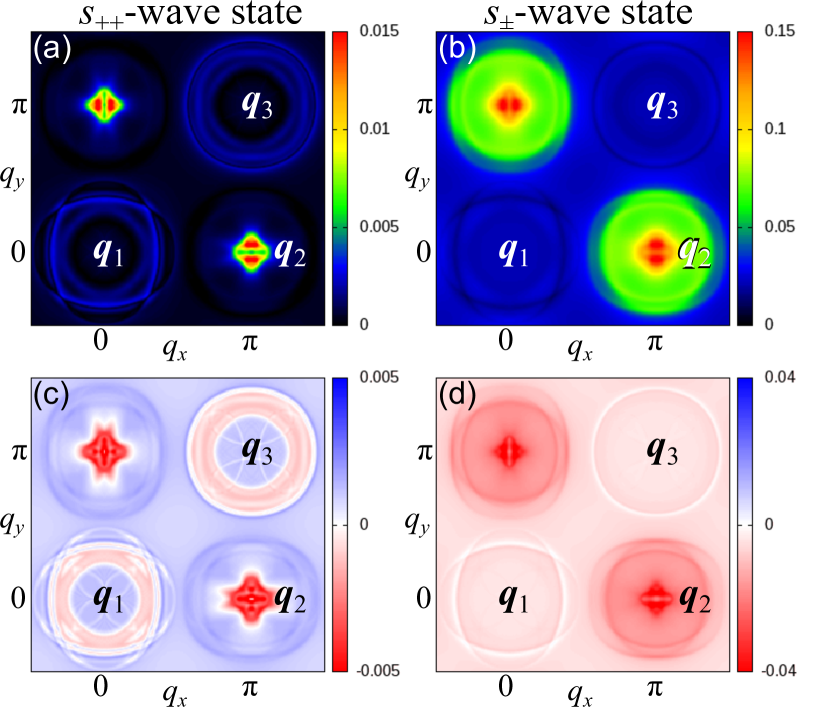
Figure 7: (Color online) (a)(b) Intensity map of the QPI $|Z(\bm{q},E)|_{B=0}$ due to the band represented weak impurity potential $I^{\rm band}_{b,b^{\prime}}=0.1$ eV in the (a) $s_{++}$-wave and (b) $s_{\pm}$-wave states. (c)(d) The magnetic field-induced change of the QPI signal given by $|Z(\bm{q},E)|_{B=\Delta_{0}/2}-|Z(\bm{q},E)|_{0}$ in the (c) $s_{++}$-wave and (d) $s_{\pm}$-wave states. We set $E=0.7\Delta_{0}$, $\Delta_{\rm h}=2\Delta_{0}$ and $\Delta_{\rm e}=\pm\Delta_{0}$.

Figures 7(a) and (b) show the QPI intensity map in the $s_{++}$-wave and $s_{\pm}$-wave states, respectively. We set $E=0.7\Delta_{0}$, $|\Delta_{\rm h}|=2\Delta_{0}$, and $|\Delta_{\rm e}|=\Delta_{0}$. The QPI peak around $\bm{q}_{2}$ appears in both the $s_{++}$-wave and $s_{\pm}$-wave states. Figures 7(c) and (d) show the field-induced change $|Z(\bm{q},E)|_{B=\Delta_{0}/2}-|Z(\bm{q},E)|_{B=0}$ in the $s_{++}$-wave and $s_{\pm}$-wave states, respectively. The obtained results are qualitatively consistent with the orbital diagonal potential case shown in Figs. 2(c), 2(d), 3(c), and 3(d) in the main text. Therefore, in the weak potential case, the obtained QPI signal is insensitive to the nature of impurity potential.

However, the impurity potential in Eq. (39) gives an erroneous result in the unitary regime $I\to\infty$, that is, the $T$-matrix $T^{\rm band}_{b,b^{\prime}}$ becomes band diagonal except for $I^{\prime}/I=1$. Due to this model artifact, the QPI peak around $\bm{q}_{2}$ disappears in the unitary limit. For the same reason, $T_{\rm c}$ in the $s_{\pm}$-wave state is almost unchanged by impurities in the unitary regime $I\rho^{0}(0)\geq 1$. Senga ; Wang However, such erroneous model artifact is revised by using a realistic potential in Eq. (30). Onari_imp ; Yamakawa_imp That is, the QPI peak around $\bm{q}_{2}$ appears and $T_{\rm c}$ in the $s_{\pm}$-wave state is fragile against impurity even in the unitary regime.

Appendix C Another Two-Gap Case with $|\Delta_{\rm h}|=1.5|\Delta_{e}|$

In the main text, we discussed the field-induced suppression of the QPI peak intensity around $\bm{q}_{2}$ in the isotropic two-gap case with $|\Delta_{\rm h}|=2|\Delta_{\rm e}|$. Here, we show another two-gap case with $|\Delta_{\rm h}|=1.5|\Delta_{\rm e}|$. The obtained results are qualitatively the same as the results for $|\Delta_{\rm h}|=2|\Delta_{\rm e}|$ in the main text.

Figure 8 shows the $|Z(\bm{q},E)|$ from $\bm{q}=(\pi,-\pi)$ to $(\pi,\pi)$ for $B=0$ (solid lines) and $B=\Delta_{0}/2$ (dotted lines). In the (a) $s_{++}$-wave and (b) $s_{\pm}$-wave states, the QPI intensity for $I^{\rm imp}=0.1$ eV around $\bm{q}_{2}$ is suppressed by $B$ for $E\sim\Delta_{0}$.

Figure 8(c) shows the $|Z(\bm{q},E)|$ in the $s_{++}$-wave state for $I^{\rm imp}=-1$ eV. In this case, the QPI intensity at just $\bm{q}_{2}$ is strongly enhanced by $B$ at $E\sim\Delta_{0}$, whereas the integrated intensity around $\bm{q}_{2}$ is suppressed. Such field-induced enhancement at just $\bm{q}_{2}$ for $E=\Delta_{0}$ is not universal since the $\bm{q}_{2}$ peak is suppressed by $B$ for $|\Delta_{\rm h}|=2|\Delta_{\rm e}|$ as shown in Fig. 5(a) in the main text. However, the obtained field-induced enhancement at just $\bm{q}_{2}$ may be consistent with the experimental result. Experimentally, the QPI signal for $E=1.0$ meV is suppressed by $B$ around $\bm{q}_{2}$, but a slight enhancement is observed at just $\bm{q}_{2}$ as shown in Fig. 1(A) in Ref. Hanaguri_arxiv, .

Figure 8 (d) shows the $|Z(\bm{q},E)|$ in the $s_{\pm}$-wave state for $I^{\rm imp}=-1$ eV. Also, Figs. 8(e) and (f) show the ones for $I^{\rm imp}=+1$ eV. In all cases (d)-(f) in Fig. 8, the obtained results are almost same as the cases (b)-(d) in Fig. 5 in the main text for $|\Delta_{\rm h}|=2|\Delta_{\rm e}|$.

Therefore, the obtained results for $|\Delta_{\rm h}|=1.5|\Delta_{\rm e}|$ are qualitatively same as the ones for $|\Delta_{\rm h}|=2|\Delta_{\rm e}|$ in the main text. The field-induced enhancement at just $\bm{q}_{2}$ for $I^{\rm imp}=-1$ eV in Fig. 8(c) may be consistent with experimental result, although it is sensitive to model parameters.

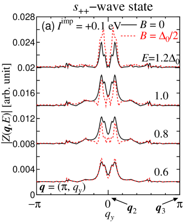
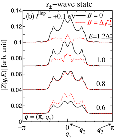
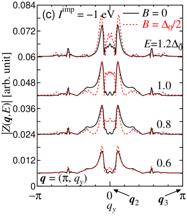
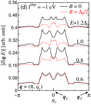
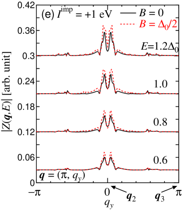
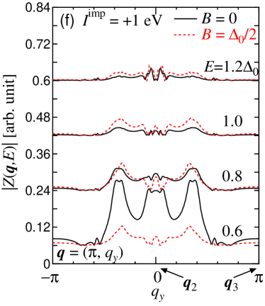
Figure 8: (Color online) $|Z(\bm{q},E)|$ along $\bm{q}=(\pi,q_{y})$ in the isotropic two-gap case with $\Delta_{\rm h}=1.5\Delta_{0}$ and $\Delta_{\rm e}=\pm\Delta_{0}$. The solid and dotted lines represent $B=0$ and $B=\Delta_{0}/2$, respectively. The left and right panels show the results in the $s_{++}$-wave and $s_{\pm}$-wave states, respectively. (a),(b) $I^{\rm imp}=0.1$ eV. (c),(d) $I^{\rm imp}=-1$ eV. (e),(f) $I^{\rm imp}=+1$ eV. The curves in all the figures are vertically shifted to make them visible.

References

- (1) Y. Kamihara, T. Watanabe, M. Hirano, and H. Hosono, J. Am. Chem. Soc. 130, 3296 (2008).
- (2) K. Kuroki, S. Onari, R. Arita, H. Usui, Y. Tanaka, H. Kontani, and H. Aoki, Phys. Rev. Lett. 101, 087004 (2008).
- (3) I. I. Mazin, D. J. Singh, M. D. Johannes, and M. H. Du, Phys. Rev. Lett. 101, 057003 (2008).
- (4) A. V. Chubukov, D. V. Efremov, and I. Eremin, Phys. Rev. B 78, 134512 (2008).
- (5) S. Graser, G. R. Boyd, C. Cao, H.-P. Cheng, P. J. Hirschfeld, and D. J. Scalapino, Phys. Rev. B 77, 180514(R) (2008).
- (6) P. J. Hirschfeld, M. M. Korshunov, and I. I. Mazin, Rep. Prog. Phys. 74, 124508 (2011).
- (7) H. Kontani and S. Onari, Phys. Rev. Lett. 104, 157001 (2010).
- (8) T. Saito, S. Onari, and H. Kontani, Phys. Rev. B 82, 144510 (2010).
- (9) S. Onari, Y. Yamakawa, and H. Kontani, Phys. Rev. Lett. 112, 187001 (2014).
- (10) M. Sato, Y. Kobayashi, S. C. Lee, H. Takahashi, E. Satomi, and Y. Miura, J. Phys. Soc. Jpn. 79, 014710 (2010).
- (11) J. Li, Y. F. Guo, S. B. Zhang, J. Yuan, Y. Tsujimoto, X. Wang, C. I. Sathish, Y. Sun, S. Yu, W. Yi, K. Yamaura, E. Takayama-Muromachiu, Y. Shirako, M. Akaogi, and H. Kontani, Phys. Rev. B 85, 214509 (2012).
- (12) Y. Nakajima, T. Taen, Y. Tsuchiya, T. Tamegai, H. Kitamura, and T. Murakami, Phys. Rev. B 82, 220504(R) (2010).
- (13) D. S. Inosov, J. T. Park, P. Bourges, D. L. Sun, Y. Sidis, A. Schneidewind, K. Hradil, D. Haug, C. T. Lin, B. Keimer, and V. Hinkov, Nat Phys 6, 178 (2010).
- (14) Y. Nakai, K. Ishida, Y. Kamihara, M. Hirano, and H. Hosono, J. Phys. Soc. Jpn. 77, 073701 (2008).
- (15) T. Hanaguri, S. Niitaka, K. Kuroki, and H. Takagi, Science 328, 474 (2010).
- (16) T. Hanaguri, S. Niitaka, K. Kuroki, and H. Takagi, arXiv:1007.0307.
- (17) S. Chi, S. Johnston, G. Levy, S. Grothe, R. Szedlak, B. Ludbrook, R. Liang, P. Dosanjh, S. A. Burke, A. Damascelli, D. A. Bonn, W. N. Hardy, and Y. Pennec, Phys. Rev. B 89, 104522 (2014).
- (18) S. Onari and H. Kontani, Phys. Rev. Lett. 103, 177001 (2009).
- (19) Y. Yamakawa, S. Onari, and H. Kontani, Phys. Rev. B 87, 195121 (2013).
- (20) S. Onari and H. Kontani, Phys. Rev. B 84, 144518 (2011). S. Onari, H. Kontani, and M. Sato, Phys. Rev. B 81, 060504(R) (2010).
- (21) Y. Yamakawa, S. Onari, and H. Kontani, Supercond. Sci. Technol. 25, 084006 (2012).
- (22) S. Sykora and P. Coleman, Phys. Rev. B 84, 054501 (2011).
- (23) Y. Gao, H. X. Huang, and P. Q. Tong, Europhys. lett. 100, 37002 (2012).
- (24) I. I. Mazin and D. J. Singh, arXiv:1007.0047.
- (25) Y.-Y. Zhang, C. Fang, X. Zhou, K. Seo, W.-F. Tsai, B. A. Bernevig, and J. Hu, Phys. Rev. B 80, 094528 (2009).
- (26) E. Plamadeala, T. Pereg-Barnea, and G. Refael, Phys. Rev. B 81, 134513 (2010).
- (27) A. Akbari, J. Knolle, I. Eremin, and R. Moessner, Phys. Rev. B 82, 224506 (2010).
- (28) T. Das and A. V. Balatsky, J. Phys.: Condens. Matter 24, 182201 (2012).
- (29) K. McElroy, R. W. Simmonds, J. E. Hoffman, D.-H. Lee, J. Orenstein, H. Eisaki, S. Uchida, and J. C. Davis, Nature 422, 592 (2003).
- (30) T. Hanaguri, Y. Kohsaka, M. Ono, M. Maltseva, P. Coleman, I. Yamada, M. Azuma, M. Takano, K. Ohishi, and H. Takagi, Science 323, 923 (2009).
- (31) M. Maltseva and P. Coleman, Phys. Rev. B 80, 144514 (2009).
- (32) M. L. Teague, G. K. Drayna, G. P. Lockhart, P. Cheng, B. Shen, H.-H. Wen, and N.-C. Yeh, Phys. Rev. Lett. 106, 087004 (2011).
- (33) M. P. Allan, A. W. Rost, A. P. Mackenzie, Y. Xie, J. C. Davis, K. Kihou, C. H. Lee, A. Iyo, H. Eisaki, and T.-M. Chuang, Science 336, 563 (2012),
- (34) T. Hānke, S. Sykora, R. Schlegel, D. Baumann, L. Harnagea, S. Wurmehl, M. Daghofer, B. Būchner, J. van den Brink, and C. Hess, Phys. Rev. Lett. 108, 127001 (2012).
- (35) P. Cai, W. Ruan, X. Zhou, C. Ye, A. Wang, X. Chen, D.-H. Lee, and Y. Wang, Phys. Rev. Lett. 112, 127001 (2014).
- (36) K. Nakamura, R. Arita, and H. Ikeda, Phys. Rev. B 83, 144512 (2011).
- (37) T. J. Williams, A. A. Aczel, E. Baggio-Saitovitch, S. L. Bud’ko, P. C. Canfield, J. P. Carlo, T. Goko, J. Munevar, N. Ni, Y. J. Uemura, W. Yu, and G. M. Luke, Phys. Rev. B 80, 094501 (2009).
- (38) K. Nakayama, T. Sato, P. Richard, Y.-M. Xu, Y. Sekiba, S. Souma, G. F. Chen, J. L. Luo, N. L. Wang, H. Ding, and T. Takahashi, Europhys. lett. 85, 67002 (2009).
- (39) Y. Ota, K. Okazaki, Y. Kotani, T. Shimojima, W. Malaeb, S. Watanabe, C.-T. Chen, K. Kihou, C. H. Lee, A. Iyo, H. Eisaki, T. Saito, H. Fukazawa, Y. Kohori, and S. Shin, Phys. Rev. B 89, 081103(R) (2014).
- (40) B. Zeng, G. Mu, H. Q. Luo, T. Xiang, I. I. Mazin, H. Yang, L. Shan, C. Ren, P. C. Dai, and H.-H. Wen, Nat Commun 1, 112 (2010).
- (41) C.-L. Song, Y.-L. Wang, P. Cheng, Y.-P. Jiang, W. Li, T. Zhang, Z. Li, K. He, L. Wang, J.-F. Jia, H.-H. Hung, C. Wu, X. Ma, X. Chen, and Q.-K. Xue, Science 332, 1410 (2011).
- (42) Y. Senga and H. Kontani, J. Phys. Soc. Jpn. 77, 113710 (2008). Y. Senga and H. Kontani, New J. Phys. 11, 035005 (2009).
- (43) Y. Wang, A. Kreisel, P. J. Hirschfeld, and V. Mishra, Phys. Rev. B 87, 094504 (2013).