Pion transverse momentum dependent parton distributions in the Nambu and Jona-Lasinio model

Abstract

An explicit evaluation of the two pion transverse momentum dependent parton distributions at leading twist is presented, in the framework of the Nambu-Jona Lasinio model with Pauli-Villars regularization. The transverse momentum dependence of the obtained distributions is generated solely by the dynamics of the model. Using these results, the so called generalized Boer-Mulders shift is studied and compared with recent lattice data. The obtained agreement is very encouraging, in particular because no additional parameter has been introduced. A more conclusive comparison would require a precise knowledge of the QCD evolution of the transverse momentum dependent parton distributions under scrutiny.
KEYWORDS: Deep Inelastic Scattering, Phenomenological Models, Chiral Lagrangians

1 Introduction

The three-dimensional (3D) hadronic structure in momentum space can be accessed through the transverse momentum dependent parton distributions (TMDs) [1], measured mainly in semi-inclusive deep inelastic scattering (SIDIS) or in Drell-Yan (DY) processes. For the nucleon target a large amount of theoretical work is being done, driven by recent and forthcoming impressive experimental efforts (see, e.g, [2, 3, 4] and references therein). In this paper we discuss pion TMDs, which are experimentally probed through the DY process (see, e.g., [5] for a recent report).

At leading-twist, the pion structure is described in terms of two TMDs, the unpolarized one, $f_{1,\pi}(x,k^{2}_{T})$, describing the number density of partons with longitudinal momentum fraction $x$ and transverse momentum $k_{T}$, and the Boer-Mulders TMD, also called Boer-Mulders function, $h_{1,\pi}^{\perp}(x,k^{2}_{T})$ [6, 7]. The latter is not a density, being generated by spin-orbit correlations of transversely polarized partons; it is chiral-odd and therefore not accessible in DIS, and it is “naively” time-reversal odd, i.e., under time reversal the correlation flips the sign.

TMDs are non perturbative quantities and they have not been calculated from first principles, although recently lattice data have been produced for the pion. In particular, the lattice calculation in Ref. [8], performed at the pion mass $m_{\pi}=518$ MeV, is the update of preliminary results reported in [9, 10]. Pion TMDs have been estimated also in models of the pion structure, such as spectator models [11, 12, 13], bag models [14], covariant model of the pion with Pauli-Villars regulators, in the unpolarized case [15], and in a light-front constituent quark model [16].

In this paper we present the calculation of $f_{1,\pi}(x,{k}^{2}_{T})$ and $h_{1,\pi}^{\perp}(x,{k}^{2}_{T})$ in the model of Nambu and Jona-Lasinio (NJL) [17].

The NJL model is the most realistic model for the pseudoscalar mesons based on a local quantum field theory built with quarks. It respects the realization of chiral symmetry and gives a good description of low energy properties. Mesons are described as bound states, in a fully covariant way, using the Bethe-Salpeter amplitude, in a field theoretical framework. In this way, the Lorentz covariance of the problem is preserved. The NJL model is a non-renormalizable field theory and therefore a cut-off procedure has to be implemented. Here, the Pauli-Villars regularization scheme has been chosen, because it respects the gauge symmetry of the problem. The NJL model, together with its regularization procedure, can be regarded as an effective theory of QCD.

The NJL model has a long tradition of successful predictions of different observables related to the parton structure of pseudoscalar mesons, such as the parton distribution [18, 19], generalized parton distributions [20], distribution amplitudes [21], transition distribution amplitudes [22, 23], transition form factors [24, 25, 26]. Here, for the first time, we apply the same scheme to the calculation of the pion TMDs. This will permit to obtain a dynamical $k_{T}$ dependence, at variance with various other model analyses where its analytical trend was assumed, and to compare it with very recent lattice data [8].

The paper is structured as follows. In Section 2 we describe our approach obtaining the formal results. In the third Section we discuss the numerical results and, at the end, we perform the comparison with lattice data. Conclusions are eventually presented in the last section.

2 TMDs in the NJL model

For a spinless particle, such as the pion, only two leading twist TMDs arise, in contrast to the eight found for spin-$\frac{1}{2}$ particles [3]. The TMD $f_{1,\pi}$ is simply the unpolarized quark distribution, whereas the Boer-Mulders (BM) function [6], $h_{1,\pi}^{\perp}$, describes the distribution of transversely polarized quarks in the pion. The BM function is odd under time reversal (T-odd). A non-zero value for this function is originated by the final and initial state interactions, in the SIDIS and DY processes, respectively, which break the symmetry of the events under time reversal.

The calculation of $f_{1,\pi}$ and $h_{1,\pi}^{\perp}$ in the NJL model will be described in the following two subsections, respectively.

2.1 Unpolarized TMD

The unpolarized quark TMD in the pion is defined as follows

$$f_{1,\pi}^{u(d)}\left(x,k_{T}^{2}\right) = \frac{1}{2}\int\frac{d\xi^{-}\,d^{2}\xi_{T}}{\left(2\pi\right)^{3}}\,e^{-i\left(\xi^{-}\,k^{+}-\vec{\xi}_{T}\vec{k}_{T}\right)}$$ (1)

$$\times \left\langle p\right|\bar{\psi}\left(\xi^{-},\vec{\xi}_{T}\right)\,\mathcal{L}_{\vec{\xi}_{T}}^{\dagger}\left(\infty,\xi^{-}\right)\,\gamma^{+}\,\frac{1}{2}\left(1\pm c\tau_{3}\right)\,\mathcal{L}_{0}\left(\infty,0\right)\,\psi\left(0\right)\left|p\right\rangle~{},$$

where $c=1(-1)$ stands for the $u(d)$ case, $k^{+}=xP^{+}$, $\xi^{+}=0,$ and the gauge link is given by

$$\mathcal{L}_{\vec{\xi}_{T}}\left(\infty,\xi^{-}\right)=\mathcal{P}\,\exp\left(-ig_{s}\int_{\xi^{-}}^{\infty}A^{+}\left(\eta^{-},\vec{\xi}_{T}\right)\,d\eta^{-}\right)~{},$$ (2)

with $g_{s}$ the strong $SU\left(3\right)_{c}$ coupling constant.

To fix the ideas, we consider the $u$ quark TMD in a $\pi^{+}.$ At zero order in $g_{s}$, one gets

$$f_{1,\pi}\left(x,k_{T}^{2}\right)=\frac{1}{2}\int\frac{d\xi^{-}\,d^{2}\xi_{T}}{\left(2\pi\right)^{3}}\,e^{-i\left(\xi^{-}\,k^{+}-\vec{\xi}_{T}\vec{k}_{T}\right)}\,\left\langle p\right|\bar{\psi}\left(\xi^{-},\vec{\xi}_{T}\right)\,\gamma^{+}\,\frac{1}{2}\left(1+\tau_{3}\right)\,\psi\left(0\right)\left|p\right\rangle~{}.$$ (3)

The two diagrams contributing to this quantity are shown in Fig. 1. The contribution of the diagram in the left panel is

$$f_{1,\pi}\left(x,k_{T}^{2}\right) =-\frac{1}{2}\int\frac{d^{4}q}{\left(2\pi\right)^{4}}\delta\left(k^{+}-\frac{P^{+}}{2}-q^{+}\right)\,\delta^{2}\left(k_{T}-\frac{P_{T}}{2}-q_{T}\right)$$

$$\times\mathrm{Tr}\left(iS_{F}\left(q-\frac{P}{2}\right)\,ig_{\pi qq}\,\,i\gamma_{5}\,\tau_{-}\,iS_{F}\left(q+\frac{P}{2}\right)\right.$$

$$\times\left.\gamma^{+}\,iS_{F}\left(q+\frac{P}{2}\right)\,ig_{\pi qq}\,\,i\gamma_{5}\,\tau_{+}\right)~{},$$ (4)

where Tr implies traces in color, flavor and Dirac matrices, $S_{F}(p)$ is the Feynman propagator and $\tau_{\pm}={1\over\sqrt{2}}(\tau_{1}\pm i\tau_{2})$. The other diagram of Fig. 1, corresponding to the propagation of a $\sigma$ particle, which gives sometimes important contributions (see for instance the calculation of pion GPDs in [20]), vanishes in this case, where a diagonal matrix element of a bi-local current is involved.

Figure 1: The diagrams to be considered in the evaluation of the $u$ TMD in a $\pi^{+}$, Eq. (3).

After Pauli Villars regularization (see the Appendix for details), the final result is

$$f_{1,\pi}\left(x,k_{T}^{2}\right) =\frac{3}{4\,\pi^{3}}\,g_{\pi qq}^{2}\,\theta\left(x\right)\,\theta\left(1-x\right)\,\sum_{i=0}^{2}c_{i}$$

$$\times\,\left\{\frac{1}{k_{T}^{2}+M_{i}^{2}-m_{\pi}^{2}\,x\left(1-x\right)}+\frac{m_{\pi}^{2}\,x\left(1-x\right)}{\left[k_{T}^{2}+M_{i}^{2}-m_{\pi}^{2}\,x\left(1-x\right)\right]^{2}}\right\}~{}.$$ (5)

The integration over $k_{T}^{2}$ of the TMD yields the pion PD

$$q\left(x\right) =\int d^{2}k_{T}\,f_{1,\pi}\left(x,k_{T}^{2}\right)$$

$$=\int\frac{d\xi^{-}}{2\pi}\,e^{-i\xi^{-}\,k^{+}}\left\langle p\right|\bar{\psi}\left(\xi^{-}\right)\,\mathcal{L}_{0}^{\dagger}\left(\infty,\xi^{-}\right)\,\gamma^{+}\,\mathcal{L}_{0}\left(\infty,0\right)\,\psi\left(0\right)\left|p\right\rangle~{},$$ (6)

with $k^{+}=xP^{+}$, $\xi^{+}=0$ and $\vec{\xi}_{T}=\vec{0}.$ One gets explicitly

$$q\left(x\right) = \frac{3}{4\pi^{2}}\,g_{\pi qq}^{2}\,\theta\left(x\right)\,\theta\left(1-x\right)$$ (7)

$$\times \sum_{i=0}^{2}c_{i}\,\left\{\ln\frac{m^{2}-m_{\pi}^{2}\,x\left(1-x\right)}{\left(M_{i}^{2}-m_{\pi}^{2}\,x\left(1-x\right)\right)}+\frac{m_{\pi}^{2}\,x\left(1-x\right)}{\left[M_{i}^{2}-m_{\pi}^{2}\,x\left(1-x\right)\right]}\right\}~{}.$$

We stress that, since we are working in a field theoretical scheme, the right support of the distributions, $0\leq x\leq 1$, is not imposed and arises naturally. For the same reason, one can easily proof that: i) the normalization is correct, i.e., $\int dx~{}q\left(x\right)=1$; ii) $\int dx~{}x~{}q\left(x\right)=0.5$, i.e., the fraction of momentum carried by each quark is one half of the total momentum. Since at this level there are no sea quarks, this is the expected correct result.

2.2 Boer-Mulders function

The BM function is defined as

$$h_{1,\pi}^{\perp\,u(d)}\left(x,k_{T}^{2}\right) = \epsilon^{i\,j\,}k_{T}^{j}\,\frac{m_{\pi}}{2\,k_{T}^{2}}\int\frac{d\xi^{-}\,d^{2}\xi_{T}}{\left(2\pi\right)^{3}}\,e^{-i\left(\xi^{-}\,k^{+}-\vec{\xi}_{T}\vec{k}_{T}\right)}$$

$$\times \left\langle p\right|\bar{\psi}\left(\xi^{-},\vec{\xi}_{T}\right)\,\mathcal{L}_{\vec{\xi}_{T}}^{\dagger}\left(\infty,\xi^{-}\right)\,i\,\sigma^{i\,+}\,\gamma_{5}\,\frac{1}{2}\left(1\pm c\,\tau_{3}\right)\,\mathcal{L}_{0}\left(\infty,0\right)\,\psi\left(0\right)\left|p\right\rangle~{},$$

with the same conventions used in Eq. (1). To fix the ideas, as previously done for the unpolarized TMD, we will consider the BM function for a $u$ quark in a $\pi^{+}$.

At zero order in $g_{s}$, $h_{1,\pi}^{\perp}$ vanishes, due to the T-odd character of the BM function. In order to have a non-zero value of the BM function, we expand the gauge link $\mathcal{L}_{\vec{\xi}_{T}}\left(\infty,\xi^{-}\right)$, Eq. (2) in powers of $g_{s}$, up to the first order, as it has been done for phenomenological model estimates of T-odd parton distributions, for the nucleon (see, e.g., Refs. [27, 28, 29, 30, 31]) and, recently, for the pion [16]. For the gluonic field, we use its definition in terms of the source

$$A^{a\,+}\left(\eta\right)=\int d^{4}y~{}D^{+\,\nu}\left(\eta-y\right)\,g_{s}\,\bar{\psi}\left(y\right)\,\frac{\lambda^{a}}{2}\,\gamma_{\nu}\,\psi\left(y\right)~{},$$ (9)

where $D^{\mu\,\nu}\left(x-y\right)$ is the gluon propagator. After some calculation, we arrive at

$$\mathcal{L}_{\vec{\xi}_{T}}\left(\infty,\xi^{-}\right) \simeq 1-g_{s}^{2}\,\frac{\lambda^{a}}{2}\int\frac{d^{4}t}{\left(2\pi\right)^{4}}e^{i\,\vec{t}_{T}\vec{\xi}_{T}}\ e^{-i\,t^{+}\xi^{-}}~{}\frac{1}{t^{+}-i\varepsilon}\$$ (10)

$$\times \frac{-1}{t^{2}+i\varepsilon}\int d^{4}y~{}e^{i\,t\,y}\,\bar{\psi}\left(y\right)\,\frac{\lambda^{a}}{2}\,\gamma^{+}\,\psi\left(y\right)~{}.$$

At the first order in $g_{s}^{2}$ one gets

$$h_{1,\pi}^{\perp}\left(x,k_{T}^{2}\right) = \epsilon^{i\,j\,}k_{T}^{j}\,\frac{m_{\pi}}{2\,k_{T}^{2}}\,g_{s}^{2}\int\frac{d\xi^{-}\,d^{2}\xi_{T}}{\left(2\pi\right)^{3}}\,e^{-i\left(\xi^{-}\,k^{+}-\vec{\xi}_{T}\vec{k}_{T}\right)}\left\langle p\right|\bar{\psi}\left(\xi^{-},\vec{\xi}_{T}\right)$$

$$\times \,\left\{\frac{\lambda^{a}}{2}\int\frac{d^{4}t}{\left(2\pi\right)^{4}}e^{i\,\vec{t}_{T}\vec{\xi}_{T}}\ e^{-i\,t^{+}\xi^{-}}~{}\frac{1}{t^{+}-i\varepsilon}\ \frac{-1}{t^{2}+i\varepsilon}\right.$$

$$\times \left.\int d^{4}y~{}e^{i\,t\,y}\,\bar{\psi}\left(y\right)\,\frac{\lambda^{a}}{2}\,\gamma^{+}\,\psi\left(y\right)\,i\,\sigma^{i\,+}\,\gamma_{5}\,\right.$$

$$- i\,\sigma^{i\,+}\,\gamma_{5}\,\left.\frac{\lambda^{a}}{2}\int\frac{d^{4}t}{\left(2\pi\right)^{4}}~{}\frac{1}{t^{+}-i\varepsilon}\ \frac{-1}{t^{2}+i\varepsilon}\int d^{4}y~{}e^{i\,t\,y}\,\bar{\psi}\left(y\right)\,\frac{\lambda^{a}}{2}\,\gamma^{+}\,\psi\left(y\right)\right\}\,\psi\left(0\right)\left|p\right\rangle~{}~{}.$$

A straightforward calculation leads to

$$h_{1,\pi}^{\perp}\left(x,k_{T}^{2}\right) = -\epsilon^{i\,j\,}k_{T}^{j}\,\frac{m_{\pi}}{2\,k_{T}^{2}}\,g_{s}^{2}\,g_{\pi qq}^{2}\,\int\frac{d^{4}t\,~{}dr^{-}}{\left(2\pi\right)^{8}}\,\frac{1}{t^{+}-i\varepsilon}\,\frac{1}{t^{2}+i\varepsilon}$$ (12)

$$\times \left\{-\mathrm{Tr}\left[S_{F}\left({\small r+t-}\tfrac{P}{2}\right)\gamma_{5}\,\tau_{-}\,S_{F}\left({\small r+t+}\tfrac{P}{2}\right)\tfrac{\lambda^{a}}{2}i\sigma^{i\,+}\gamma_{5}\right.\right.$$

$$\times \left.\left.S_{F}\left({\small r+}\tfrac{P}{2}\right)\gamma_{5}\,\tau_{+}S_{F}\left({\small r-}\tfrac{P}{2}\right)\tfrac{\lambda^{a}}{2}\gamma^{+}\right]\right.$$

$$+ \left.\mathrm{Tr}\left[S_{F}\left({\small r-}\tfrac{P}{2}\right)\gamma_{5}\,\tau_{-}\,S_{F}\left({\small r+}\tfrac{P}{2}\right)\tfrac{\lambda^{a}}{2}i\sigma^{i\,+}\gamma_{5}\right.\right.$$

$$\times \left.\left.S_{F}\left({\small r-t+}\tfrac{P}{2}\right)\gamma_{5}\,\tau_{+}S_{F}\left({\small r-t-}\tfrac{P}{2}\right)\tfrac{\lambda^{a}}{2}\gamma^{+}\right]\right\}~{},$$

where $r=\left(\left(x-\frac{1}{2}\right)P^{+},\vec{k}_{T},r^{-}\right).$ The traces in the equation above, in the order they appear, correspond to the diagrams in the left and right panels of Fig. 2, respectively. In principle, the BM function could have contributions also from the sigma term (the one reported in Fig. 1, right panel, in the unpolarized case). The direct calculation shows anyway that these contributions vanish.

Figure 2: The diagrams describing the two traces in Eq. (12).

After a lengthy calculation, and including the Pauli Villars renormalization, we obtain

$$h_{1,\pi}^{\perp}\left(x,k_{T}^{2}\right) = -\frac{1}{\sqrt{2}\,\pi^{3}}\,\frac{m\,m_{\pi}}{k_{T}^{2}}\,\alpha_{s}\,g_{\pi qq}^{2}\,\theta\left(x\right)\,\theta\left(1-x\right)\,\sum_{i=0}^{2}c_{i}\,\frac{1}{k_{T}^{2}+M_{i}^{2}-m_{\pi}^{2}\,x\left(1-x\right)}$$ (13)

$$\times \ln\left[\frac{k_{T}^{2}+M_{i}^{2}-m_{\pi}^{2}\,x\left(1-x\right)}{M_{i}^{2}-m_{\pi}^{2}\,x\left(1-x\right)}\right]~{},$$

where we have introduced the strong coupling constant $\alpha_{s}={g_{s}^{2}\over 4\pi}$.

The $k_{T}$ integral can be calculated, providing

$$h_{\pi}(x) = \int d^{2}k_{T}\,h_{1,\pi}^{\perp}\left(x,k_{T}^{2}\right)=-\frac{1}{6\,\sqrt{2}}\,m\,m_{\pi}\,\alpha_{s}\,g_{\pi qq}^{2}\,\theta\left(x\right)\,\theta\left(1-x\right)$$ (14)

$$\times \,\sum_{i=0}^{2}c_{i}\,\frac{1}{M_{i}^{2}-m_{\pi}^{2}\,x\left(1-x\right)}~{},$$

which, integrated over $x$, yields

$$\int dx\int d^{2}k_{T}\,h_{1,\pi}^{\perp}\left(x,k_{T}^{2}\right)=-\frac{1}{6\,\sqrt{2}}\,m\,\alpha_{s}\,g_{\pi qq}^{2}\,\sum_{i=0}^{2}c_{i}\,\frac{4\operatorname{arccsc}\left(2\frac{M_{i}}{m_{\pi}}\right)}{\sqrt{\left(4\,M_{i}^{2}-m_{\pi}^{2}\right)}}~{}.$$ (15)

In the $m_{\pi}\rightarrow 0$ limit, we get

$$\lim_{m_{\pi}\rightarrow 0}\int dx\int d^{2}k_{T}\,h_{1,\pi}^{\perp}\left(x,k_{T}^{2}\right)=-\frac{1}{6\,\sqrt{2}}\,m_{\pi}\,m\,\alpha_{s}\,g_{\pi qq}^{2}\,\sum_{i=0}^{2}\frac{c_{i}}{M_{i}^{2}}~{}.$$ (16)

At variance with the $f_{1,\pi}(x,k_{T}^{2})$ case, in which $\int dx\,dk_{T}^{2}\,f_{1,\pi}(x,k_{T}^{2})=1$ is a consequence of charge conservation, the quantity (16) is not in general related to any physical observable. However we note that, in the present NJL framework and in the chiral limit, one has $g_{\pi qq}^{2}\,\sum_{i=0}^{2}\frac{c_{i}}{M_{i}^{2}}={4\over 3}\pi^{2}r_{\pi}^{2}$, i.e., the right hand side of Eq. (16) can be related to $r_{\pi}$, the charge radius of the pion.

3 Discussion and comparison with lattice data

3.1 Unpolarized TMD

To have a pictorial representation of the global $x$ and $k_{T}$ dependencies, 3D-plots are shown in Fig. 3, for $m_{\pi}=$ 140 MeV (left panel) and $m_{\pi}=518$ MeV (right panel). In the left panel,

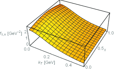
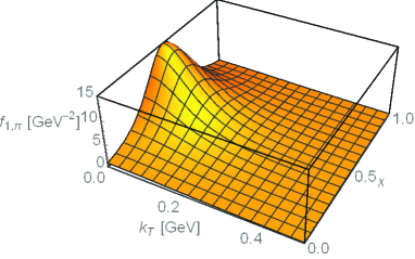
Figure 3: The unpolarized TMD $f_{1,\pi}\left(x,k_{T}^{2}\right)$, as a function of $k_{T}$ and $x$, with $m_{\pi}=140$ MeV (left panel) and $m_{\pi}=518$ MeV (right panel).

it can be seen that the unpolarized TMD varies slowly with $x$. This is easily understood looking at Eq. (5), where $x$ dependent terms always appear multiplied by $m_{\pi}^{2}$. In the right panel of Fig. 3 it is clearly seen that, by taking a heavy pion with $m_{\pi}$ = 518 MeV, a value which will be useful later for the comparison with lattice data, the $x$ dependence becomes much more pronounced. In the latter situation, our results agree qualitatively with the findings of Ref. [15, 16], where different constituent quark models have been used to evaluate the unpolarized TMDs. This fact can be understood thinking that, in the present NJL approach, the chiral limit is naturally included, at variance with a constituent quark scenario, where chiral symmetry is explicitly broken. As a consequence, the $x$ dependence of our results with a pion mass of $m_{\pi}=$ 518 MeV is closer to that obtained within constituent quark models, with respect to what is obtained in our approach using the physical pion mass.

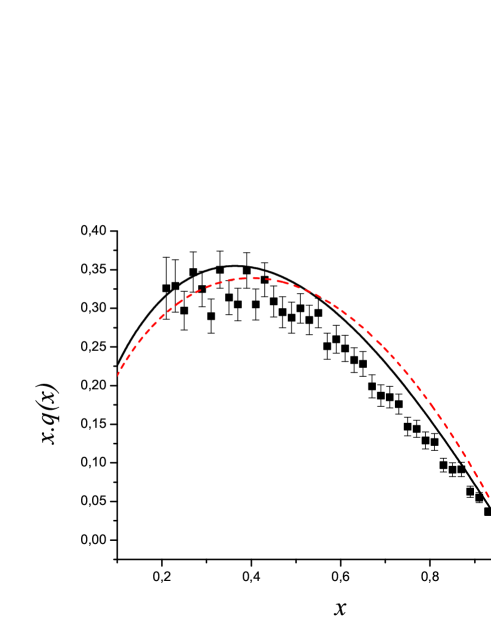
Figure 4: The pion PD, Eq. (7), after LO (solid line) and NLO (dashed line) QCD evolution to $Q=2$ GeV (picture taken from Ref. [23]). Data are from Ref. [34].

The rather flat $x$ dependence, obtained using $m_{\pi}=140$ MeV, is not a drawback of the model. Hadron models, like the NJL model, must be regarded as a realization of QCD at a very low $Q^{2}$. Evolution will change the $x$ dependence in an important way. In fact, starting from Eq (7), in Refs. [32] and [23, 33], a very good description of the data of the pion parton distribution at $Q=2$ GeV [34] is obtained, as one can see in Fig. 4, taken from [23]. For later convenience, it is useful to report that the LO parameters of the QCD evolution used in Refs. [32] and [23, 33] predict $\alpha_{s}($2 GeV$)$ = 0.32 and $\alpha_{s}($2 GeV$)$ = 0.29, respectively. These values are in good agreement with $\alpha_{s}$ measured in correspondence of the mass of the $\tau$ lepton, $\alpha_{s}(m_{\tau}=1.777$ GeV$)=0.327^{+0.019}_{-0.016}$ [35].

Concerning the relation between mass and $x$ dependence, it is also interesting to observe that, in the chiral limit, the NJL model predicts an absolutely flat parton distribution, $q_{\chi}(x)=1$, and distribution amplitude, $\phi_{\chi}(x)=1$. Nevertheless, the different regime of evolution (DGLAP for the first quantity and ERBL for the second one) produces very different $x$ dependencies at higher $Q^{2}$ [24].

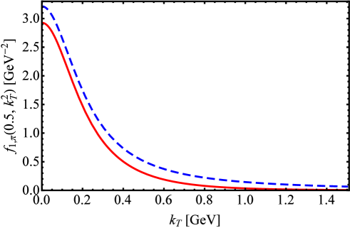
Figure 5: The unpolarized TMD $f_{1,\pi}\left(x,k_{T}^{2}\right)$, Eq. (5), at $x=0.5$, for the physical pion, as a function of $k_{T}$ (full). The dashed curve does not include the counter terms coming from the regularization procedure.

In Fig. 5, the $k_{T}$ dependence is shown, having fixed $x=0.5$. The result without the contributions of the counter terms originated by the regularization procedure is also reported. It is worth stressing that, in our approach, the $k_{T}$ dependence is automatically generated by the NJL dynamics. This is an important feature of our results, not found in other approaches. In facts, for example, the two different $k_{T}$ dependencies of the unpolarized TMD shown in Ref. [15] are dictated by two different forms adopted for a regulator function appearing in the pion Bethe-Salpeter amplitude. In a similar fashion, in the Light-Front scenario of Ref. [16], the obtained $k_{T}$-dependence is determined by the gaussian form assumed in the pion light-cone wave function, following Refs. [36, 37]. In our case, the $k_{T}$ dependence is not imposed using an educated guess. It is therefore relevant to report that our prediction has the following asymptotic $k_{T}$ behavior, as it can be obtained from Eq. (5):

$$f_{1,\pi}\left(x,k_{T}^{2}\right)\xrightarrow[k_{T}^{2}\to\infty]{}\frac{3g_{\pi qq}^{2}\Lambda^{4}}{2\pi^{3}k_{T}^{6}}~{}.$$ (17)

We reiterate that this is just a consequence of the NJL model with Pauli-Villars regularization. To this respect, Fig. 5 points out the importance of the regularization procedure. In facts, without the counter terms, which suppress the high $k_{T}$ region, the TMD would not be integrable in the variable $k_{T}^{2}$. Actually, as it has been shown above, the integration over $k_{T}^{2}$ of the TMD yields the pion PD.

3.2 Boer-Mulders function

Numerical results of the evaluation of the BM function, Eq. (13), divided by the strong coupling constant, are reported in Fig. 6, in a 3D-plot, providing a pictorial representation of the global $x$ and $k_{T}$ dependencies.

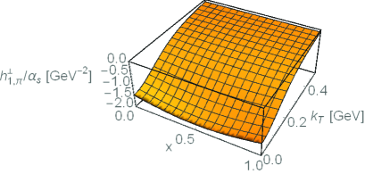
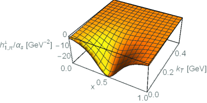
Figure 6: The Boer-Mulders TMD, $h_{1,\pi}^{\perp}\left(x,k_{T}^{2}\right)$, divided by the strong coupling constant $\alpha_{s}$, evaluated using $m_{\pi}=140$ MeV (left panel) and $m_{\pi}=518$ MeV (right panel).

As it happens for the unpolarized TMD, the BM TMD varies slowly with $x$ when the physical pion mass, $m_{\pi}$ = 140 MeV, is used in our calculation. This is again easily understood looking at Eq. (13), where $x$ dependent parts always appear multiplied by $m_{\pi}^{2}$. In the right panel of Fig. 6, it is shown that, by taking $m_{\pi}$ = 518 MeV, the $x$ dependence becomes much more relevant.

As for the unpolarized TMD, the obtained $k_{T}$ behavior is a genuine result of the NJL dynamics with Pauli-Villars regularization. We report our prediction for the asymptotic $k_{T}$ behavior of the BM TMD, as it can be obtained from Eq. (13):

$$h_{1,\pi}^{\perp}\left(x,k_{T}^{2}\right) \xrightarrow[k_{T}^{2}\to\infty]{} \theta(x)\theta(1-x)\,\frac{mm_{\pi}\alpha_{s}g_{\pi qq}^{2}}{\sqrt{2}\pi^{3}k_{T}^{4}}\,\sum_{i=0}^{2}\,c_{i}\,log{M_{i}^{2}-m_{\pi}^{2}x(1-x)\over m^{2}-m_{\pi}^{2}x(1-x)}$$ (18)

$$+ O\left({1\over k_{T}^{6}}log(k_{T})\right)$$

3.3 Comparison with lattice data

In the following, we compare our results with lattice measurements. In facts, very recently, a lattice calculation has been performed [8], focused on a TMD observable related to the Boer-Mulders effect in a pion.

The quantity which has been addressed is a ratio, defined in an appropriate way to be safely evaluated on the lattice. It is the so called “generalized Boer-Mulders shift”, given by the following expression

$$\langle k_{y}\rangle_{UT}(b_{T}^{2})\equiv m_{\pi}\frac{\tilde{h}_{1}^{\perp[1](1)}(b_{T}^{2})}{\tilde{f}_{1}^{[1](0)}(b_{T}^{2})}~{},$$ (19)

where ${\tilde{h}_{1}^{\perp[1](1)}(b_{T}^{2})}$ and ${\tilde{f}_{1}^{[1](0)}(b_{T}^{2})}$ are $x$-moments of generic Fourier-transformed TMDs:

$$\tilde{f}^{[m](n)}(b_{T}^{2}) = n!\left(-\frac{2}{m_{\pi}^{2}}\partial_{b_{T}^{2}}\right)^{n}\int_{-1}^{1}dx\,x^{m-1}\int d^{2}k_{T}\,e^{ib_{T}\cdot k_{T}}\ f(x,k_{T}^{2})$$

$$= \frac{2\pi n!}{(m_{\pi}^{2})^{n}}\,\int_{-1}^{1}dx\,x^{m-1}\int d|k_{T}|\,|k_{T}|\,\left(\frac{|k_{T}|}{|b_{T}|}\right)^{n}J_{n}(|b_{T}||k_{T}|)f(x,k_{T}^{2})~{},$$

with $J_{n}$ denoting the Bessel functions of the first kind.

One should notice that the $b_{T}\rightarrow 0$ limit of the generalized Boer-Mulders shift, Eq. (19), formally corresponds to $k_{T}^{2}$-moments of TMDs,

$$\tilde{f}^{[m](n)}(0) = \int_{-1}^{1}dx\,x^{m-1}\int d^{2}k_{T}\ \left(\frac{k_{T}^{2}}{2m_{\pi}^{2}}\right)^{n}\ f(x,k_{T}^{2})$$ (21)

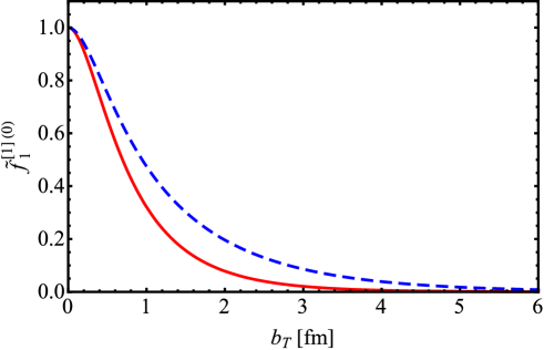
Figure 7: The moment ${\tilde{f}_{1}^{[1](0)}(b_{T}^{2})}$ of the unpolarized pion TMD, calculated assuming the physical pion mass, $m_{\pi}=140$ MeV (full line), or $m_{\pi}=518$ MeV, the value used in the lattice calculation in Ref. [8] (dashed line).

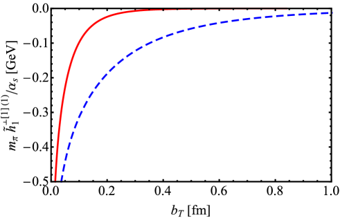
Figure 8: The same as in Fig. 7, for $m_{\pi}$ times the moment $\tilde{h}_{1}^{\perp[1](1)}(b_{T}^{2})$ of the Boer-Mulders pion TMD, divided by $\alpha_{s}$.

In the $b_{T}\rightarrow 0$ limit, the generalized Boer-Mulders shift reduces therefore to the “Boer-Mulders shift”,

$$\langle k_{y}\rangle_{UT}(0)=m_{\pi}\frac{\tilde{h}_{1}^{\perp[1](1)}(0)}{\tilde{f}_{1}^{[1](0)}(0)}~{},$$ (22)

which has the meaning of the average transverse momentum in $y$-direction of quarks polarized in the transverse (“$T$”) $x$-direction, in an unpolarized (“$U$”) pion, normalized to the corresponding number of valence quarks.

It should be noted, however, that the $k_{T}^{2}$-moments of TMDs (21) appearing in (22) are in general divergent at large $k_{T}$ and thus not well-defined without an additional regularization. In the generalized quantity, (19), a finite $b_{T}$ effectively acts as a regulator through the associated Bessel weighting, cf. (3.3). For these reasons, in Ref. [8], lattice QCD data have been obtained for the generalized Boer-Mulders shift (19), at finite $b_{T}$, using a pion mass of 518 MeV.

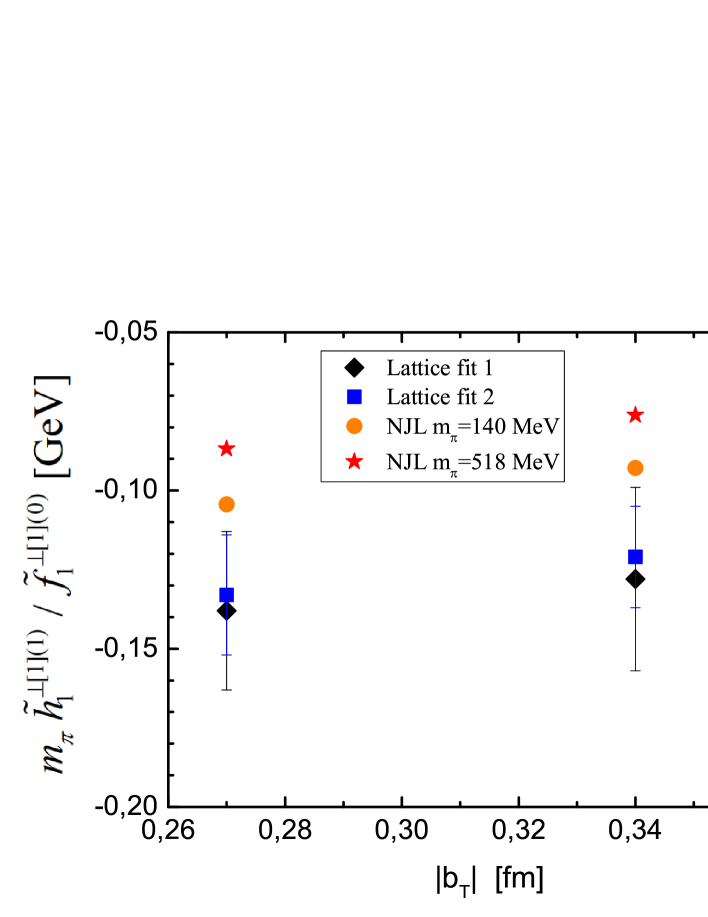
Figure 9: The generalized Boer-Mulders shift, Eq. (19), as a function of $b_{T}$. The orange circles are obtained using the present NJL approach with $m_{\pi}=140$ MeV; the red stars are obtained using $m_{\pi}=518$ MeV, the value at which the lattice measurement has been performed. Two different sets of lattice data (black and blue boxes), with their RMS deviation, obtained in Ref. [8] using independent fits, are shown for comparison.

In the following, we compare these lattice results with the outcome of our approach. The numerator and denominator of the generalized BM shift, Eq. (19), i.e., the moments ${\tilde{f}_{1}^{[1](0)}(b_{T}^{2})}$ and $m_{\pi}\tilde{h}_{1}^{\perp[1](1)}(b_{T}^{2})$, are shown in Figs. 7 and 8, respectively, as a function of $b_{T}$, for $m_{\pi}=140$ MeV (full line) and $m_{\pi}=518$ MeV (dashed line). In Fig. 7 we observe that, by increasing the pion mass, ${\tilde{f}_{1}^{[1](0)}(b_{T}^{2})}$ is shifted towards higher values of $b_{T}$. This is consistent with the fact that the e.m. radius of the pion is smaller for $m_{\pi}=140$ MeV than for $m_{\pi}=518$ MeV (see the Appendix for the actual values). In Fig. 8 we compensated an overall factor $m_{\pi}^{-1}$ present in $\tilde{h}_{1}^{\perp[1](1)}(b_{T}^{2})$ multiplying the latter quantity by the corresponding pion mass. We observe the same behavior, in relation with the variation of the mass, as in Fig. 7. Nevertheless, it is difficult to give any simple intuitive explanation because here we are dealing with a two body operator, as it can be seen from Fig. 2 or Eq. (2.2).

In Ref. [8], lattice data for the generalized Boer-Mulders shift have been presented for three different values of $b_{T}$, at the momentum scale $Q=2$ GeV, given in [38]. Our model results have therefore to be evolved to this scale, for a proper comparison with the lattice calculation. Unfortunately, the complete QCD evolution of the moments ${\tilde{f}_{1}^{[1](0)}(b_{T}^{2})}$ and $h_{1}^{\perp[1](1)}(b_{T}^{2})$, involving both the $x$ and $k_{T}$ dependencies, is not under control. In particular, the evolution of the $k_{T}$ dependence is basically unknown. To estimate the evolution of the $x$ dependence of the denominator, we can approximate it with the behavior of the corresponding $k_{T}$ integrated quantity, the first moment of the PD, which does not evolve in $x$. For the numerator, being $h_{1}^{\perp[1](1)}(b_{T}^{2})$ proportional to $\alpha_{s}(Q^{2})$ through the BM function, for a first estimate one can assume that its evolution is basically governed by that of $\alpha_{s}(Q^{2})$. It is therefore important to fix properly the value of $\alpha_{s}$ in evaluating the model prediction for the generalized Boer-Mulders shift at 2 GeV. Following the discussion on the fixing of the LO evolution parameters in NJL calculations of parton distributions, reported in the previous section, we use $\alpha_{s}$ = 0.31.

$\left|b_{T}\right|$	Lattice 1	Lattice 2	NJL$~{}m_{\pi}=140$ MeV	NJL$~{}m_{\pi}=518$ MeV
fm	GeV	GeV	GeV	GeV
0.27	-0.138(28)	-0.133(19)	-0.104	-0.087
0.34	-0.128(29)	-0.121(16)	-0.093	-0.076
0.36	-0.145(25)	-0.148(15)	-0.090	-0.074

Table 1: The generalized Boer-Mulders shift, Eq. (19), as a function of $b_{T}$. The first column corresponds to the three values of $b_{T}$ analyzed in Ref. [8]. The second and third columns contain the two different sets of lattice data, with their RMS deviation, obtained in Ref. [8] using independent fits. In the fourth and fifth columns the results obtained using the present NJL approach are given, with $m_{\pi}=140$ MeV and $m_{\pi}=518$ MeV, the value at which the lattice measurement has been performed.

In Fig. 9 and Tab. 1 our results are compared with the lattice data, evaluated according to two different fits providing consistent results [6]. We obtain a reasonably good agreement. It must be emphasized that our calculation has been performed in the NJL model without introducing any new parameter. We observe that the generalized Boer-Mulders shift varies slowly when we go from $m_{\pi}=140$ MeV to $m_{\pi}=518$ MeV.

The main uncertainty in our calculation comes from the poorly known QCD evolution of the moments of the TMDs, entering the definition of the generalized Boer-Mulders shift. Summarizing our approximated evolution scheme, the $x$ evolution of the denominator has been neglected thinking to the behavior of the corresponding PD, the one of the numerator has been assumed to be governed by that of $\alpha_{s}$ only, and the $k_{T}$ evolution has been neglected overall.

4 Conclusions

We have considered the well-established NJL model, without any additional parameter, for the study of the two leading twist pion TMDs, the unpolarized, $f_{1,\pi}(x,k_{T}^{2})$, and the Boer-Mulders one, $h_{1,\pi}^{\perp}(x,k_{T}^{2})$. We were motivated by the success of this model in reproducing pion observables, such as the parton distribution and the pion gamma transition form factor, and by the aim of reproducing recent lattice results [8]. Since in the latter calculation a value of 518 MeV has been used for the pion mass, we present our results for $m_{\pi}=140$ MeV and $m_{\pi}=518$ MeV.

We have studied the $k_{T}$ dependence of $f_{1,\pi}(x,k_{T}^{2})$ and $h_{1,\pi}^{\perp}(x,k_{T}^{2})$. In both cases, this dependence is automatically generated by the NJL dynamics. The obtained $k_{T}$ asymptotic behavior of these two quantities, at the momentum scale of the model, $Q_{0}$, is found to be $k_{T}^{-6}$ and $k_{T}^{-4}$, respectively. Nevertheless, QCD evolution to higher scales could modify these trends.

We observe a soft dependence on $x$ in both TMDs at $Q_{0}$. This can be easily understood observing that, in the final expressions of the TMDs, the $x$-dependent part is always multiplied by $m_{\pi}$. Our experience with the parton distribution and the distribution amplitude of the pion is that this $x$ dependence provides remarkably good results after QCD evolution. When the $m_{\pi}=518$ MeV case is considered, we get a stronger $x$ dependence, approaching results obtained in models built with constituent quarks.

Finally, we have studied the generalized Boer-Mulders shift, which has been recently calculated. The agreement we obtain with these lattice data is rather good, qualitatively and quantitatively. Our results show a weak dependence on the mass of the pion.

The main theoretical uncertainty in our calculation comes from the approximated QCD evolution we have performed. A more conclusive comparison would require therefore further lattice data and the implementation of the correct evolution of the TMDs moments appearing in the calculation.

5 Acknowledgments

This work was supported in part by the Mineco under contract FPA2013-47443-C2-1-P, by GVA-Prometeo/II/2014/066, by CPAN(CSD- 00042) and by the Centro de Excelencia Severo Ochoa Programme grant SEV-2014-0398. S.S. thanks the Department of Theoretical Physics of the University of Valencia for warm hospitality and support. S.N. thanks the INFN, sezione di Perugia, the University of Perugia and the Department of Physics and Geology of the University of Perugia for warm hospitality and support.

Appendix A The NJL model and regularization scheme

The Lagrangian density in the two-flavor version of the NJL model with electromagnetic (e.m.) coupling is

$$\mathcal{L}=\bar{\psi}\left(i\,\not D-m_{0}\right)\psi+g\left[\left(\bar{\psi}\,\psi\right)^{2}+\left(\bar{\psi}\,\vec{\tau}\,i\gamma_{5}\,\psi\right)^{2}\right]$$

with $D_{\mu}=\partial_{\mu}+i\,e\,A_{\mu}.$

The NJL model is a non-renormalizable field theory and a cut-off procedure must be defined. We have used the Pauli-Villars regularization in order to render the occurring integrals finite. This means that, for any integral, we make the replacement

$$\int\frac{d^{4}q}{\left(2\pi\right)^{4}}f\left(q;m\right)~{}\longrightarrow~{}\int\frac{d^{4}q}{\left(2\pi\right)^{4}}\,\sum_{j=0}^{2}\,c_{j}\,f\left(q;M_{j}\right)$$

with $M_{j}^{2}=m^{2}+j\,\Lambda^{2}$, $c_{0}=c_{2}=1$ and $c_{1}=-2$. Following ref. [17] we determine the regularization parameter $\Lambda$ and $m$ by calculating the pion decay constant and the quark condensate in the chiral limit, via

$$f_{\pi}^{2}=-\frac{3\,m^{2}}{4\,\pi^{2}}\sum_{j=0}^{2}\,c_{j}\,\log\frac{M_{j}^{2}}{m^{2}}~{},~{}~{}~{}\ \ \ \ \ \ \ \ ~{}\left\langle\bar{u}u\right\rangle=-\frac{3\,m}{4\,\pi^{2}}\sum_{j=0}^{2}\,c_{j}\,M_{j}^{2}\,\log\frac{M_{j}^{2}}{m^{2}}$$

with $m_{0}$ fixing the pion mass.

With the conventional values $\left\langle\bar{u}u\right\rangle=-(0.250\operatorname{GeV})^{3},$ $f_{\pi}=0.0924\operatorname{GeV}$ and $m_{\pi}=0.140\operatorname{GeV}$, we get $m=0.238\operatorname{GeV}$, $\Lambda=0.860\operatorname{GeV}$ and $m_{0}=5.4\operatorname{MeV}.$ For the pion-quarks coupling constant we get $g_{\pi qq}^{2}=6.279$. The electromagnetic pion radius turns out to be $r_{\pi}^{2}=0.31\operatorname{fm}^{2}$ (experimental value $r_{\pi}^{2}=0.44\operatorname{fm}^{2}$).

For a proper comparison with lattice data, we have applied the same model to a massive pion, with $m_{\pi}=0.518\operatorname{GeV}.$ We have not changed the value of $\Lambda$; for $m$ we have taken $m=0.300\operatorname{GeV}.$ In this way we have $\left\langle\bar{u}u\right\rangle=-(0.263\operatorname{GeV})^{3},$ $f_{\pi}=0.0997\operatorname{GeV}$, $m_{0}=83$ MeV and $g_{\pi qq}^{2}=3.667.$ The e.m. pion radius is $r_{\pi}^{2}=0.38\operatorname{fm}^{2}.$

References

- [1] J. C. Collins and D. E. Soper, “Parton Distribution and Decay Functions,” Nucl. Phys. B 194, 445 (1982).
- [2] A. Bacchetta, M. Diehl, K. Goeke, A. Metz, P. J. Mulders and M. Schlegel, “Semi-inclusive deep inelastic scattering at small transverse momentum,” JHEP 0702 (2007) 093 [hep-ph/0611265].
- [3] V. Barone, F. Bradamante and A. Martin, “Transverse-spin and transverse-momentum effects in high-energy processes,” Prog. Part. Nucl. Phys. 65 (2010) 267. [arXiv:1011.0909 [hep-ph]].
- [4] R. Angeles-Martinez et al., “Transverse momentum dependent (TMD) parton distribution functions: status and prospects,” arXiv:1507.05267 [hep-ph].
- [5] J.-C. Peng and J.-W. Qiu, “Novel Phenomenology of Parton Distributions from the Drell-Yan Process,” Prog. Part. Nucl. Phys. 76, 43 (2014). [arXiv:1401.0934 [hep-ph]].
- [6] D. Boer and P. J. Mulders, “Time-reversal odd distribution functions in leptoproduction,” Phys. Rev. D 57, 5780 (1998). [arXiv:hep-ph/9711485].
- [7] D. Boer, “Investigating the origins of transverse spin asymmetries at RHIC,” Phys. Rev. D 60, 014012 (1999). [arXiv:hep-ph/9902255].
- [8] M. Engelhardt, P. Hägler, B. Musch, J. Negele and A. Schäfer, “Lattice QCD study of the Boer-Mulders effect in a pion,” arXiv:1506.07826 [hep-lat].
- [9] M. Engelhardt, B. Musch, P. Hägler, J. Negele and A. Schäfer, “Lattice study of the Boer-Mulders transverse momentum distribution in the pion,” arXiv:1310.8335 [hep-lat].
- [10] B. U. Musch, P. Hägler, M. Engelhardt, J. W. Negele and A. Schäfer, “Sivers and Boer-Mulders observables from lattice QCD,” Phys. Rev. D 85, 094510 (2012). [arXiv:1111.4249 [hep-lat]].
- [11] Z. Lu and B.-Q. Ma, “Non-zero transversity distribution of the pion in a quark-spectator-antiquark model,” Phys. Rev. D 70, 094044 (2004). [hep-ph/0411043].
- [12] M. Burkardt and B. Hannafious, “Are all Boer-Mulders functions alike?,” Phys. Lett. B 658, 130 (2008) [arXiv:0705.1573 [hep-ph]].
- [13] L. Gamberg and M. Schlegel, “Final state interactions and the transverse structure of the pion using non-perturbative eikonal methods,” Phys. Lett. B 685, 95 (2010). [arXiv:0911.1964 [hep-ph]].
- [14] Z. Lu, B.-Q. Ma and J. Zhu, “Boer-Mulders function of the pion in the MIT bag model,” Phys. Rev. D 86, 094023 (2012) [arXiv:1211.1745 [hep-ph]].
- [15] T. Frederico, E. Pace, B. Pasquini and G. Salmè, “Pion Generalized Parton Distributions with covariant and Light-front constituent quark models,” Phys. Rev. D 80 (2009) 054021 [arXiv:0907.5566 [hep-ph]].
- [16] B. Pasquini and P. Schweitzer, “Pion transverse momentum dependent parton distributions in a light-front constituent approach, and the Boer-Mulders effect in the pion-induced Drell-Yan process,” Phys. Rev. D 90 (2014) 1, 014050. [arXiv:1406.2056 [hep-ph]].
- [17] S. P. Klevansky, “The Nambu-Jona-Lasinio model of quantum chromodynamics,” Rev. Mod. Phys. 64 (1992) 649.
- [18] R. M. Davidson and E. Ruiz Arriola, “Structure Functions Of Pseudoscalar Mesons In The SU(3) Njl Model” Phys. Lett. B 348 (1995) 163.
- [19] R. M. Davidson, E. Ruiz Arriola, “Parton distributions functions of pion, kaon and eta pseudoscalar mesons in the NJL model,” Acta Phys. Polon. B33, 1791-1808 (2002). [hep-ph/0110291].
- [20] L. Theussl, S. Noguera and V. Vento, “Generalized parton distributions of the pion in a Bethe-Salpeter approach,” Eur. Phys. J. A 20 (2004) 483 [arXiv:nucl-th/0211036].
- [21] E. Ruiz Arriola and W. Broniowski, “Pion light-cone wave function and pion distribution amplitude in the Nambu-Jona-Lasinio model,” Phys. Rev. D 66 (2002) 094016 [arXiv:hep-ph/0207266].
- [22] A. Courtoy and S. Noguera, “The Pion-Photon Transition Distribution Amplitudes in the Nambu-Jona Lasinio Model,” Phys. Rev. D 76 (2007) 094026 [arXiv:0707.3366 [hep-ph]].
- [23] A. Courtoy, Ph. D. Thesis, Valencia University, 2009. http://arxiv.org/abs/arXiv:1010.2974
- [24] S. Noguera and V. Vento, “The pion transition form factor and the pion distribution amplitude,” Eur. Phys. J. A 46, 197 (2010) [arXiv:1001.3075 [hep-ph]].
- [25] S. Noguera and S. Scopetta, “The eta-photon transition form factor,” Phys. Rev. D 85, 054004 (2012) [arXiv:1110.6402 [hep-ph]].
- [26] S. Noguera and V. Vento, “Model analysis of the world data on the pion transition form factor,” Eur. Phys. J. A 48 (2012) 143 [arXiv:1205.4598 [hep-ph]].
- [27] S. J. Brodsky, D. S. Hwang and I. Schmidt, “Final state interactions and single spin asymmetries in semiinclusive deep inelastic scattering,” Phys. Lett. B 530 (2002) 99 [hep-ph/0201296].
- [28] A. Courtoy, F. Fratini, S. Scopetta and V. Vento, “A Quark model analysis of the Sivers function,” Phys. Rev. D 78 (2008) 034002 [arXiv:0801.4347 [hep-ph]].
- [29] A. Courtoy, S. Scopetta and V. Vento, “Model calculations of the Sivers function satisfying the Burkardt Sum Rule,” Phys. Rev. D 79, 074001 (2009) [arXiv:0811.1191 [hep-ph]].
- [30] A. Courtoy, S. Scopetta and V. Vento, “Analyzing the Boer-Mulders function within different quark models,” Phys. Rev. D 80 (2009) 074032 [arXiv:0909.1404 [hep-ph]].
- [31] B. Pasquini and F. Yuan, “Sivers and Boer-Mulders functions in Light-Cone Quark Models,” Phys. Rev. D 81, 114013 (2010) [arXiv:1001.5398 [hep-ph]].
- [32] W. Broniowski, E. Ruiz Arriola and K. Golec-Biernat, “Generalized parton distributions of the pion in chiral quark models and their QCD evolution,” Phys. Rev. D 77 (2008) 034023 [arXiv:0712.1012 [hep-ph]].
- [33] A. Courtoy and S. Noguera, “Enhancement effects in exclusive pi pi and rho pi production in gamma* gamma scattering,” Phys. Lett. B 675 (2009) 38 [arXiv:0811.0550 [hep-ph]].
- [34] J. S. Conway et al., “Experimental Study of Muon Pairs Produced by 252-GeV Pions on Tungsten,” Phys. Rev. D 39, 92 (1989).
- [35] K. A. Olive et al. [Particle Data Group Collaboration], “Review of Particle Physics,” Chin. Phys. C 38 (2014) 090001.
- [36] F. Schlumpf, “Charge form-factors of pseudoscalar mesons,” Phys. Rev. D 50, 6895 (1994). [hep-ph/9406267].
- [37] P. L. Chung, F. Coester and W. N. Polyzou, “Charge Form-Factors of Quark Model Pions,” Phys. Lett. B 205, 545 (1988).
- [38] B. U. Musch, P. Hagler, J. W. Negele and A. Schafer, “Exploring quark transverse momentum distributions with lattice QCD,” Phys. Rev. D 83 (2011) 094507 [arXiv:1011.1213 [hep-lat]].