The Bohmian Approach to the Problems of Cosmological Quantum Fluctuations

Abstract

There are two kinds of quantum fluctuations relevant to cosmology that we focus on in this article: those that form the seeds for structure formation in the early universe and those giving rise to Boltzmann brains in the late universe. First, structure formation requires slight inhomogeneities in the density of matter in the early universe, which then get amplified by the effect of gravity, leading to clumping of matter into stars and galaxies. According to inflation theory, quantum fluctuations form the seeds of these inhomogeneities. However, these quantum fluctuations are described by a quantum state which is homogeneous and isotropic, and this raises a problem, connected to the foundations of quantum theory, as the unitary evolution alone cannot break the symmetry of the quantum state. Second, Boltzmann brains are random agglomerates of particles that, by extreme coincidence, form functioning brains. Unlikely as these coincidences are, they seem to be predicted to occur in a quantum universe as vacuum fluctuations if the universe continues to exist for an infinite (or just very long) time, in fact to occur over and over, even forming the majority of all brains in the history of the universe. We provide a brief introduction to the Bohmian version of quantum theory and explain why in this version, Boltzmann brains, an undesirable kind of fluctuation, do not occur (or at least not often), while inhomogeneous seeds for structure formation, a desirable kind of fluctuation, do.

1 Introduction

The notion of observation or measurement plays a fundamental role in standard quantum theory. One of the basic postulates of quantum mechanics is namely that upon measurement the Schrödinger evolution of the wave function is interrupted by a collapse. However, the notions of observer or measurement are rather vague. Exactly which physical processes count as measurements? What counts as an observer? All living creatures? Or only humans? Or only humans with a Ph.D.? And why should there be special rules for measurement in quantum mechanics to begin with, without which there would apparently be no collapses—and no results of measurements? This is one version of the measurement problem of quantum mechanics.

This problem is especially severe in the context of cosmology. How can we describe the early universe when there were no measurements or observers? An adequate description requires what Bell [1, 2] dubbed a quantum theory without observers, a theory in which observers or measurements do not play a fundamental role. One such theory is Bohmian mechanics [3, 4]. Bohmian mechanics describes a configuration of particles and/or fields and/or metrics, or in general some kind of variables associated with space-time points, called local be-ables (as opposed to observ-ables), which evolve under the influence of the wave function. In Bohmian mechanics it is the local beables and their behavior, not measurement or observation, that is fundamental.

In this paper we want to consider two problems in quantum cosmology which are closely related to the quantum measurement problem and explain how they get resolved in the context of Bohmian mechanics. These problems have to do with vacuum fluctuations. On the one hand, according to current cosmological theories, all structure (i.e., non-uniformity of matter, such as stars and galaxies) is supposed to come out of vacuum fluctuations. The problem, emphasized particularly by Sudarsky and collaborators [5, 6, 7], is how these quantum fluctuations can turn into classical perturbations of the matter density. The other problem, emphasized by Boddy, Carroll, and Polack [8, 9], has to do with vacuum fluctuations at late times. At late times, it is expected that the universe will be driven to homogeneity due to the continuing expansion of the universe, driven by the cosmological constant. All that remains are vacuum fluctuations. These vacuum fluctuations are believed to yield every possible configuration over time, in particular “Boltzmann brains” which, if the universe continues to exist long enough, will outnumber the ordinary brains. According to the “Copernican principle” [10], which states that we should expect not to occupy a privileged position in the universe, we should expect to be one of the Boltzmann brains. But our observations show clearly that we are not Boltzmann brains, which puts our cosmological theory into question.

The outline of the paper is as follows. The problems of cosmological quantum fluctuations are described in more detail in section 2. In section 3, we provide an introduction to Bohmian mechanics and explain the basic mechanisms with which the Bohmian approach can address these problems. In section 4, we describe a concrete Bohmian model of quantum field theory on a curved background space-time with an expanding Friedman-Lemaître-Robertson-Walker metric, in terms of which we analyze the problem of Boltzmann brains and, in section 5, the problem of classical perturbations from quantum fluctuations.

2 Problems of vacuum fluctuations in cosmology

According to current cosmological models, our universe is believed to spatially expand exponentially fast both at early and late times. According to inflation theory, which describes the early times, the inflaton field is driving the expansion. At late times, the cosmological constant is causing the expansion. In both cases, the expansion drives the universe to homogeneity, so that nothing remains but vacuum fluctuations. These vacuum fluctuations are regarded as a virtue in the early universe, but as a vice in the late universe. In the early universe they are considered to be the seeds of structure formation, while in the late universe they lead to the problem of Boltzmann brains.

2.1 Problem with seeds of structure formation

To illustrate the nature of the difficulty, it may be helpful to consider the following simple example. As a toy model, consider non-relativistic, Newtonian gravity for $N$ point particles in a large box $\Lambda=[0,L]^{3}$ with periodic boundary conditions. According to classical mechanics, if this system starts out in a near-uniform configuration (with initial velocities, say, equal to zero, or random with a Gaussian distribution), it evolves to a clumped configuration under the influence of gravity; that is, gravity will amplify any slight initial non-uniformity. Now in quantum mechanics, consider a constant wave function $\psi_{0}$ on configuration space $\Lambda^{N}$; it gives $>99\%$ weight to near-uniform configurations and evolves, under the Schrödinger equation over a suitable duration $t$, to a wave function $\psi_{t}$ that gives $>99\%$ weight to clumped configurations but is still invariant under 3-translations because $\psi_{0}$ and the Hamiltonian are. So $\psi_{t}$ has a symmetry that the clumped configuration we observe does not have. That is, $\psi_{t}$ is a superposition of many “clumped states,” and not a random clumped state, and $\psi_{t}$ contains no information about which clumped configuration is the real one. This problem is, of course, a variant of the usual measurement problem of quantum mechanics, but it is exacerbated in cosmology, where we cannot exploit what an observer outside the system would see upon a measurement.

The same kind of problem arises in current cosmological theories, such as inflation theory. The formation of structure such as stars and galaxies requires initial perturbations in the matter density. According to inflation theory, the vacuum fluctuations of the metric field and inflaton field are the seeds for these matter density perturbations. During the inflationary expansion, the inflaton and metric fields are approximately homogeneous and isotropic. The deviations from homogeneity and isotropy are described by the vacuum state which, however, is itself homogeneous and isotropic as a quantum state. This inflationary period lasts until the inflaton field decays into ordinary matter fields. It is believed that during the inflationary period these quantum vacuum fluctuations became classical field perturbations. Once the inflaton field decays into ordinary matter, the matter distribution inherits the non-homogeneity of these perturbations. The inhomogeneities in the matter density then grow because of gravitational clumping, to eventually form large scale structures such as stars, galaxies and clusters of galaxies. An imprint of these fluctuations at the time of decoupling (when the photons were allowed to move freely) can be found in the temperature pattern of the micro-wave background radiation. The precise details of these temperature fluctuations allows us to distinguish between different inflationary models.

This is regarded as part of the success story of inflation theory [11, 12, 13, 14, 15]. However, there is still a problem with the standard presentation. Namely, how exactly did the vacuum fluctuations, which are described by a quantum state that is homogeneous and isotropic, give rise to classical field perturbations that no longer have this symmetry? After all, the unitary evolution preserves the symmetry. Hence, according to standard quantum theory, the symmetry can only be broken by collapse of the wave function. But collapse of the wave function is supposed to happen upon measurement. What physical process is playing the role of a measurement in the early universe? There are no measurement devices or observers around at that time. Moreover, objects such as measurement devices or observers (which are obviously inhomogeneous) are themselves supposed to stem, ultimately, from the quantum fluctuations in the metric and inflaton fields.

In order to address this problem, one needs a precise version of quantum mechanics, which does not suffer from the measurement problem. One class of precise approaches is collapse theories, where collapses happen spontaneously at random times, according to an observer-independent law. An analysis of the problem at hand in the context of collapse theories has been carried out by a number of people, especially by Sudarsky and collaborators [5, 16, 17, 6, 18, 19, 7]. An analysis in terms of Bohmian mechanics has also been carried out [20, 21]. We will turn to it in sections 3.3 and 5.

2.2 Problem with Boltzmann brains

In addition, at late times, there is the worry of Boltzmann brains [22, 23, 24, 25, 8, 9].

We begin by explaining what a Boltzmann brain is. Let $M$ be the present macro-state of your brain. For a classical gas in thermal equilibrium, after sufficient waiting time some atoms will, with probability 1, “by coincidence” (or “by fluctuation”) happen to come together in such a way as to form a subsystem in a micro-state compatible with $M$ (at least if the classical dynamics is “sufficiently ergodic,” which we shall assume here). That is, this brain comes into existence not by fetal development and, prior to that, evolution of life forms, but by coincidence; this brain has memories (duplicates of your present memories), but they are false memories: the events described in the memories never happened to this brain. Boltzmann brains are, of course, very unlikely. But they will form if the waiting time is long enough, and they will form more frequently if the system is larger (larger volume and number of particles).

Let us explain why Boltzmann brains can lead to a problem. According to the “Copernican principle” [10], we should be typical observers in a typical universe. This principle can be understood as a rule for extracting predictions from a theory: we should see what a typical observer (weighted with life span) in a typical universe sees. For example, consider classical mechanics with the additional constraint that the initial micro-state of the universe is compatible with a certain low-entropy macro-state; in a typical solution of the dynamical equations (“typical universe”), entropy increases with time, so, according to the Copernican principle, the theory predicts that we should see entropy increase; this is, in fact, Boltzmann’s explanation of the observed entropy increase.

Now the following problem with Boltzmann brains arises. Imagine for example a classical non-relativistic universe in a finite volume. Suppose that the universe continues to exist forever, so that the whole universe reaches thermal equilibrium at some time in the distant future. After an extremely long waiting time, a Boltzmann brain will spontaneously form out of some particles in the thermal equilibrium; since the universe exists forever, this unlikely event is certain to happen sooner or later. After a short while the Boltzmann brain will disintegrate, and the universe will again be in thermal equilibrium. After another extremely long waiting time, the next Boltzmann brain will form, probably in another place and from other particles. If time is infinite, this is again certain to happen. And to happen again and again. In fact, the number of times this will happen is by far greater than the total number of brains that ever grew as part of the evolution of life before the universe reached global thermal equilibrium. Thus, the overwhelming majority of brains in the universe will be Boltzmann brains. According to the Copernican principle, the theory predicts that we are Boltzmann brains. But we are not. After all, as emphasized by Feynman [26, p. 115], most fluctuations leading to Boltzmann brains will be no larger than necessary, so Boltzmann brains find themselves surrounded by thermal equilibrium, not by other living beings on a tepid planet orbiting a hot star. So, the theory makes a wrong prediction. The question is how any of our serious theories can avoid making this wrong prediction.

Here is a concrete version of the problem. As emphasized by Boddy, Carroll, and Polack [8, 9], there is reason to believe that the late universe will be close to de Sitter space-time (e.g., this occurs in the $\Lambda$CDM model), that all matter will be driven to homogeneity, and that the quantum state that describes the deviations from uniformity will locally look like the Bunch-Davies vacuum, a quantum state that is invariant under all isometries of de Sitter space-time. For the sake of definiteness, let us take for granted in the following that the late universe is approximately de Sitter, at least in large regions, although the discussion of the problem does not depend much on that. On any kind of configuration space (be it of particle or field configurations), the probability distribution that the Bunch-Davies vacuum defines gives positive probability to all sorts of configurations, including Boltzmann brain configurations. Does this mean there are Boltzmann brains sparsely scattered around in the Bunch-Davies vacuum? Or, could Boltzmann brains occur, rarely but over and over during an infinite amount of time, in the Bunch-Davies vacuum?

This leads to the question, What is the significance of this particular wave function for reality? Does a stationary state mean that nothing happens? Carroll adheres to the many-worlds view of quantum mechanics, and he and other advocates of many-worlds (such as David Wallace [27]) disagree about whether a stationary state means that nothing happens. If it means that nothing happens, this would remove the problem, as we discuss in section 3.5 below. While the many-worlds view seems ambiguous about this question, the Bohmian approach naturally provides an unambiguous answer: in any given Bohm-type model, it is clear whether Boltzmann brains do or do not occur. We will argue in sections 3.5 and 4.3 that in natural models, they do not occur.

3 Bohmian mechanics

We now describe non-relativistic Bohmian mechanics (also called pilot-wave theory or de Broglie-Bohm theory), a theory about point particles in physical space moving under the influence of the wave function. Later in section 4, we describe an extension of this theory for a field in curved space-time.

3.1 Definition of the theory

The equation of motion for the configuration $X=({\bf X}_{1},\dots,{\bf X}_{n})$ of the particle positions reads

$${\dot{X}}(t)=v^{\psi}(X(t),t)$$ (1)

where the velocity vector field $v^{\psi}=({\bf v}^{\psi}_{1},\dots,{\bf v}^{\psi}_{n})$ is given by

$${\bf v}^{\psi}_{k}=\frac{1}{m}{\textrm{Im}}\left(\frac{\psi^{*}\boldsymbol{\nabla}_{k}\psi}{\psi^{*}\psi}\right)\,.$$ (2)

For particles without spin this assumes the form

$${\bf v}^{\psi}_{k}=\frac{1}{m}{\textrm{Im}}\left(\frac{\boldsymbol{\nabla}_{k}\psi}{\psi}\right)=\frac{1}{m}\boldsymbol{\nabla}_{k}S\,,\qquad\psi=|\psi|\mathrm{e}^{\mathrm{i}S}\,.$$ (3)

The wave function $\psi(x,t)=\psi({\bf x}_{1},\dots,{\bf x}_{n},t)$ itself satisfies the non-relativistic Schrödinger equation

$$\mathrm{i}\partial_{t}\psi(x,t)=\left(-\sum^{n}_{k=1}\frac{1}{2m_{k}}\boldsymbol{\nabla}^{2}_{k}+V(x)\right)\psi(x,t)\,.$$ (4)

Examples of Bohmian trajectories are shown in Figure 1 for a single particle in a double-slit setup.

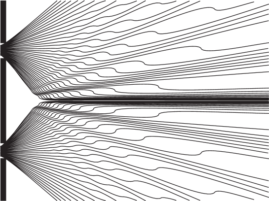
Figure 1: Several alternative possible Bohmian trajectories of a particle passing through a double-slit setup with the wave function passing through both slits. The selection of trajectories shown follows roughly the $|\psi|^{2}$ distribution. Picture created by G. Bauer after [28].

For an ensemble of systems all with the same wave function $\psi$, there is a distinguished distribution given by $|\psi|^{2}$, which is called the quantum equilibrium distribution. This distribution is equivariant: it is preserved by the particles dynamics (1) in the sense that if the particle distribution is given by $|\psi(x,t_{0})|^{2}$ at some time $t_{0}$, then it is given by $|\psi(x,t)|^{2}$ at all times $t$. This follows from the facts that any distribution $\rho$ that is transported by the particle motion satisfies the continuity equation

$$\partial_{t}\rho+\sum^{n}_{k=1}\boldsymbol{\nabla}_{k}\cdot(\rho{\bf v}^{\psi}_{k})=0$$ (5)

and that $|\psi|^{2}$ satisfies the same equation, i.e.,

$$\partial_{t}|\psi|^{2}+\sum^{n}_{k=1}\boldsymbol{\nabla}_{k}\cdot(|\psi|^{2}{\bf v}^{\psi}_{k})=0$$ (6)

as a consequence of the Schrödinger equation (4).

We note that, as a consequence of the equation of motion (1) with (2) or (3), if the wave function factorizes, as in

$$\psi({\bf x}_{1},\ldots,{\bf x}_{n})=\varphi({\bf x}_{1},\ldots,{\bf x}_{m})\,\chi({\bf x}_{m+1},\ldots,{\bf x}_{n})\,,$$ (7)

then the subsystem ${\bf X}_{1},\ldots,{\bf X}_{m}$ obeys the analogous equation of motion involving only $\varphi$, as $\chi$ cancels out.

In Bohmian mechanics, it is meaningful to speak of the wave function of the universe because, in the Bohmian approach, the wave function is not primarily regarded as a tool for predicting what observers will see but as a part of the physical world. In particular, Equations (1)–(4) define a simple, non-relativistic model of the universe with $n$ particles, with $\psi$ the wave function of the universe. Assuming (as we will henceforth) that the initial configuration of the universe $X(t=0)$ is typical with respect to the $|\psi(x,0)|^{2}$ distribution (i.e., as if randomly chosen with $|\psi(x,0)|^{2}$ distribution), it can be shown [29, 30, 31] that the empirical predictions of Bohmian mechanics agree with the standard quantum formalism.

Note that the velocity vector field is of the form $v^{\psi}=j^{\psi}/|\psi|^{2}$, where $j^{\psi}=({\bf j}^{\psi}_{1},\dots,{\bf j}^{\psi}_{n})$ with ${\bf j}^{\psi}_{k}={\textrm{Im}}(\psi^{*}\boldsymbol{\nabla}_{k}\psi)/m$ is the usual quantum-mechanical probability current. In other quantum theories, such as for example quantum field theories, the equation of motion can be set up in a similar way by dividing the appropriate current by the density. In this way it is ensured that the dynamics will leave the density equivariant. (See for example [32] for a treatment of arbitrary Hamiltonians.)

In a Bohmian universe, there is the wave function $\psi$ of the universe and a configuration $Q$ of the universe describing the arrangement of all fundamental fields and particles. There is also a natural definition for the wave function $\varphi$ of a subsystem with configuration $X$—corresponding to a splitting $Q=(X,Y)$ of the configuration of the universe into that of the subsystem and that of its environment, $Y$—called the conditional wave function. For example in the context of non-relativistic quantum mechanics, the conditional wave function of a subsystem is given by $\varphi(x,t)=\psi(x,Y(t),t)$. An analysis shows that the conditional wave function collapses according to the usual text book rules when a quantum measurement is performed [29, 31, 33], whereas the wave function $\psi$ of the universe never collapses but evolves unitarily.

3.2 Extensions of Bohmian mechanics to quantum field theory and quantum gravity

Non-relativistic Bohmian mechanics has been extended to quantum field theory [34, 35, 36, 37, 38] and to quantum gravity [39, 40, 41]. Some approaches [34, 35, 36] use a particle ontology (i.e., actual particles with world lines as in (1) above), others [37, 38] a field ontology (i.e., a field configuration guided by the state vector as in (20) below), and others a combination, such as particles for fermions and fields for bosons. The cited extensions to quantum gravity involve a quantum state that is a wave function on the space of 3-metrics, governed by the Wheeler-DeWitt equation, along with an actual 3-metric—just as non-relativistic Bohmian mechanics involves $\psi$, a wave function on the space of particle configurations, along with an actual particle configuration $X$. Rather than expressing a time evolution, the Wheeler-DeWitt equation concerns a time-independent wave function, on which it expresses a constraint. This leads to the problem of time in quantum gravity: If the wave function must be static, how can we account for the apparent change of things over the course of time? In particular, how can we account for the expansion of the universe in terms of a static wave function? This problem is trivially solved in the Bohmian approach. While the wave function may be static, the actual 3-metric, fields, and particles generically will not be. Whether or not the universe is expanding depends on the evolution of this 3-metric.

3.3 Bohmian mechanics and the breaking of symmetry

The problem of structure seeds is how to obtain, from a wave function with a symmetry, a situation that does not have this symmetry. This problem turns out to be absent in the Bohmian approach because there are further variables, i.e., the local beables, describing a configuration of particles, fields, or other things, besides the wave function. So even when the wave function has a symmetry, the local beables need not share this symmetry.

The simplest example of this kind is perhaps the double-slit experiment: the wave function passes through both slits (so it is symmetric relative to the axis of the double-slit arrangement) whereas the Bohmian particle passes through only one slit (see Figure 1), thereby breaking the symmetry.

Likewise, in the example described at the beginning of section 2.1, involving $N$ non-relativistic particles with Newtonian gravity in a box $\Lambda=[0,L]^{3}$ with periodic boundary conditions, the wave function $\psi_{t}$ is invariant under 3-translations at all times, but the actual configuration $X(t)$ is never invariant under 3-translations, as it consists of $N$ points, and shifting the $N$ points will lead to a different configuration (except for very special translation vectors). So the actual configuration $X$ provides exactly the inhomogeneous, clumped situation that was missing when we considered only the $\psi_{t}$ obtained through the unitary evolution.

Another example is the symmetry breaking for a decaying atom. Consider a nucleus emitting an $\alpha$ particle with a spherical wave function. The problem of accounting for the straight tracks thereby produced in a cloud chamber was raised by Mott [42] in 1929. Suppose for definiteness that the wave function of the $\alpha$ particle is given by

$$\psi({\bf x},t)=\frac{\mathrm{e}^{\mathrm{i}kr-\mathrm{i}k^{2}t/2m}}{r}\quad\text{with }k>0\text{ and }r=|{\bf x}|\,,$$ (8)

which has spherical symmetry. In the Bohmian description, there is an actual particle, having an actual position ${\bf X}$ at all times. Its possible trajectories are given by

$${\bf X}(t)={\bf X}_{0}+kt\frac{{\bf X}_{0}}{|{\bf X}_{0}|}\,,$$ (9)

so the particle moves radially away from the origin. Even though the wave function is spherically symmetric, the particle’s trajectory is not—the particle is moving in one particular direction. (It happens in this case that the trajectory is a classical trajectory, i.e., a solution of Newton’s equation of motion; in general, this is not the case for Bohmian trajectories, as illustrated by Figure 1. It is, however, significant that in some cases the Bohmian trajectory is classical, even without measurements or decoherence arising from coupling to other degrees of freedom, particularly because in inflation theory one wants to argue that the fluctuations behave classically; we will return to this point in section 5.1.)

If we take the interaction of the $\alpha$ particle with the atoms in the cloud chamber into account, then the wave function $\psi({\bf x}_{1},\ldots,{\bf x}_{n})$ (with ${\bf x}_{1}$ the position coordinate of the $\alpha$ particle and ${\bf x}_{2},\ldots,{\bf x}_{n}$ those of all other particles forming the cloud chamber) evolves into a superposition of many contributions which differ in where droplets have formed. All contributions agree in that the droplets form along a straight line, but they differ in where that line lies. Now we run into the quantum measurement problem if we insist on the following assumptions:

• There are no further variables besides the wave function $\psi$. (This assumption is dropped in Bohmian mechanics, where $X(t)$ is a further variable.)

• The wave function $\psi$ evolves unitarily. (This assumption is dropped in collapse theories [43, 44], where $\psi$ can “collapse” also in the absence of an observer.)

• The experiment has a single outcome, i.e., an actual track of droplets. (This assumption is dropped in the many-worlds view.)

If all three assumptions are made, then we run into a difficulty because, according to (ii), $\psi$ evolves into a superposition of droplet locations, rather than a random droplet location, and according to (i) there are no further variables that could represent the locations where the actual droplets formed, demanded by (iii). So, one of (i), (ii), (iii) must be dropped. (After doing that, the quantum measurement problem is solved, although other problems may remain, particularly with the many-worlds view [45, 46].) In the Bohmian approach, an analysis shows that the droplets form along the trajectory (9) of the Bohmian $\alpha$ particle.

The upshot of these examples is that the Bohmian approach has the resources to avoid the problem with the seeds of structure formation. We will see in section 5 below that indeed the problem is absent in a detailed Bohmian model of quantum field theory in curved space-time.

3.4 Frozen systems in Bohmian mechanics

The phenomenon of frozen systems is a feature of the Bohmian approach that plays a role for the question of Boltzmann brains. To explain this, we begin with an example. For a hydrogen atom in the ground state, Bohm’s equation of motion (1) implies that the electron is at rest relative to the proton, since the ground state wave function

$$\psi_{0}({\bf x})=C\mathrm{e}^{-\kappa|{\bf x}|}$$ (10)

(with suitable constants $C,\kappa>0$, neglecting spin for simplicity) is real, so that the imaginary part in (3) vanishes. This is an example of a frozen system.

It may be surprising that in a theory that takes the notion of particle literally and attributes a trajectory to the electron, the electron is neither circling around the nucleus nor jumping around wildly in a way that would lead to a $|\psi_{0}|^{2}$ distribution over time. Rather, the position of the electron relative to the nucleus is initially $|\psi_{0}|^{2}$ distributed and remains so due to the lack of relative motion.

More generally, for Bohmian mechanics with any number of particles and any potential $V$ in the Schrödinger equation (4), every non-degenerate eigenstate $\psi_{\ell}$ of the Hamiltonian has vanishing Bohmian velocity vector field $v^{\psi_{\ell}}$ as in (2). This follows from the fact that the Hamiltonian in (4) is real, so that the complex conjugate $\psi_{\ell}^{*}$ of $\psi_{\ell}$ is also an eigenstate, and hence, since $\psi_{\ell}$ is non-degenerate, agrees with it up to an irrelevant global phase factor, and hence $\psi_{\ell}$ can be taken to be real. The same phenomenon of freezing occurs in Bohmian models of quantum field theory using either the field ontology (the field is frozen in a random configuration [37]) or the particle ontology (the velocities [34, 35, 36] and, when applicable [34, 35], the rates of particle creation and annihilation vanish), whenever the quantum state is a non-degenerate eigenstate of the (reversible) Hamiltonian.

The phenomenon of freezing is counter-intuitive in that the momentum distribution defined by the hydrogen ground state $\psi_{0}$ is (as for every square-integrable wave function) not concentrated on the origin of momentum space. That is, typical momentum values are nonzero, and therefore one often pictures $\psi_{0}$ as a situation in which the electron undergoes a certain irreducible motion. However, in Bohmian mechanics the momentum variable ${\bf k}$ (the variable in the Fourier transform $\widehat{\psi}({\bf k})$ of $\psi({\bf x})$) is proportional, not to the instantaneous velocity $\dot{\bf X}(t)$, but to the asymptotic velocity

$$\dot{\bf X}(\infty)=\lim_{t\to\infty}\dot{\bf X}(t)=\lim_{t\to\infty}\frac{{\bf X}(t)-{\bf X}(0)}{t}$$ (11)

that the particle would reach if the potential were turned off. So nonzero momentum does not imply, in Bohmian mechanics, nonzero instantaneous velocity.

3.5 Freezing and Boltzmann brains

The phenomenon of freezing is a basic mechanism relevant to the problem of Boltzmann brains. As a simplified example, suppose the late universe as a whole were governed by non-relativistic Bohmian mechanics, and its wave function were a non-degenerate eigenstate $\psi_{\ell}$, so that the configuration of the whole universe would be frozen. Then the Boltzmann brain problem would be absent, mainly because in a frozen universe Boltzmann brains cannot spontaneously arise as fluctuations. However there are some subtleties that we wish to consider. Indeed, there are two views on exactly which kind of situation gives rise to a Boltzmann brain problem, and both views agree that the kind of frozen Bohmian universe just described does not have one.

The first, “optimistic” view insists that a Boltzmann brain will be problematical only if it is a functioning brain, at least for a short time. In a frozen universe, even if a Boltzmann brain configuration existed, it would not be functioning, exactly because it is frozen. A functioning brain requires in Bohmian mechanics the right kind of configuration and the right kind of wave function (just as it would require in classical mechanics the right kind of configuration and the right kind of momenta), and while the right kind of configuration may occur, the wave function $\psi_{\ell}$ is not of the right kind.

The second, “pessimistic” view retains the worry that a mere brain configuration may be problematical as it may encode all memories of the brain and perhaps the present thoughts. If that is so, then it becomes important that in a frozen universe, Boltzmann brain configurations cannot occur over and over (unlike in a classical gas in a box which, due to the eternal irregular motion, repeatedly assumes every configuration over time). To be sure, if a Boltzmann brain configuration occurs once, then it stays forever and has the majority of observer-time since the normal brains are finite in number and lifetime. Thus, in the pessimistic view, this configuration poses a threat to the theory. However, if 3-space is not extremely large, then the $|\psi_{\ell}|^{2}$ probability that a Boltzmann brain configuration occurs anywhere in space is tiny. Thus, with overwhelming probability, the problem is absent if 3-space is not extremely large.

The situation we have considered so far in this section (a non-relativistic universe in an energy eigenstate) is not actually the situation in the late universe, especially because, due to the expansion of the universe, the Hamiltonian of the particles or fields changes with time, so eigenstates do not remain eigenstates. However, the Bunch-Davies vacuum, often regarded as the asymptotic quantum state for late times, is invariant under isometries of de Sitter space-time and thus stationary in the appropriate sense for de Sitter space-time. And indeed, as we will see in section 4.2 below, freezing of the Bohmian configuration occurs at late times in the Bunch-Davies state and, as shown in [47], in a generic quantum state. That is, the Bohmian configuration is frozen at late times but not throughout the entire history. We conclude that the Boltzmann brain problem is absent, at least if 3-space is not extremely large.

What if 3-space is extremely large? According to the pessimistic view described above, the theory would make incorrect empirical predictions; put differently, we would have to conclude from the fact that we are not Boltzmann brains that 3-space is not extremely large. According to the optimistic view, in contrast, no problem with Boltzmann brains would arise even for extremely large 3-space, for two reasons. First, freezing at late times entails that there are no functioning Boltzmann brains at late times. Second, how about not-so-late times (such as our present era)? While functioning Boltzmann brains would have substantial probability to occur somewhere in 3-space, they would be outnumbered by normal brains. Let us explain. Normal brains (and their present state) come into existence not by fluctuation but through familiar biological processes, preceded by evolution of life, preceded by formation of stars and galaxies, preceded by the low entropy initial state of the universe. The ultimate difference between a normal brain and a Boltzmann brain is whether the brain arose from the low entropy initial state of the universe or as a fluctuation. In view of our existence, it seems reasonable to believe that intelligent life forms evolve in most galaxies. Given that galaxies form at the same rate in every Hubble volume, one would expect a huge number of normal brains within every Hubble volume, whereas functioning Boltzmann brains should be so rare that any given Hubble volume is unlikely to contain any. Thus, at not-so-late times, normal brains should outnumber the Boltzmann brains by far. (And if 3-space is infinite, so that both normal and Boltzmann brains occur infinitely often, then the density of normal brains should be far greater than that of Boltzmann brains, so the Copernican principle would yield that we should be normal brains.)

3.6 Equal-time and multi-time fluctuations

How can a frozen Bohmian system, such as a hydrogen atom in the ground state $\psi_{0}$ as in (10), be compatible with the prediction of the standard formalism that if we measure the position of the electron repeatedly at different times, the empirical distribution of the results will be $|\psi_{0}|^{2}$? That is because the position measurement involves an interaction between the electron and an apparatus, and as a consequence of that, the electron is no longer frozen. In fact, this interaction, together with the process of putting the atom back into the ground state, can be shown [29] to affect the electron in Bohmian mechanics in such a way that its position in the second round of the experiment is different from, and in fact independent of, its measured position in the first round. This is in agreement with the fact mentioned already that the empirical predictions of Bohmian mechanics agree with the standard rules of quantum mechanics. So the interaction with a measuring device has a considerable effect on the particle: In the absence of such a device, the positions at different times will be equal, but the empirical distribution for the results of measurements performed on the particle would, in a Bohmian universe, be nonetheless given by the usual quantum probabilities.

As a side remark, it might be worthwhile to contrast the cases of equal-time experiments (in which $N$ systems are prepared with the same wave function $\varphi$ at the same time $t$, and the same experiment is carried out on each system) and multi-time experiments (in which a single system is prepared at each of $N$ times $t_{1},\ldots,t_{N}$ with wave function $\varphi$, and the same experiment is carried out at each of these times). For both cases the usual quantum probability rules apply: For an ensemble of similar experiments on systems always beginning with the same wave function $\varphi$, the statistics for the results of these experiments will be given by the quantum probability distributions associated with $\varphi$, regardless of whether the systems involved are different quantum systems at the same time or the same quantum system at different times. However the Bohmian analyses [29] required for the two cases are quite different. The multi-time case requires a delicate analysis, one for which the fluctuations corresponding to the Born rule and to quantum probabilities occur only as a result of measurements performed on the system whose fluctuations we are concerned with. This is quite different from the situation with equal-time fluctuations, for which the statistics for the configurations of the ensemble of systems will be given by the usual quantum probabilities regardless of whether or not these configurations are measured.

Since a Boltzmann brain is very unlikely to occur anywhere in a Hubble volume if the probability distribution over configuration or phase space is similar to that of thermal equilibrium, the reason Boltzmann brains are likely to occur sooner or later in a classical gas in a finite volume is that, due to ergodic properties of the motion, the phase points $X_{t_{1}},X_{t_{2}},\ldots$ after long (and, say, random) waiting times $t_{n+1}-t_{n}$ can be regarded as approximately independent random variables. In a Bohmian universe, if the configurations $X_{t_{1}},X_{t_{2}},\ldots$ at successive times were independent (say, $|\psi_{\ell}|^{2}$-distributed) random variables, then Boltzmann brain configurations would be certain to arise sooner or later (which would be a problem at least according to the “pessimistic” view). However, they would be independent only if measurements (say by an external observer) were made. In the absence of measurements, freezing ensures that $X_{t_{1}}=X_{t_{2}}=\ldots$.

4 A Bohmian field theory in FLRW space-time

We now turn to a concrete Bohmian quantum field theory in curved space-time and point out what happens in this model with respect to the problems of cosmological vacuum fluctuations. For our purposes, it is sufficient to consider quantum field theory on a flat Friedman-Lemaître-Robertson-Walker (FLRW) metric, since it illustrates all technically relevant issues.

4.1 Definition of the theory

The flat FLRW metric reads

$$\mathrm{d}s^{2}=\mathrm{d}t^{2}-a(t)^{2}\delta_{ij}\mathrm{d}x^{i}\mathrm{d}x^{j}=a^{2}(\eta)\left(\mathrm{d}\eta^{2}-\delta_{ij}\mathrm{d}x^{i}\mathrm{d}x^{j}\right)\,,$$ (12)

where $a$ is the scale factor and $\eta$ is the conformal time, defined by $\mathrm{d}t=a\,\mathrm{d}\eta$.

Consider first a classical real scalar field $\varphi$ on this space-time, with equation of motion given by

$${\ddot{\varphi}}+3\frac{{\dot{a}}}{a}{\dot{\varphi}}-\frac{1}{a^{2}}\nabla^{2}\varphi=0\,,$$ (13)

where the dots denote derivatives with respect to cosmic time $t$. Introducing the field $y=a\varphi$ and using conformal time $\eta$, with $\eta$-derivatives denoted by primes, the equation of motion reads

$$y^{\prime\prime}-\nabla^{2}y-\frac{a^{\prime\prime}}{a}y=0\,.$$ (14)

In terms of Fourier modes, defined through

$$y(\eta,{\bf x})=\int{\frac{\mathrm{d}^{3}k}{(2\pi)^{3/2}}\,y_{\bf k}(\eta)\,\mathrm{e}^{\mathrm{i}{\bf k}\cdot{\bf x}}}\,,$$ (15)

where $y^{*}_{\bf k}=y_{-{\bf k}}$ (due to the reality of $y(\eta,{\bf x})$), this becomes

$$y_{\bf k}^{\prime\prime}+\left(k^{2}-\frac{a^{\prime\prime}}{a}\right)y_{\bf k}=0\,,$$ (16)

with $k=|{\bf k}|$.

In the case of de Sitter space-time $a=\mathrm{e}^{Ht}=-1/H\eta$ (where $\eta$ runs from $-\infty$ to $0$). Since $a^{\prime\prime}/a=2/\eta^{2}$, it will dominate $k^{2}$ in (16) at late times (i.e., for $\eta<0$ close to $0$), so that we have

$$y_{\bf k}^{\prime\prime}-\frac{a^{\prime\prime}}{a}y_{\bf k}\approx 0\,.$$ (17)

Since the differential equation $y^{\prime\prime}-(2/\eta^{2})y=0$ has the general solution $y(\eta)=A\,\eta^{-1}+B\,\eta^{2}$ with constants $A$ and $B$, we obtain that $\varphi(\eta)=y/a=-AH-BH\eta^{3}\approx\mathrm{const.}$ for $\eta$ near 0. This means that for large times the field $\varphi$ becomes static. Put differently, freezing occurs in the classical theory.

Let us now turn to a quantum field on the FLRW space-time [48]. In terms of the functional Schrödinger picture, i.e., representing the state vector as a time-dependent functional $\Psi(y)$ of the field configuration $y({\bf x})$, the Schrödinger equation for the wave functional $\Psi(y,\eta)$ is

$$\mathrm{i}\frac{\partial\Psi}{\partial\eta}=\frac{1}{2}\int\mathrm{d}^{3}x\left[-\frac{\delta^{2}}{\delta y^{2}}+\delta_{ij}\,\partial^{i}y\,\partial^{j}y-\mathrm{i}\frac{a^{\prime}}{a}\left(\frac{\delta}{\delta y}y+y\frac{\delta}{\delta y}\right)\right]\Psi\,.$$ (18)

Equivalenty, in terms of Fourier modes $y_{\bf k}$, the Schrödinger equation becomes

$$\mathrm{i}\frac{\partial\Psi}{\partial\eta}=\int_{{\mathbb{R}}^{3+}}\mathrm{d}^{3}k\left[-\frac{\delta^{2}}{\delta y_{\bf k}^{*}\delta y_{\bf k}}+k^{2}\,y_{\bf k}^{*}\,y_{\bf k}-\mathrm{i}\frac{a^{\prime}}{a}\left(\frac{\delta}{\delta y_{\bf k}^{*}}y_{\bf k}^{*}+y_{\bf k}\frac{\delta}{\delta y_{\bf k}}\right)\right]\Psi$$ (19)

for the wave functional $\Psi(y,y^{*},\eta)$ (we formally treat $y_{\bf k},y^{*}_{\bf k}$ as independent fields, as usual for Wirtinger derivatives; equivalently, their real and imaginary components can be used). The integration is restricted to half the number of possible modes (denoted by ${\mathbb{R}}^{3+}$), so that only independent ones are included.

The Bohmian approach with a field ontology can straightforwardly be applied to bosonic quantum fields on curved space time if a preferred foliation into spacelike hypersurfaces is granted, see e.g. [20, 21]; here we use the foliation given by the hypersurfaces $t=\mathrm{const.}$ (which corresponds to $\eta=\mathrm{const.}$); see [49] for a discussion of possible laws governing the foliation. In the case of the FLRW space-time, the equation of motion for the actual field reads

$$y({\bf x})^{\prime}=\frac{\delta S}{\delta y({\bf x})}+\frac{a^{\prime}}{a}y({\bf x})$$ (20)

or in terms of Fourier modes

$$y^{\prime}_{\bf k}=\frac{\delta S}{\delta y^{*}_{\bf k}}+\frac{a^{\prime}}{a}y_{\bf k}\,,\quad{y^{*}_{\bf k}}^{\prime}=\frac{\delta S}{\delta y_{\bf k}}+\frac{a^{\prime}}{a}y^{*}_{\bf k}\,,$$ (21)

where $\Psi=|\Psi|\mathrm{e}^{\mathrm{i}S}$.

For a product wave functional

$$\Psi=\prod_{{\bf k}\in{\mathbb{R}}^{3+}}\Psi_{\bf k}(y_{\bf k},y^{*}_{\bf k},\eta)\,,$$ (22)

the functional Schrödinger equation reduces to the following partial differential equation for each $\Psi_{\bf k}$,

$$\mathrm{i}\frac{\partial\Psi_{\bf k}}{\partial\eta}=\left[-\frac{\partial^{2}}{\partial y_{\bf k}^{*}\partial y_{\bf k}}+k^{2}y_{\bf k}^{*}y_{\bf k}-\mathrm{i}\frac{a^{\prime}}{a}\left(\frac{\partial}{\partial y_{\bf k}^{*}}y_{\bf k}^{*}+y_{\bf k}\frac{\partial}{\partial y_{\bf k}}\right)\right]\Psi_{\bf k}\,,$$ (23)

and the equation of motion reduces to

$$y^{\prime}_{\bf k}=\frac{\partial S_{\bf k}}{\partial y^{*}_{\bf k}}+\frac{a^{\prime}}{a}y_{\bf k}\,,\quad{y^{*}_{\bf k}}^{\prime}=\frac{\partial S_{\bf k}}{\partial y_{\bf k}}+\frac{a^{\prime}}{a}y^{*}_{\bf k}\,,$$ (24)

where $\Psi_{\bf k}=|\Psi_{\bf k}|\mathrm{e}^{\mathrm{i}S_{\bf k}}$. In quantum equilibrium, the distribution of each mode is given by $|\Psi_{\bf k}|^{2}$.

4.2 Freezing in the Bunch-Davies state

In this setting, there are several quantum states considered vacuum states. One choice, which is of the form of a product (22), is given by

$$\Psi_{\bf k}=\frac{1}{\sqrt{2\pi}|f_{k}(\eta)|}\exp{\left\{-\frac{1}{2|f_{k}(\eta)|^{2}}|y_{\bf k}|^{2}+\mathrm{i}\left[\left(\frac{|f_{k}(\eta)|^{\prime}}{|f_{k}(\eta)|}-\frac{a^{\prime}}{a}\right)|y_{\bf k}|^{2}-\int_{\eta_{i}}^{\eta}\frac{\mathrm{d}{\tilde{\eta}}}{2|f_{k}({\tilde{\eta}})|^{2}}\right]\right\}},$$ (25)

where $f_{k}$ is a solution to the classical field equations (16) that only depends on the magnitude $k$ of the wave vector $\bf k$, and $\eta_{i}<0$ is arbitrary. This state is homogenous and isotropic. For this state, the equation of motion (20), or (24), is immediately integrated to yield

$$y_{\bf k}(\eta)=b_{\bf k}|f_{k}(\eta)|\,,$$ (26)

where $b_{\bf k}$ does not depend upon $\eta$.

In the case of de Sitter space-time, it is customary to choose the Bunch-Davies vacuum, for which

$$f_{k}=\frac{1}{\sqrt{2k}}\mathrm{e}^{-\mathrm{i}k\eta}\left(1-\frac{\mathrm{i}}{k\eta}\right)\,.$$ (27)

For early times, $\eta\to-\infty$, we have that $|f_{k}|\ \approx\ 1/\sqrt{2k}$, so that the Bohmian field modes $y_{\bf k}(\eta)$ are approximately static, i.e.,

$$y_{\bf k}(\eta)\approx c_{\bf k}\,,$$ (28)

where $c_{\bf k}$ does not depend upon $\eta$. Thus for the original field configuration we have

$$\varphi({\bf x},t)\approx\varphi({\bf x})/a$$ (29)

in this regime.

For large times, $\eta\to 0$, we have that $|f_{k}|\approx 1/\sqrt{2k}k|\eta|=aH/\sqrt{2k}k$, so that

$$y_{\bf k}(\eta)\approx d_{\bf k}a(\eta)\,,$$ (30)

where $d_{\bf k}$ does not depend upon $\eta$. Thus the field evolves classically in this regime. In terms of the original field configuration $\varphi$ and in terms of cosmological time $t$, we have that

$$\varphi_{\bf k}(t)\approx\varphi_{\bf k}(\infty)\quad\text{as $t\to\infty$,}$$ (31)

i.e., every field mode becomes static ($t$-independent) at late times—it freezes.

As a side remark, let us comment on the popular picture of the vacuum as a fluctuating soup of particles that spontaneously appear and disappear. This picture arises partly, in the same way as discussed around (11) above for the hydrogen ground state, from the nonzero energy, the nonzero probability of nonzero momenta, and the thought that all configurations should be visited over time according to the $|\Psi|^{2}$ distribution. It also partly arises from the Feynman diagrams involving particle creation and annihilation that contribute to expressions for vacuum states. Despite all this, it is not necessary that a quantum vacuum state involves a flurry of motion, or even any motion at all, as Bohmian mechanics illustrates.

Let us be more precise about the freezing of $\varphi_{\bf k}$. As we can see from the exact time dependence,

$$\varphi_{\bf k}(t)=\varphi_{\bf k}(\infty)\sqrt{1+k^{2}\exp(-2Ht)/H^{2}}\,,$$ (32)

modes with higher $k$ freeze later (at time const. + $H^{-1}\log k$). Put differently, at any time $t$ those $\varphi_{\bf k}(t)$ will be close to their limiting value $\varphi_{\bf k}(\infty)$ that have $k^{2}\exp(-2Ht)/H^{2}\ll 1$ or $k\ll He^{Ht}$. Due to the expansion of de Sitter space-time, a coordinate difference $\Delta{\bf x}$ corresponds to a metric (physical) spacelike distance of $\mathrm{e}^{Ht}\,\Delta{\bf x}$, so a $k$-value of $H\mathrm{e}^{Ht}$ corresponds to a wave length in coordinates of $\Delta{\bf x}=H^{-1}\mathrm{e}^{-Ht}$, or $1/H$ in metric distances. That is, at any time only the modes with wave lengths large compared to the Hubble distance $1/H$ are frozen.

However, the modes with smaller wave lengths, while not yet static, follow the very simple growth behavior given by (32).

4.3 No Boltzmann brain problem

For the Boltzmann brain problem, the simple behavior given by (32) is as good as freezing, in view of the discussion in section 3.5 above. According to the “optimistic” view described there, a Boltzmann brain needs to be functioning, which requires complex dynamical behavior incompatible with (32). According to the “pessimistic” view, configurational structures encoding memories or thoughts are relevant, and mere growth according to the factor $\sqrt{1+k^{2}\exp(-2Ht)/H^{2}}$ would not change the structure in a relevant way—it would not change what, if anything, is encoded in the configuration $\varphi$. If at some late time $t_{0}$, with probability close to 1, there are no brain configurations (encoding memories or thoughts) in $\varphi$, then no such configurations arise from (32) at any later time. Thus, the problem associated with Boltzmann brains is absent in the Bunch-Davies state.

Now the quantum state $\Psi$ at late times will not be exactly the Bunch-Davies state. In fact, it will not even be close in Hilbert space to the Bunch-Davies state; it looks like the Bunch-Davies state for relevant local observables, but the Bohmian motion depends on the wave function in a non-local way. So the question arises whether freezing, or simple growth as in (32), also occurs for other wave functions than the Bunch-Davies state.

This question is answered in [47], where it is derived that, in the Bohmian model defined by (18) and (20), the time dependence (32) applies asymptotically at late times to every Bohmian history $\varphi$ and generic wave function $\Psi$. In fact, the result is that (32) holds to arbitrary degree of accuracy, simultaneously for all $\bf k$, for sufficiently large $t$. As above for the Bunch-Davies state, we conclude for generic quantum states that Boltzmann brains do not occur. Thus, this Bohmian model is free of a Boltzmann brain problem, and we surmise that this is so for natural Bohmian models in general.

5 Bohmian fluctuations in inflation theory

We have described in section 3.3 how Bohm-type theories can in principle account for inhomogeneity in the density of matter even when the quantum state is homogeneous and isotropic. Now we outline how this works in a concrete model.

5.1 Bohmian dynamics during inflation

In inflation theory, one needs to consider a quantized metric along with the inflaton field and ordinary matter, so the model of section 4 does not suffice. However, the full model can be simplified as follows. One considers small perturbations of the inflaton field and the metric around a “background” solution of the classical equations for the inflaton field and the metric; the linearized equations for these perturbations are then quantized. In this quantum theory, the crucial role is played by the gauge invariant Mukhanov-Sasaki variable, a linear combination of the (linear perturbation of the) quantum field and the gravitational potential (the quantum field representing the linearized perturbations in the metric). In a Bohmian version of the theory with a field ontology, the (operator-valued) quantum fields and quantized metric are supplemented with an actual (real-valued) field configuration and an actual metric. As a consequence, also the (operator-valued) Mukhanov-Sasaki variable is supplemented with an actual (real-valued) configuration. It is the latter that provides the inhomogeneity needed for the seeds of structure formation, breaking the symmetry of the state vector alone.

The equations governing the Mukhanov-Sasaki variable are actually very similar to Equations (18)–(21) in section 4; one only needs to replace $a$ by $z=a^{2}\phi^{\prime}_{0}/a^{\prime}$, with $\phi_{0}$ the background scalar field, and interpret $y$ as the Mukhanov-Sasaki variable. The time evolution of $a$ depends on the inflationary model. An analysis analogous to that of section 4 shows that at late times, i.e., at the end of the inflationary period, the Bohmian (real-valued) $y$ behaves classically and, not surprisingly, features inhomogeneities. The details are given in [21]. (In [20], a similar analysis is given, but instead of using the Mukhanov-Sasaki variable, only the fluctuations of the inflaton field are treated as quantum. The metric perturbation then is derived from the inflaton perturbations using classical relations.)

In the inflation literature it is often argued (e.g., [50, 51, 48]) that the quantum state of the universe “becomes classical” at the end of the inflationary period. Various arguments are given: the validity of the WKB approximation, the resemblance of the Wigner distribution to a classical phase-space distribution, etc.. These seem to suggest that the wave function somehow represents a classical ensemble of trajectories. In Bohmian mechanics, this makes clear sense: Every wave function is associated with an ensemble of trajectories, and we can ask whether most of these trajectories are approximately classical (i.e., whether they satisfy classical equations). In orthodox quantum mechanics, however, where the existence of trajectories is denied, the meaning of “becoming classical” is rather obscure. If both the position and momentum uncertainty of a wave packet are simultaneously rather small (within the limits of the Heisenberg uncertainty relation) then it can be meaningful to talk about whether the wave packet as a whole moves along a classical trajectory; but the wave function relevant to inflation is, in fact, very spread out in field configuration space. Or, one might want to say that a quantum system behaves classically if observations of it are consistent with a classical model; but, in the situation of interest here, there are no observers around to perform observations.

In the Bohmian model, as noted above, the trajectories do indeed become classical at the end of the inflationary period, as desirable in inflation theory. On the suggestion [48] that decoherence arising from coupling to other degrees of freedom helps with obtaining classical motion, we have two remarks. First, in orthodox quantum mechanics, decoherence alone does not help in the absence of observers, for the reasons described in the previous paragraph, just as decoherence alone does not solve the quantum measurement problem. Second, in Bohmian mechanics, as we just saw, the trajectories become classical in this situation regardless of whether decoherence occurs.

Two toy examples from non-relativistic quantum mechanics often discussed in the context of inflation theory to illustrate the emergence of classicality are the Mott problem and the upside-down harmonic oscillator. For the Mott problem, we have discussed in section 3.3 how classical motion emerges from Bohmian mechanics, while orthodox quantum mechanics does not provide a full and clear account of such motion. The situation is similar for the upside-down harmonic oscillator, i.e., a single particle in 1 dimension with Hamiltonian $\hat{H}=-\tfrac{1}{2}\partial_{x}^{2}-\tfrac{1}{2}x^{2}$: The Bohmian motion approaches Newtonian motion for late times, while the wave function tends to become spread-out in both position and momentum space, so that orthodox quantum mechanics lacks clear justification for regarding it as “classical.”

5.2 Probability and observation

We see only one sky, which is produced by one actual configuration of the fields. Yet quantum theory gives us statistical predictions. How should we understand the statistical predictions?

To answer this question, let us focus on the cosmic microwave background (CMB) anisotropies. Let $T({\bf n})$ denote the temperature of the CMB in the direction ${\bf n}$, with ${\bar{T}}$ its average over the sky. The temperature anisotropy $\delta T({\bf n})/{\bar{T}}$, where $\delta T({\bf n})=T({\bf n})-{\bar{T}}$, can be expanded in terms of spherical harmonics

$$\frac{\delta T({\bf n})}{{\bar{T}}}=\sum^{\infty}_{l=2}\sum^{m=l}_{m=-l}a_{lm}Y_{lm}({\bf n})\,.$$ (33)

The $a_{lm}$ are determined by the Mukhanov-Sasaki variable. The main quantity used to study the temperature anisotropies is the angular power spectrum

$$C^{0}_{l}=\frac{1}{2l+1}\sum_{m}|a_{lm}|^{2}\,.$$ (34)

In the standard treatments, one considers the operator ${\widehat{C}^{0}_{l}}$ and compares the observed value for the angular power spectrum with $C_{l}=\langle\Psi|{\widehat{C}^{0}_{l}}|\Psi\rangle$. It is sometimes claimed that this expectation value, which corresponds to the average over an ensemble of universes, will agree with an average of the angular power spectrum seen for different observers at large spatial separations. While this may be true, it does not seem relevant, since we do not have observations from other places, just from earth.

What is relevant, however, is the variance. Suppose for simplicity that the Mukhanov-Sasaki variables are jointly Gaussian (this is the case in the simplest inflationary models, but most inflationary models predict deviations). Then also the $a_{lm}$ are jointly Gaussian, and the variance of $C^{0}_{l}$ is given by [14]

$$(\Delta C^{0}_{l})^{2}=\frac{2}{2l+1}C_{l}^{2}\,.$$ (35)

This means that one would expect the observed value to deviate from $C_{l}$ by an amount of the order $\sqrt{2/(2l+1)}C_{l}$. We will hence have a greater uncertainty for small $l$ (which corresponds to large angles over the sky, since the angle is roughly $\pi/l$). For large $l$ the observed value must lie closer to the expected value.

This kind of reasoning is justified in the Bohmian approach (while in the orthodox interpretation of quantum theory there remains a gap, viz., the measurement problem). Indeed, since in Bohmian mechanics the initial configuration $Q_{0}$ of the universe is a realization of (i.e., typical of) the $|\Psi_{0}|^{2}$ distribution, the $a_{lm}$ obtained from $Q_{0}$ are a realization of the joint distribution that follows from $|\Psi_{0}|^{2}$ which, as we assumed, is Gaussian in the case at hand. And for a realization of a Gaussian random variable, its deviation from the expectation value is indeed of the order of the root mean square.

6 Concluding Remark

The absence of an observer external to the universe is awkward for orthodox quantum cosmology. Without such an observer one wonders why the usual measurement rules for the appearance of quantum probabilities should be relevant. For Bohmian mechanics, however, there is no such awkwardness: the desirable fluctuations (inhomogeneities in the matter density in the early universe) do occur also in the absence of an external observer (or wave function collapse), and the undesirable fluctuations (Boltzmann brains in the late universe) presumably do not occur, exactly because there are no external observers causing the wave function to collapse.

7 Acknowledgments

All three authors acknowledge support from the John Templeton Foundation, grant no. 37433. W.S. acknowledges support from the Actions de Recherches Concertées (ARC) of the Belgium Wallonia-Brussels Federation under contract No. 12-17/02.

References

- [1] J.S. Bell, “Quantum field theory without observers”, Phys. Rep. 137, 49-54 (1986). Reprinted as chapter 19 of [2].
- [2] J.S. Bell, Speakable and unspeakable in quantum mechanics, Cambridge University Press (1987).
- [3] D. Bohm, “A Suggested Interpretation of the Quantum Theory in Terms of “Hidden” Variables. I and II”, Phys. Rev. 85, 166-193 (1952).
- [4] S. Goldstein, “Bohmian Mechanics”, in The Stanford Encyclopedia of Philosophy, substantive revision 2006, ed. E.N. Zalta (2006), published online by Stanford University, http://plato.stanford.edu/entries/qm-bohm/.
- [5] A. Perez, H. Sahlmann and D. Sudarsky, “On the quantum origin of the seeds of cosmic structure”, Class. Quant. Grav. 23, 2317 (2006) and arXiv:gr-qc/0508100v3.
- [6] D. Sudarsky, “Shortcomings in the Understanding of Why Cosmological Perturbations Look Classical”, Int. J. Mod. Phys. D 20, 509 (2011) and arXiv:0906.0315v3 [gr-qc].
- [7] E. Okon and D. Sudarsky, “Benefits of Objective Collapse Models for Cosmology and Quantum Gravity”, Found. Phys. 44, 114 (2014) and arXiv:1309.1730 [gr-qc].
- [8] K.K. Boddy, S.M. Carroll and J. Pollack, “De Sitter Space Without Quantum Fluctuations” (2014), arXiv:1405.0298 [hep-th].
- [9] K.K. Boddy, S.M. Carroll and J. Pollack, “Why Boltzmann Brains Don’t Fluctuate Into Existence From the De Sitter Vacuum”, in K. Chamcham, J. Barrow, J. Silk, and S. Saunders (editors), The Philosophy of Cosmology, Cambridge University Press (2015) and arXiv:1505.02780 [hep-th].
- [10] J.R. Gott, “Implications of the Copernican principle for our future prospects”, Nature 363, 315-319 (1993).
- [11] A.R. Liddle and D.H. Lyth, Cosmological Inflation and Large-Scale Structure, Cambridge University Press, New York (2000).
- [12] V. Mukhanov, Physical foundations of cosmology, Cambridge University Press, New York (2005).
- [13] S. Weinberg, Cosmology, Oxford University Press, New York (2008).
- [14] D. H. Lyth and A. R. Liddle, The Primordial Density Perturbation, Cambridge University Press, Cambridge (2009).
- [15] P. Peter and J.-P. Uzan, Primordial Cosmology, Oxford University Press, Oxford (2009).
- [16] A. De Unánue and D. Sudarsky, “Phenomenological analysis of quantum collapse as source of the seeds of cosmic structure”, Phys. Rev. D 78, 043510 (2008) and arXiv:0801.4702v2 [gr-qc].
- [17] G. León and D. Sudarsky, “The slow roll condition and the amplitude of the primordial spectrum of cosmic fluctuations: Contrasts and similarities of standard account and the ‘collapse scheme”’, Class. Quant. Grav. 27, 225017 (2010) and arXiv:1003.5950v2 [gr-qc].
- [18] J. Martin, V. Vennin and P. Peter, “Cosmological inflation and the quantum measurement problem”, Phys. Rev. D 86, 103524 (2012) and arXiv:1207.2086 [hep-th].
- [19] P. Cañate, P. Pearle and D. Sudarsky, “Continuous spontaneous localization wave function collapse model as a mechanism for the emergence of cosmological asymmetries in inflation”, Phys. Rev. D 87, 104024 (2013) and arXiv:1211.3463[gr-qc].
- [20] B.J. Hiley and A.H. Aziz Mufti, “The Ontological Interpretation of Quantum Field Theory Applied in a Cosmological Context”, in Fundamental Theories of Physics 73, 1995, eds. M. Ferrero and A. van der Merwe, Kluwer, Dordrecht, 141-156 (1995).
- [21] N. Pinto-Neto, G. Santos and W. Struyve, “The quantum-to-classical transition of primordial cosmological perturbations”, Phys. Rev. D 85, 083506 (2012) and arXiv:1110.1339 [gr-qc].
- [22] A. Albrecht, “Cosmic Inflation and the Arrow of Time”, in Science and Ultimate Reality: From Quantum to Cosmos, honoring John Wheeler’s 90th birthday, eds J.D. Barrow, P.C.W. Davies and C.L. Harper, Cambridge University Press (2004) and arXiv:astro-ph/0210527.
- [23] L. Dyson, M. Kleban, and L. Susskind, “Disturbing implications of a cosmological constant”, J. High Energy Phys. 10, 011 (2002).
- [24] A. Albrecht and L. Sorbo, “Can the universe afford inflation?”, Phys. Rev. D 70, 063528 (2004) and arXiv:hep-th/0405270.
- [25] R. Bousso and B. Freivogel, “A paradox in the global description of the multiverse”, J. High Energy Phys. 06, 018 (2007) and arXiv:hep-th/0610132 [hep-th].
- [26] R.P. Feynman, Lectures on Gravitation, edited by F. B. Morínigo, W. G. Wagner, and B. Hatfield, Westview Press (1995).
- [27] D. Wallace, The Emergent Multiverse: Quantum Theory according to the Everett Interpretation, Oxford University Press (2012).
- [28] C. Philippidis, C. Dewdney and B.J. Hiley, “Quantum Interference and the Quantum Potential”, Il Nuovo Cimento Serie 11 52B(1), 15-28 (1979).
- [29] D. Dürr, S. Goldstein and N. Zanghì, “Quantum Equilibrium and the Origin of Absolute Uncertainty”, J. Stat. Phys. 67, 843-907 (1992) and arXiv:quant-ph/0308039. Reprinted in [30].
- [30] D. Dürr, S. Goldstein and N. Zanghì, Quantum Physics Without Quantum Philosophy, Springer-Verlag, Berlin (2013).
- [31] D. Dürr, S. Goldstein and N. Zanghì, “Quantum Equilibrium and the Role of Operators as Observables in Quantum Theory”, J. Stat. Phys. 116, 959-1055 (2004) and arXiv:quant-ph/0308038. Reprinted in [30].
- [32] W. Struyve and A. Valentini, “De Broglie-Bohm guidance equations for arbitrary Hamiltonians”, J. Phys. A 42, 035301 (2009) and arXiv:0808.0290v3 [quant-ph].
- [33] S. Goldstein, “Bohmian Mechanics and Quantum Information”, Found. Phys. 40, 335-355 (2010) and arXiv:0907.2427 [quant-ph].
- [34] D. Dürr, S. Goldstein, R. Tumulka and N. Zanghì, “Bohmian Mechanics and Quantum Field Theory”, Phys. Rev. Lett. 93, 090402 (2004) and arXiv:quant-ph/0303156v2. Reprinted in [30].
- [35] D. Dürr, S. Goldstein, R. Tumulka and N. Zanghì, “Bell-type quantum field theories”, J. Phys. A 38, R1-R43 (2005) and arXiv:quant-ph/0407116v1.
- [36] S. Colin and W. Struyve, “A Dirac sea pilot-wave model for quantum field theory”, J. Phys. A 40, 7309-7342 (2007) and arXiv:quant-ph/0701085v2.
- [37] W. Struyve, “Pilot-wave theory and quantum fields”, Rep. Prog. Phys. 73, 106001 (2010) and arXiv:0707.3685v4 [quant-ph].
- [38] W. Struyve, “Pilot-wave approaches to quantum field theory”, J. Phys.: Conf. Ser. 306, 012047 (2011) and arXiv:1101.5819v1 [quant-ph].
- [39] Y.V. Shtanov, “Pilot wave quantum cosmology”, Phys. Rev. D 54, 2564-2570 (1996) and arXiv:gr-qc/9503005.
- [40] S. Goldstein and S. Teufel, “Quantum spacetime without observers: ontological clarity and the conceptual foundations of quantum gravity”, in Physics Meets Philosophy at the Planck Scale, eds. C. Callender and N. Huggett, Cambridge University Press, Cambridge, 275-289 (2001) and arXiv:quant-ph/9902018. Reprinted in [30].
- [41] N. Pinto-Neto, “The Bohm Interpretation of Quantum Cosmology”, Found. Phys. 35, 577-603 (2005) and arXiv:gr-qc/0410117.
- [42] N.F. Mott, “The Wave Mechanics of -Ray Tracks”, Proc. R. Soc. Lond. A 126, 79-84 (1929).
- [43] J.S. Bell, “Are There Quantum Jumps?”, pages 41-52 in Schrödinger. Centenary Celebration of a Polymath, ed. C.W. Kilmister, Cambridge University Press (1987). Reprinted as chapter 22 of [2].
- [44] G.C. Ghirardi, “Collapse Theories”, in The Stanford Encyclopedia of Philosophy, substantive revision 2011, ed. E.N. Zalta (2011), published online by Stanford University, http://plato.stanford.edu/entries/qm-collapse/.
- [45] A. Kent, “One world versus many: the inadequacy of Everettian accounts of evolution, probability, and scientific confirmation”, in Many Worlds? Everett, Quantum Theory and Reality, ed.s S. Saunders, J. Barrett, A. Kent, and D. Wallace, Oxford University Press (2010) and arXiv:0905.0624v3 [quant-ph].
- [46] V. Allori, S. Goldstein, R. Tumulka and N. Zanghì, “Many-Worlds and Schrödinger’s First Quantum Theory”, Brit. J. Philos. Sci. 62(1), 1–27 (2011) and arXiv:0903.2211 [quant-ph].
- [47] R. Tumulka, “Long-Time Asymptotics of a Bohmian Scalar Quantum Field in de Sitter Space-Time” (2015), arXiv:1507.08542 [quant-ph].
- [48] D. Polarski and A.A. Starobinsky, “Semiclassicality and Decoherence of Cosmological Perturbations”, Class. Quant. Grav. 13, 377-392 (1996) and arXiv:gr-qc/9504030v2.
- [49] D. Dürr, S. Goldstein, T. Norsen, W. Struyve and N. Zanghì, “Can Bohmian mechanics be made relativistic?”, Proc. R. Soc. A 470, 20130699 (2014) and arXiv:1307.1714 [quant-ph].
- [50] A.H. Guth and S.-Y. Pi, “Quantum mechanics of the scalar field in the new inflationary universe”, Phys. Rev. D 32, 1899 (1985).
- [51] A. Albrecht, P. Ferreira, M. Joyce and T. Prokopec, “Inflation and squeezed quantum states”, Phys. Rev. D 50, 4807-4820 (1994) and arXiv:astro-ph/9303001v2.