Existence and exponential stability of positive almost periodic solution for Nicholson’s blowflies models on time scales

Abstract

In this paper, we first give a new definition of almost periodic time scales, two new definitions of almost periodic functions on time scales and investigate some basic properties of them. Then, as an application, by using the fixed point theorem in Banach space and the time scale calculus theory, we obtain some sufficient conditions for the existence and exponential stability of positive almost periodic solutions for a class of Nicholson’s blowflies models on time scales. Finally, we present an illustrative example to show the effectiveness of obtained results. Our results show that under a simple condition the continuous-time Nicholson’s blowflies models and their discrete-time analogue have the same dynamical behaviors.

Key words: Almost periodic solution; Exponential stability; Nicholson’s blowflies model; Almost periodic time scales.
2010 Mathematics Subject Classification: 34N05; 34K14; 34K20; 92D25.

1 Introduction

To describe the population of the Australian sheep-blowfly and to agree with the experimental data obtained in [1], Gurney et al. [2] proposed the following delay differential equation model:

$$x^{\prime}(t)=-\delta x(t)+px(t-\tau)e^{-ax(t-\tau)},$$ (1.1)

where $p$ is the maximum per capita daily egg production rate, $1/a$ is the size at which the blowfly population reproduces at its maximum rate, $\delta$ is the per capita daily adult death rate, and $\tau$ is the generation time. Since equation (1.1) explains Nicholson’s data of blowfly more accurately, the model and its modifications have been now refereed to as Nicholson’s Blowflies model. The theory of the Nicholsons blowflies equation has made a remarkable progress in the past forty years with main results scattered in numerous research papers. Many important results on the qualitative properties of the model such as existence of positive solutions, positive periodic or positive almost periodic solutions, persistence, permanence, oscillation and stability for the classical Nicholson s model and its generalizations have been established in the literature [3, 4, 5, 6, 7, 8, 9, 10, 11, 12]. For example, to describe the models of marine protected areas and B-cell chronic lymphocytic leukemia dynamics that are examples of Nicholson-type delay differential systems, Berezansky et al. [13] and Wang et al. [14] studied the following Nicholson-type delay system:

$$\left\{\begin{array}[]{lll}N^{\prime}_{1}(t)=-\alpha_{1}(t)N_{1}(t)+\beta_{1}(t)N_{2}(t)+\sum\limits^{m}_{j=1}c_{1j}(t)N_{1}(t-\tau_{1j}(t))e^{-\gamma_{ij}(t)N_{1}(t-\tau_{1j}(t))},\\ N^{\prime}_{2}(t)=-\alpha_{2}(t)N_{2}(t)+\beta_{2}(t)N_{1}(t)+\sum\limits^{m}_{j=1}c_{2j}(t)N_{2}(t-\tau_{1j}(t))e^{-\gamma_{ij}(t)N_{2}(t-\tau_{1j}(t))},\end{array}\right.$$

where $\alpha_{i},\beta_{i},c_{ij},\gamma_{ij},\tau_{ij}\in C(\mathbb{R},(0,+\infty))$, $i=1,2,j=1,2,\ldots,m$; in [15], the authors discussed some aspects of the global dynamics for a Nicholson’s blowflies model with patch structure given by

$$x^{\prime}_{i}(t)=-d_{i}x_{i}(t)+\sum\limits_{j=1}^{n}a_{ij}x_{j}(t)+\sum\limits_{j=1}^{m}\beta_{ij}x_{i}(t-\tau_{ij})e^{-x_{i}(t-\tau_{ij})},i=1,2,\ldots,n.$$

In the real world phenomena, since the almost periodic variation of the environment plays a crucial role in many biological and ecological dynamical systems and is more frequent and general than the periodic variation of the environment. Hence, the effects of almost periodic environment on evolutionary theory have been the object of intensive analysis by numerous authors and some of these results for Nicholson s blowflies models can be found in [16, 17, 18, 19, 20, 21, 22, 23].

Besides, although most models are described by differential equations, the discrete-time models governed by difference equations are more appropriate than the continuous ones when the size of the population is rarely small, or the population has non-overlapping generations. Hence, it is also important to study the dynamics of discrete-time Nicholson’s blowflies models. Recently, authors of [24, 25] studied the existence and exponential convergence of almost periodic solutions for discrete Nicholson’s blowflies models, respectively. In fact, it is troublesome to study the dynamics for discrete and continuous systems respectively, therefore, it is significant to study that on time scales, which was initiated by Stefan Hilger (see [26]) in order to unify continuous and discrete cases. However, to the best of our knowledge, very few results are available on the existence and stability of positive almost periodic solutions for Nicholson’s blowflies models on time scales except [27]. But [27] only considered the asymptotical stability of the model and the exponential stability is stronger than asymptotical stability among different stabilities.

On the other hand, in order to study the almost periodic dynamic equations on time scales, a concept of almost periodic time scales was proposed in [28]. Based on this concept, almost periodic functions [28], pseudo almost periodic functions [29], almost automorphic functions [30], weighted pseudo almost automorphic functions [31], weighted piecewise pseudo almost automorphic functions [32] and almost periodic set-valued functions [33] on on time scales were defined successively. Also, some works have been done under the concept of almost periodic time scales (see [34, 35, 36, 37, 38, 39, 40, 41]). Although the concept of almost periodic time scales in [28] can unify the continuous and discrete situations effectively, it is very restrictive. This excludes many interesting time scales. Therefore, it is a challenging and important problem in theories and applications to find new concepts of periodic time scales ([42, 43, 44, 45, 46]).

Motivated by the above discussion, our main purpose of this paper is firstly to propose a new definition of almost periodic time scales, two new definitions of almost periodic functions on time scales and study some basic properties of them. Then, as an application, we study the existence and global exponential stability of positive almost periodic solutions for the following Nicholson’s blowflies model with patch structure and multiple time-varying delays on time scales:

$$x_{i}^{\Delta}(t) = -c_{i}(t)x_{i}(t)+\sum\limits_{k=1,k\neq i}^{n}b_{ik}(t)x_{k}(t)$$ (1.3)

$$+\sum\limits_{j=1}^{n}\beta_{ij}(t)x_{i}(t-\tau_{ij}(t))e^{-\alpha_{ij}(t)x_{i}(t-\tau_{ij}(t))},\,\,i=1,2,\ldots,n,$$

where $t\in\mathbb{T}$, $\mathbb{T}$ is an almost periodic time scale, $x_{i}(t)$ denotes the density of the species in patch $i$, $b_{ik}(k\neq i)$ is the migration coefficient from patch $k$ to patch $i$ and the natural growth in each patch is of Nicholson-type.

For convenience, for a positive almost periodic function $f:\mathbb{T}\rightarrow\mathbb{R}$, we denote $f^{+}=\sup\limits_{t\in\mathbb{T}}f(t),f^{-}=\inf\limits_{t\in\mathbb{T}}f(t)$. Due to the biological meaning of (1.3), we just consider the following initial condition:

$$\varphi_{i}(s)>0,\,\,s\in[t_{0}-\theta,t_{0}]_{\mathbb{T}},\,t_{0}\in\mathbb{T},\,i=1,2,\ldots,n,$$ (1.4)

where $\theta=\max\limits_{(i,j)}\sup\limits_{t\in\mathbb{T}}\{\tau_{ij}(t)\}$, $[t_{0}-\theta,t_{0}]_{\mathbb{T}}=[t_{0}-\theta,t_{0}]\cap\mathbb{T}$.

This paper is organized as follows: In Section 2, we introduce some notations and definitions which are needed in later sections. In Section 3, we give a new definition of almost periodic time scales and two new definitions of almost periodic functions on time scales, and we state and prove some basic properties of them. In Section 4, we establish some sufficient conditions for the existence and exponential stability of positive almost periodic solutions of (1.3). In Section 5, we give an example to illustrate the feasibility of our results obtained in previous sections. We draw a conclusion in Section 6.

2 Preliminaries

In this section, we shall first recall some definitions and state some results which are used in what follows.

Let $\mathbb{T}$ be a nonempty closed subset (time scale) of $\mathbb{R}$. The forward and backward jump operators $\sigma,\rho:\mathbb{T}\rightarrow\mathbb{T}$ and the graininess $\mu:\mathbb{T}\rightarrow\mathbb{R}^{+}$ are defined, respectively, by

$$\sigma(t)=\inf\{s\in\mathbb{T}:s>t\},\,\,\,\,\rho(t)=\sup\{s\in\mathbb{T}:s<t\}\,\,\,\,{\rm and}\,\,\,\,\mu(t)=\sigma(t)-t.$$

A point $t\in\mathbb{T}$ is called left-dense if $t>\inf\mathbb{T}$ and $\rho(t)=t$, left-scattered if $\rho(t)<t$, right-dense if $t<\sup\mathbb{T}$ and $\sigma(t)=t$, and right-scattered if $\sigma(t)>t$. If $\mathbb{T}$ has a left-scattered maximum $m$, then $\mathbb{T}^{k}=\mathbb{T}\setminus\{m\}$; otherwise $\mathbb{T}^{k}=\mathbb{T}$. If $\mathbb{T}$ has a right-scattered minimum $m$, then $\mathbb{T}_{k}=\mathbb{T}\setminus\{m\}$; otherwise $\mathbb{T}_{k}=\mathbb{T}$.

A function $f:\mathbb{T}\rightarrow\mathbb{R}$ is right-dense continuous provided it is continuous at right-dense point in $\mathbb{T}$ and its left-side limits exist at left-dense points in $\mathbb{T}$. If $f$ is continuous at each right-dense point and each left-dense point, then $f$ is said to be continuous function on $\mathbb{T}$.

For $y:\mathbb{T}\rightarrow\mathbb{R}$ and $t\in\mathbb{T}^{k}$, we define the delta derivative of $y(t)$, $y^{\Delta}(t)$, to be the number (if it exists) with the property that for a given $\varepsilon>0$, there exists a neighborhood $U$ of $t$ such that

$$|[y(\sigma(t))-y(s)]-y^{\Delta}(t)[\sigma(t)-s]|<\varepsilon|\sigma(t)-s|$$

for all $s\in U$.

If $y$ is continuous, then $y$ is right-dense continuous, and if $y$ is delta differentiable at $t$, then $y$ is continuous at $t$.

Let $y$ be right-dense continuous. If $Y^{\Delta}(t)=y(t)$, then we define the delta integral by $\int_{a}^{t}y(s)\Delta s=Y(t)-Y(a).$

A function $r:\mathbb{T}\rightarrow\mathbb{R}$ is called regressive if $1+\mu(t)r(t)\neq 0$ for all $t\in\mathbb{T}^{k}$. The set of all regressive and $rd$-continuous functions $r:\mathbb{T}\rightarrow\mathbb{R}$ will be denoted by $\mathcal{R}=\mathcal{R}(\mathbb{T})=\mathcal{R}(\mathbb{T},\mathbb{R})$. We define the set $\mathcal{R}^{+}=\mathcal{R}^{+}(\mathbb{T},\mathbb{R})=\{r\in\mathcal{R}:1+\mu(t)r(t)>0,\,\,\forall t\in\mathbb{T}\}$.

Lemma 2.1.

$(\cite[cite]{[\@@bibref{}{18}{}{}]})$ Suppose that $p\in\mathcal{R}^{+}$, then

• $e_{p}(t,s)>0$, for all $t,s\in\mathbb{T}$;

• if $p(t)\leq q(t)$ for all $t\geq s,t,s\in\mathbb{T}$, then $e_{p}(t,s)\leq e_{q}(t,s)$ for all $t\geq s$.

Definition 2.1.

[48] A subset $S$ of $\mathbb{R}$ is called relatively dense if there exists a positive number $L$ such that $[a,a+L]\cap S\neq\phi$ for all $a\in\mathbb{R}$. The number $L$ is called the inclusion length.

Definition 2.2.

[28] A time scale $\mathbb{T}$ is called an almost periodic time scale if

$$\Pi=\big{\{}\tau\in\mathbb{R}:t\pm\tau\in\mathbb{T},\forall t\in{\mathbb{T}}\big{\}}\neq\{0\}.$$

The following definition is a slightly modified version of Definition 3.10 in [28].

Definition 2.3.

Let $\mathbb{T}$ be an almost periodic time scale. A function $f\in C(\mathbb{T}\times D,\mathbb{E}^{n})$ is called an almost periodic function in $t\in\mathbb{T}$ uniformly for $x\in D$ if the $\varepsilon$-translation set of $f$

$$E\{\varepsilon,f,S\}=\{\tau\in\Pi:|f(t+\tau,x)-f(t,x)|<\varepsilon,\,\,\forall(t,x)\in\mathbb{T}\times S\}$$

is relatively dense for all $\varepsilon>0$ and for each compact subset $S$ of $D$; that is, for any given $\varepsilon>0$ and each compact subset $S$ of $D$, there exists a constant $l(\varepsilon,S)>0$ such that each interval of length $l(\varepsilon,S)$ contains a $\tau(\varepsilon,S)\in E\{\varepsilon,f,S\}$ such that

$$|f(t+\tau,x)-f(t,x)|<\varepsilon,\,\,\forall(t,x)\in\mathbb{T}\times S.$$

$\tau$ is called the $\varepsilon$-translation number of $f$.

3 Almost periodic time scales and almost periodic functions on time scales

In this section, we will give a new definition of almost periodic time scales and two new definitions of almost periodic functions on time scales, and we will investigate some basic properties of them. Our new definition of almost periodic time scales is as follows:

Definition 3.1.

A time scale $\mathbb{T}$ is called an almost periodic time scale if the set

$$\Pi:=\big{\{}\tau\in\mathbb{T}:\mathbb{T}_{\tau}\neq\emptyset\quad and\quad\mathbb{T}_{\tau}\neq\{0\}\big{\}}\neq\{0\},$$

where $\mathbb{T}_{\tau}=\mathbb{T}\cap\{\mathbb{T}-\tau\}=\mathbb{T}\cap\{t-\tau:t\in\mathbb{T}\}$, satisfies

• $\Pi\neq\emptyset$,

• if $\tau_{1},\tau_{2}\in\Pi,$ then $\tau_{1}\pm\tau_{2}\in\Pi$,

• $\widetilde{\mathbb{T}}:=\mathbb{T}(\Pi)=\bigcap\limits_{\tau\in\Pi}\mathbb{T}_{\tau}\neq\emptyset$.

Clearly, if $t\in\mathbb{T}_{\tau}$, then $t+\tau\in\mathbb{T}.$ If $t\in\widetilde{\mathbb{T}}$, then $t+\tau\in\mathbb{T}$ for $\tau\in\Pi$.

Remark 3.1.

Obviously, if $\mathbb{T}$ is an almost periodic time scale under Definition 3.1, then $\inf\mathbb{T}=-\infty$ and $\sup\mathbb{T}=+\infty.$ If $\mathbb{T}$ is an almost periodic time scale under Definition 2.2, then $\mathbb{T}$ is also an almost periodic time scale under Definition 3.1 and in this case, $\widetilde{\mathbb{T}}=\mathbb{T}$.

Example 3.1.

Let $\mathbb{T}=\mathbb{Z}\cup\{\frac{1}{4}\}$. For every $\tau\in\mathbb{Z}$, we have $\mathbb{T}_{\tau}=\mathbb{Z}$ and $\mathbb{T}_{\frac{1}{4}}=\{0\}$. Hence $\Pi=\mathbb{Z}$ and $\widetilde{\mathbb{T}}=\bigcap_{\tau\in\Pi}\mathbb{T}_{\tau}=\mathbb{Z}\neq\emptyset$. So, $\mathbb{T}$ is an almost periodic time scale under Definition 3.1 but it is not an almost periodic time scale under Definition 2.2.

Lemma 3.1.

If $\mathbb{T}$ is an almost periodic time scales under Definition 3.1, then $\widetilde{\mathbb{T}}$ is an almost periodic time scale under Definition 2.2.

Proof.

By contradiction, suppose that there exists a $t_{0}\in\widetilde{\mathbb{T}}$ such that for every $\tau\in\Pi\setminus\{0\}$, $t_{0}+\tau\notin\widetilde{\mathbb{T}}$ or $t_{0}-\tau\notin\widetilde{\mathbb{T}}$.

Case (i) If $t_{0}+\tau\notin\widetilde{\mathbb{T}}$, then there exists a ${\tau_{t_{0}}}\in\Pi$ such that $t_{0}+\tau\notin\mathbb{T}_{{\tau_{t_{0}}}}$. On one hand, since $t_{0}+\tau\in\mathbb{T}$, $t_{0}+\tau+\tau_{t_{0}}\notin\mathbb{T}$. On the other hand, since $t_{0}\in\widetilde{\mathbb{T}}$ and $\tau+\tau_{t_{0}}\in\Pi$, $t_{0}+\tau+\tau_{t_{0}}\in\mathbb{T}$. This is a contradiction.

Case (ii) If $t_{0}-\tau\notin\widetilde{\mathbb{T}}$, then there exists a ${\tilde{\tau}_{t_{0}}}\in\Pi$ such that $t_{0}-\tau\notin\mathbb{T}_{{\tilde{\tau}_{t_{0}}}}$. On one hand, since $t_{0}-\tau\in\mathbb{T}$, $t_{0}-\tau+\tilde{\tau}_{t_{0}}\notin\mathbb{T}$. On the other hand, since $t_{0}\in\widetilde{\mathbb{T}}$ and $-\tau+\tilde{\tau}_{t_{0}}\in\Pi$, $t_{0}-\tau+\tilde{\tau}_{t_{0}}\in\mathbb{T}$. This is a contradiction.

Therefore, for every $t\in\widetilde{\mathbb{T}}$, there exists a $\tau\in\Pi\setminus\{0\}$ such that $t\pm\tau\in\widetilde{\mathbb{T}}$. Hence, $T$ is an almost periodic time scale under Definition 2.2. The proof is complete.   

Throughout this section, $\mathbb{E}^{n}$ denotes $\mathbb{R}^{n}$ or $\mathbb{C}^{n}$, $D$ denotes an open set in $\mathbb{E}^{n}$ or $D=\mathbb{E}^{n}$, $S$ denotes an arbitrary compact subset of $D$.

From [28], under Definitions 2.2 and 2.3, we know that if we denote by $BUC(\mathbb{T}\times D,\mathbb{R}^{n})$ the collection of all bounded uniformly continuous functions from $\mathbb{T}\times D$ to $\mathbb{R}^{n}$, then

$$AP(\mathbb{T}\times D,\mathbb{R}^{n})\subset BUC(\mathbb{T}\times D,\mathbb{R}^{n}),$$ (3.1)

where $AP(\mathbb{T}\times D,\mathbb{R}^{n})$ are the collection of all almost periodic functions in $t\in\mathbb{T}$ uniformly for $x\in D$. It is well known that if we let $\mathbb{T}=\mathbb{R}$ or $\mathbb{Z}$, (3.1) is valid. So, for simplicity, we give the following definition:

Definition 3.2.

Let $\mathbb{T}$ be an almost periodic time scale under sense of Definition 3.1. A function $f\in BUC(\mathbb{T}\times D,\mathbb{E}^{n})$ is called an almost periodic function in $t\in\mathbb{T}$ uniformly for $x\in D$ if the $\varepsilon$-translation set of $f$

$$E\{\varepsilon,f,S\}=\{\tau\in\Pi:|f(t+\tau,x)-f(t,x)|<\varepsilon,\quad\forall(t,x)\in\widetilde{\mathbb{T}}\times S\}$$

is relatively dense for all $\varepsilon>0$ and for each compact subset $S$ of $D$; that is, for any given $\varepsilon>0$ and each compact subset $S$ of $D$, there exists a constant $l(\varepsilon,S)>0$ such that each interval of length $l(\varepsilon,S)$ contains a $\tau(\varepsilon,S)\in E\{\varepsilon,f,S\}$ such that

$$|f(t+\tau,x)-f(t,x)|<\varepsilon,\quad\forall(t,x)\in\widetilde{\mathbb{T}}\times S.$$

This $\tau$ is called the $\varepsilon$-translation number of $f$.

Remark 3.2.

If $\mathbb{T}=\mathbb{R}$, then $\widetilde{\mathbb{T}}=\mathbb{R}$, in this case, Definition 3.2 is actually equivalent to the definition of the uniformly almost periodic functions in Ref. [48]. If $\mathbb{T}=\mathbb{Z}$, then $\widetilde{\mathbb{T}}=\mathbb{Z}$, in this case, Definition 3.2 is actually equivalent to the definition of the uniformly almost periodic sequences in Refs. [49, 50].

For convenience, we denote by $AP(\mathbb{T}\times D,\mathbb{E}^{n})$ the set of all functions that are almost periodic in $t$ uniformly for $x\in D$ and denote by $AP(\mathbb{T})$ the set of all functions that are almost periodic in $t\in\mathbb{T}$, and introduce some notations: Let $\alpha=\{\alpha_{n}\}$ and $\beta=\{\beta_{n}\}$ be two sequences. Then $\beta\subset\alpha$ means that $\beta$ is a subsequence of $\alpha$; $\alpha+\beta=\{\alpha_{n}+\beta_{n}\};-\alpha=\{-\alpha_{n}\}$; and $\alpha$ and $\beta$ are common subsequences of $\alpha^{{}^{\prime}}$ and $\beta^{{}^{\prime}}$, respectively, means that $\alpha_{n}=\alpha^{{}^{\prime}}_{n(k)}$ and $\beta_{n}=\beta^{{}^{\prime}}_{n(k)}$ for some given function $n(k)$. We introduce the translation operator $T$, $T_{\alpha}f(t,x)=g(t,x)$ means that $g(t,x)=\lim\limits_{n\rightarrow+\infty}f(t+\alpha_{n},x)$ and is written only when the limit exists. The mode of convergence, e.g. pointwise, uniform, etc., will be specified at each use of the symbol.

Similar to the proofs of Theorem 3.14, Theorem 3.21 and Theorem 3.22 in [28], respectively, one can prove the following three theorems.

Theorem 3.1.

Let $f\in UBC(\mathbb{T}\times D,\mathbb{E}^{n}),$ if for any sequence $\alpha^{{}^{\prime}}\subset\Pi$, there exists $\alpha\subset\alpha^{{}^{\prime}}$ such that $T_{\alpha}f$ exists uniformly on $\widetilde{\mathbb{T}}\times S$, then $f\in AP(\mathbb{T}\times D,\mathbb{E}^{n})$.

Theorem 3.2.

If $f\in AP(\mathbb{T}\times D,\mathbb{E}^{n})$, then for any $\varepsilon>0$, there exists a positive constant $L=L(\varepsilon,S)$, for any $a\in\mathbb{R}$, there exist a constant $\eta>0$ and $\alpha\in\mathbb{R}$ such that $\big{(}[\alpha,\alpha+\eta]\cap\Pi\big{)}\subset[a,a+L]$ and $\big{(}[\alpha,\alpha+\eta]\cap\Pi\big{)}\subset E(\varepsilon,f,S)$.

Theorem 3.3.

If $f,g\in AP(\mathbb{T}\times D,\mathbb{E}^{n})$, then for any $\varepsilon>0$, $E(f,\varepsilon,S)\cap E(g,\varepsilon,S)$ is nonempty relatively dense.

According to Definition 3.2, one can easily prove

Theorem 3.4.

If $f\in AP(\mathbb{T}\times D,\mathbb{E}^{n})$, then for any $\alpha\in\mathbb{R},b\in\Pi$, functions $\alpha f,f(t+b,\cdot)\in AP(\mathbb{T}\times D,\mathbb{E}^{n})$.

Similar to the proofs of Theorem 3.24, Theorem 3.27, Theorem 3.28 and Theorem 3.29 in [28], respectively, one can prove the following four theorems.

Theorem 3.5.

If $f,g\in AP(\mathbb{T}\times D,\mathbb{E}^{n})$, then $f+g,fg\in AP(\mathbb{T}\times D,\mathbb{E}^{n})$, if   $\inf\limits_{t\in\mathbb{T}}|g(t,x)|>0$, then ${f}/{g}\in AP(\mathbb{T}\times D,\mathbb{E}^{n})$.

Theorem 3.6.

If $f_{n}\in AP(\mathbb{T}\times D,\mathbb{E}^{n})(n=1,2,\ldots)$ and the sequence $\{f_{n}\}$ uniformly converges to $f$ on $\mathbb{T}\times S$, then $f\in AP(\mathbb{T}\times D,\mathbb{E}^{n})$.

Theorem 3.7.

If $f\in AP(\mathbb{T}\times D,\mathbb{E}^{n})$, denote $F(t,x)=\int_{0}^{t}f(s,x)\Delta s,$ then $F\in AP(\mathbb{T}\times D,\mathbb{E}^{n})$ if and only if $F$ is bounded on $\mathbb{T}\times S$.

Theorem 3.8.

If $f\in AP(\mathbb{T}\times D,\mathbb{E}^{n})$, $F(\cdot)$ is uniformly continuous on the value field of $f$, then $F\circ f$ is almost periodic in $t$ uniformly for $x\in D$.

By Definition 3.2, one can easily prove

Theorem 3.9.

Let $f:\mathbb{R}\rightarrow\mathbb{R}$ satisfies Lipschitz condition and $\varphi(t)\in AP(\mathbb{T})$, then $f(\varphi(t))\in AP(\mathbb{T})$.

Definition 3.3.

[42] Let $A(t)$ be an $n\times n$ rd-continuous matrix on $\mathbb{T}$, the linear system

$$x^{\Delta}(t)=A(t)x(t),\quad t\in\mathbb{T}$$ (3.2)

is said to admit an exponential dichotomy on $\mathbb{T}$ if there exist positive constant $k$, $\alpha$, projection $P$, and the fundamental solution matrix $X(t)$ of $\eqref{e211}$, satisfying

$$|X(t)PX^{-1}(\sigma(s))|\leq ke_{\ominus_{\alpha}}(t,\sigma(s)),\,\,s,t\in\mathbb{T},\,\,t\geq\sigma(s),$$

$$|X(t)(I-P)X^{-1}(\sigma(s))|\leq ke_{\ominus_{\alpha}}(\sigma(s),t),\,\,s,t\in\mathbb{T},\,\,t\leq\sigma(s),$$

where $|\cdot|$ is a matrix norm on $\mathbb{T}$, that is, if $A=(a_{ij})_{n\times m}$, then we can take $|A|=\big{(}\sum\limits_{i=1}^{n}\sum\limits_{j=1}^{m}|a_{ij}|^{2}\big{)}^{\frac{1}{2}}$.

Similar to the proof of Lemma 2.15 in [42], one can easily show that

Lemma 3.2.

Let $a_{ii}(t)$ be an uniformly bounded $rd$-continuous function on $\mathbb{T}$, where $a_{ii}(t)>0$, $-a_{ii}(t)\in\mathcal{R}^{+}$ for every $t\in\mathbb{T}$ and

$$\min_{1\leq i\leq n}\{\inf_{t\in\mathbb{T}}a_{ii}(t)\}>0,$$

then the linear system

$$x^{\Delta}(t)=diag(-a_{11}(t),-a_{22}(t),\ldots,-a_{nn}(t))x(t)$$

admits an exponential dichotomy on $\mathbb{T}$.

According to Lemma 3.1, $\widetilde{\mathbb{T}}$ is an almost periodic time scales under Definition 2.2, we denote the forward and the backward jump operators of $\widetilde{\mathbb{T}}$ by $\widetilde{\sigma}$ and $\widetilde{\rho}$, respectively.

Lemma 3.3.

If $t$ is a right-dense point on $\widetilde{\mathbb{T}}$, then $t$ is also a right-dense point on $\mathbb{T}$.

Proof.

Let $t$ be a right-dense point on $\widetilde{\mathbb{T}}$, then

$$t=\widetilde{\sigma}(t)=\inf\{s\in\widetilde{\mathbb{T}}:s>t\}\geq\inf\{s\in\mathbb{T}:s>t\}=\sigma(t).$$

Since $\sigma(t)\geq t$, $t=\sigma(t)$. The proof is complete.   

Similar to the proof of Lemma 3.3, one can prove the following lemma.

Lemma 3.4.

If $t$ is a left-dense point $\widetilde{\mathbb{T}}$, then $t$ is also a left-dense point on $\mathbb{T}$.

For each $f\in C(\mathbb{T},\mathbb{R})$, we define $\widetilde{f}:\widetilde{\mathbb{T}}\rightarrow\mathbb{R}$ by $\widetilde{f}(t)=f(t)$ for $t\in\widetilde{\mathbb{T}}$. From Lemmas 3.3 and 3.4, we can get that $\widetilde{f}\in C(\widetilde{\mathbb{T}},\mathbb{R})$. Therefore, $F$ defined by

$$F(t):=\int^{t}_{t_{0}}\widetilde{f}(\tau)\widetilde{\Delta}\tau,\,\,t_{0},t\in\widetilde{\mathbb{T}}$$

is an antiderivative of $f$ on $\widetilde{\mathbb{T}}$, where $\widetilde{\Delta}$ denotes the $\Delta$-derivative on $\widetilde{\mathbb{T}}$.

Set $\widetilde{\Pi}=\{\tau\in\Pi:t\pm\tau\in\widetilde{\mathbb{T}}\}$. We give our second definition of almost periodic functions on time scales as follows.

Definition 3.4.

Let $\mathbb{T}$ be an almost periodic time scale under sense of Definition 3.1. A function $f\in BUC(\mathbb{T}\times D,\mathbb{E}^{n})$ is called an almost periodic function in $t\in\mathbb{T}$ uniformly for $x\in D$ if the $\varepsilon$-translation set of $f$

$$E\{\varepsilon,f,S\}=\{\tau\in\widetilde{\Pi}:|f(t+\tau,x)-f(t,x)|<\varepsilon,\quad\forall(t,x)\in\widetilde{\mathbb{T}}\times S\}$$

is relatively dense for all $\varepsilon>0$ and for each compact subset $S$ of $D$; that is, for any given $\varepsilon>0$ and each compact subset $S$ of $D$, there exists a constant $l(\varepsilon,S)>0$ such that each interval of length $l(\varepsilon,S)$ contains a $\tau(\varepsilon,S)\in E\{\varepsilon,f,S\}$ such that

$$|f(t+\tau,x)-f(t,x)|<\varepsilon,\quad\forall(t,x)\in\widetilde{\mathbb{T}}\times S.$$

This $\tau$ is called the $\varepsilon$-translation number of $f$.

Remark 3.3.

It is clear that if a function is an almost periodic function under Definition 3.2, then it is also an almost periodic function under Definition 3.4.

Remark 3.4.

Since $\widetilde{\mathbb{T}}$ is an almost periodic time scales under Definition 2.2, under Definition 3.2, all the results obtained in [28] remain valid when we restrict our discussion to $\widetilde{\mathbb{T}}$.

In the following, we restrict our discuss under Definition 3.4.

Consider the following almost periodic system:

$$x^{\Delta}(t)=A(t)x(t)+f(t),\quad t\in\mathbb{T},$$ (3.3)

where $A(t)$ is a $n\times n$ almost periodic matrix function, $f(t)$ is a $n$-dimensional almost periodic vector function.

Similar to Lemma 2.13 in [42], one can easily get

Lemma 3.5.

If linear system $\eqref{e211}$ admits an exponential dichotomy, then system $\eqref{e212}$ has a bounded solution $x(t)$ as follows:

$$x(t)=\int_{-\infty}^{t}X(t)PX^{-1}(\sigma(s))f(s)\Delta s-\int^{+\infty}_{t}X(t)(I-P)X^{-1}(\sigma(s))f(s)\Delta s,\,\,t\in\mathbb{T},$$

where $X(t)$ is the fundamental solution matrix of $\eqref{e211}$.

By Theorem 4.19 in [28], we have

Lemma 3.6.

Let $A(t)$ be an almost periodic matrix function and $f(t)$ be an almost periodic vector function. If (3.2) admits an exponential dichotomy, then (3.3) has a unique almost periodic solution:

$$x(t)=\int^{t}_{-\infty}\widetilde{X}(t)P\widetilde{X}^{-1}(\widetilde{\sigma}(s))\widetilde{f}(s)\widetilde{\Delta}s-\int_{t}^{+\infty}\widetilde{X}(t)(I-P)\widetilde{X}^{-1}(\widetilde{\sigma}(s))\widetilde{f}(s)\widetilde{\Delta}s,\,\,t\in\widetilde{\mathbb{T}},$$

where $\widetilde{X}(t)$ is the restriction of the fundamental solution matrix of (3.2) on $\widetilde{\mathbb{T}}$.

From Definition 3.2 and Lemmas 3.5 and 3.6, one can easily get the following lemma.

Lemma 3.7.

If linear system $\eqref{e211}$ admits an exponential dichotomy, then system $\eqref{e212}$ has an almost periodic solution $x(t)$ can be expressed as:

$$x(t)=\int_{-\infty}^{t}X(t)PX^{-1}(\sigma(s))f(s)\Delta s-\int^{+\infty}_{t}X(t)(I-P)X^{-1}(\sigma(s))f(s)\Delta s,\,\,t\in\mathbb{T},$$

where $X(t)$ is the fundamental solution matrix of $\eqref{e211}$.

4 Positive almost periodic solutions for Nicholson’s blowflies models

In this section, we will state and prove the sufficient conditions for the existence and exponential stability of positive almost periodic solutions of (1.3). Throughout this section, we restrict our discussion under Definition 3.4.

Set $\mathbb{B}=\{\varphi\in C(\mathbb{T},\mathbb{R}^{n}):\varphi=(\varphi_{1},\varphi_{2},\ldots,\varphi_{n})$ is an almost periodic function on $\mathbb{T}$} with the norm $||\varphi||_{\mathbb{B}}=\max\limits_{1\leq i\leq n}\sup\limits_{t\in\mathbb{T}}|\varphi_{i}(t)|$, then $\mathbb{B}$ is a Banach space. Denote $\mathbb{C}=C([t_{0}-\theta,t_{0}]_{\mathbb{T}},\mathbb{R}^{n})$ and $C\{A_{1},A_{2}\}=\{\varphi=(\varphi_{1},\varphi_{2},\ldots,\varphi_{n})\in\mathbb{C}:A_{1}\leq\varphi_{i}(s)\leq A_{2},s\in[t_{0}-\theta,t_{0}]_{\mathbb{T}},\,i=1,2,\ldots,n\}$, where $0<A_{1}<A_{2}$ are constants.

In the proofs of our results of this section, we need the following facts: There exists a unique $\varsigma\in(0,1)$ such that $\frac{1-\varsigma}{e^{\varsigma}}=\frac{1}{e^{2}}(\varsigma\approx 0.7215354)$ and $\sup\limits_{x\geq\varsigma}\big{|}\frac{1-x}{e^{x}}\big{|}=\frac{1}{e^{2}}$. The function $xe^{-x}$ decreases on $[1,+\infty)$.

Lemma 4.1.

Assume that the following conditions hold.

• $c_{i},b_{ik},\beta_{ij},\alpha_{ij},\tau_{ij}\in AP(\mathbb{T},\mathbb{R}^{+})$ and $c_{i}^{-}>0,b_{ik}^{-}>0,\beta_{ij}^{-}>0,\alpha_{ij}^{-}>0$, $t-\tau_{ij}(t)\in\mathbb{T}$, $i,k,j=1,2,\ldots,n$.

• $\sum\limits_{k=1,k\neq i}^{n}\frac{b_{ik}^{+}}{c_{i}^{-}}<1$, $i=1,2,\ldots,n$.

• There exist positive constants $A_{1},A_{2}$ satisfy

  $$A_{2}>\max\limits_{1\leq i\leq n}\bigg{\{}\bigg{[}1-\sum\limits_{k=1,k\neq i}^{n}\frac{b_{ik}^{+}}{c_{i}^{-}}\bigg{]}^{-1}\sum\limits_{j=1}^{n}\frac{\beta_{ij}^{+}}{c_{i}^{-}\alpha_{ij}^{-}e}\bigg{\}}$$

  and

  $$\min\limits_{1\leq i\leq n}\bigg{\{}\bigg{[}1-\sum\limits_{k=1,k\neq i}^{n}\frac{b_{ik}^{-}}{c_{i}^{+}}\bigg{]}^{-1}\sum\limits_{j=1}^{n}A_{2}\frac{\beta_{ij}^{-}}{c_{i}^{+}}e^{-\alpha_{ij}^{+}A_{2}}\bigg{\}}>A_{1}\geq\frac{\varsigma}{\min\limits_{1\leq i,j\leq n}\{\alpha_{ij}^{-}\}}.$$

Then the solution $x(t)=(x_{1}(t),x_{2}(t),\ldots,x_{n}(t))$ of (1.3) with the initial value $\varphi\in C\{A_{1},A_{2}\}$ satisfies

$$A_{1}\leq x_{i}(t)\leq A_{2},\,\,t\in[t_{0},+\infty)_{\mathbb{T}},\,i=1,2,\ldots,n.$$

Proof.

Let $x(t)=x(t;t_{0},\varphi)$, where $\varphi\in C\{A_{1},A_{2}\}$. At first, we prove that

$$x_{i}(t)\leq A_{2},\,\,t\in[t_{0},\eta(\varphi))_{\mathbb{T}},\,i=1,2,\ldots,n,$$ (4.1)

where $[t_{0},\eta(\varphi))_{\mathbb{T}}$ is the maximal right-interval of existence of $x(t;t_{0},\varphi)$. To prove this claim, we show that for any $p>1$, the following inequality holds

$$x_{i}(t)<pA_{2},\,\,t\in[t_{0},\eta(\varphi))_{\mathbb{T}},\,i=1,2,\ldots,n.$$ (4.2)

By way of contradiction, assume that (4.2) does not hold. Then, there exists $i_{0}\in\{1,2,\dots,n\}$ and the first time $t_{1}\in[t_{0},\eta(\varphi))_{\mathbb{T}}$ such that

$$x_{i_{0}}(t_{1})\geq pA_{2},\,\,x_{i_{0}}(t)<pA_{2},\,\,t\in[t_{0}-\theta,t_{1})_{\mathbb{T}},$$

$$x_{k}(t)<pA_{2},\,\,\mathrm{for}\,k\neq i_{0},\,\,t\in[t_{0}-\theta,t_{1}]_{\mathbb{T}},\,k=1,2,\dots,n.$$

Therefore, there must be a positive constant $a\geq 1$ such that

$$x_{i_{0}}(t_{1})=apA_{2},\,\,x_{i_{0}}(t)<apA_{2},\,\,t\in[t_{0}-\theta,t_{1})_{\mathbb{T}},$$

$$x_{k}(t)<apA_{2},\,\,\mathrm{for}\,k\neq i_{0},\,\,t\in[t_{0}-\theta,t_{1}]_{\mathbb{T}},\,k=1,2,\dots,n.$$

In view of the fact that $\sup\limits_{u\geq 0}ue^{-u}=\frac{1}{e}$ and $ap>1$, we can obtain

$$0\leq x_{i_{0}}^{\Delta}(t_{1}) = -c_{i_{0}}(t_{1})x_{i_{0}}(t_{1})+\sum\limits_{k=1,k\neq i_{0}}^{n}b_{i_{0}k}(t_{1})x_{k}(t_{1})$$

$$+\sum\limits_{j=1}^{n}\frac{\beta_{i_{0}j}(t_{1})}{\alpha_{i_{0}j}(t_{1})}\alpha_{i_{0}j}(t_{1})x_{i_{0}}(t_{1}-\tau_{i_{0}j}(t_{1}))e^{-\alpha_{i_{0}j}(t_{0})x_{i_{0}}(t_{0}-\tau_{i_{0}j}(t_{0}))}$$

$$\leq -c_{i_{0}}^{-}apA_{2}+\sum\limits_{k=1,k\neq i_{0}}^{n}b_{i_{0}k}^{+}apA_{2}+\sum\limits_{j=1}^{n}\frac{\beta_{i_{0}j}^{+}}{\alpha_{i_{0}j}^{-}}\cdot\frac{1}{e}$$

$$\leq apc_{i_{0}}^{-}\Big{(}-A_{2}+\sum\limits_{k=1,k\neq i_{0}}^{n}\frac{A_{2}b_{i_{0}k}^{+}}{c_{i_{0}}^{-}}+\sum\limits_{j=1}^{n}\frac{\beta_{i_{0}j}^{+}}{c_{i_{0}}^{-}\alpha_{i_{0}j}^{-}e}\Big{)}<0,$$

which is a contradiction and hence (4.2) holds. Let $p\rightarrow 1$, we have that (4.1) is true. Next, we show that

$$x_{i}(t)\geq A_{1},\,\,t\in[t_{0},\eta(\varphi))_{\mathbb{T}},\,i=1,2,\ldots,n.$$ (4.3)

To prove this claim, we show that for any $l<1$, the following inequality holds

$$x_{i}(t)>lA_{1},\,\,t\in[t_{0},\eta(\varphi))_{\mathbb{T}},\,i=1,2,\ldots,n.$$ (4.4)

By way of contradiction, assume that (4.4) does not hold. Then, there exists $i_{1}\in\{1,2,\dots,n\}$ and the first time $t_{2}\in[t_{0},\eta(\varphi))_{\mathbb{T}}$ such that

$$x_{i_{1}}(t_{2})\leq lA_{1},\,\,x_{i_{1}}(t)>l,\,\,t\in[t_{0}-\theta,t_{2})_{\mathbb{T}},$$

$$x_{k}(t)>lA_{1},\,\,\mathrm{for}\,k\neq i_{1},\,\,t\in[t_{0}-\theta,t_{2}]_{\mathbb{T}},\,k=1,2,\dots,n.$$

Therefore, there must be a positive constant $c\leq 1$ such that

$$x_{i_{1}}(t_{2})=clA_{1},\,\,x_{i_{1}}(t)>cl,\,\,t\in[t_{0}-\theta,t_{2})_{\mathbb{T}},$$

$$x_{k}(t)>clA_{1},\,\,\mathrm{for}\,k\neq i_{1},\,\,t\in[t_{0}-\theta,t_{2}]_{\mathbb{T}},\,k=1,2,\dots,n.$$

Noticing that $cl<1$, it follows that

$$0\geq x_{i_{1}}^{\Delta}(t_{2}) = -c_{i_{1}}(t_{2})x_{i_{1}}(t_{2})+\sum\limits_{k=1,k\neq i_{1}}^{n}b_{i_{1}k}(t_{2})x_{k}(t_{2})$$

$$+\sum\limits_{j=1}^{n}\beta_{i_{1}j}(t_{2})x_{i_{1}}(t_{2}-\tau_{i_{1}j}(t_{2}))e^{-\alpha_{i_{1}j}(t_{2})x_{i_{1}}(t_{2}-\tau_{i_{1}j}(t_{2}))}$$

$$\geq -c_{i_{1}}^{+}clA_{1}+\sum\limits_{k=1,k\neq i_{1}}^{n}b_{i_{1}k}^{-}clA_{1}+\sum\limits_{j=1}^{n}A_{2}\frac{\alpha_{i_{1}j}^{+}\beta_{i_{1}j}^{-}}{\alpha_{i_{1}j}^{+}}e^{-\alpha_{i_{1}j}^{+}A_{2}}$$

$$= clc_{i_{1}}^{+}\Big{(}-A_{1}+\sum\limits_{k=1,k\neq i_{1}}^{n}A_{1}\frac{b_{i_{1}k}^{-}}{c_{i_{1}}^{+}}+\sum\limits_{j=1}^{n}A_{2}\frac{\beta_{i_{1}j}^{-}}{c_{i_{1}}^{+}}e^{-\alpha_{i_{1}j}^{+}A_{2}}\Big{)}>0,$$

which is a contradiction and hence (4.4) holds. Let $l\rightarrow 1$, we have that (4.3) is true. Similar to the proof of Theorem 2.3.1 in [51], we easily obtain $\eta(\varphi)=+\infty$. This completes the proof.   

Remark 4.1.

If $\mathbb{T}=\mathbb{R}$, then $\mu(t)\equiv 0$, so, $-c_{i}\in\mathcal{R}^{+}$. If $\mathbb{T}=\mathbb{Z}$, then $\mu(t)\equiv 1$, so, $-c_{i}\in\mathcal{R}^{+}$ if and only if $c_{i}<1$.

Theorem 4.1.

Assume that $(H_{1})$ and $(H_{3})$ hold. Suppose further that

• $-c_{i}\in\mathcal{R}^{+}$, where $\mathcal{R}^{+}$ denotes the set of positive regressive functions, $i=1,2,\ldots,n$.

• $\sum\limits_{k=1,k\neq i}^{n}b_{ik}^{+}+\sum\limits^{n}_{j=1}\frac{\beta_{ij}^{+}}{e^{2}}<c_{i}^{-},i=1,2,\ldots,n.$

Then system (1.3) has a positive almost periodic solution in the region $\mathbb{B}^{*}=\{\varphi|\,\,\varphi\in\mathbb{B},A_{1}\leq\varphi_{i}(t)\leq A_{2},t\in\mathbb{T},i=1,2,\ldots,n\}$.

Proof.

For any given $\varphi\in\mathbb{B}$, we consider the following almost periodic dynamic system:

$$x_{i}^{\Delta}(t) = -c_{i}(t)x_{i}(t)+\sum\limits_{k=1,k\neq i}^{n}b_{ik}(t)\varphi_{k}(t)$$ (4.5)

$$+\sum\limits_{j=1}^{n}\beta_{ij}(t)\varphi_{i}(t-\tau_{ij}(t))e^{-\alpha_{ij}(t)\varphi_{i}(t-\tau_{ij}(t))},\,\,i=1,2,\ldots,n.$$

Since $\min_{1\leq i\leq n}\{c_{i}^{-}\}>0$, $t\in\mathbb{T}$, it follows from Lemma 3.2 that the linear system

$$x_{i}^{\Delta}(t)=-c_{i}(t)x_{i}(t),\,\,i=1,2,\ldots,n$$

admits an exponential dichotomy on $\mathbb{T}$. Thus, by Lemma 3.7, we obtain that system (4.5) has an almost periodic solution $x_{\varphi}=(x_{\varphi_{1}},x_{\varphi_{2}},\ldots,x_{\varphi_{n}})$, where

$${x_{\varphi}}_{i}(t) = \int_{-\infty}^{t}e_{-c_{i}}(t,\sigma(s))\bigg{[}\sum\limits_{k=1,k\neq i}^{n}b_{ik}(s)\varphi_{k}(s)$$

$$+\sum\limits_{j=1}^{n}\beta_{ij}(s)\varphi_{i}(s-\tau_{ij}(s))e^{-\alpha_{ij}(s)\varphi_{i}(s-\tau_{ij}(s))}\bigg{]}\Delta s,\,\,i=1,2,\ldots,n.$$

Define a mapping $T:\mathbb{B}^{*}\rightarrow\mathbb{B}^{*}$ by

$$T\varphi(t)=x_{\varphi}(t),\,\,\forall\varphi\in\mathbb{B}^{*}.$$

Obviously, $\mathbb{B}^{*}=\{\varphi|\,\,\varphi\in\mathbb{B},A_{1}\leq\varphi_{i}(t)\leq A_{2},t\in\mathbb{T},i=1,2,\ldots,n\}$ is a closed subset of $\mathbb{B}$. For any $\varphi\in\mathbb{B}^{*}$, by use of $(H_{2})$, we have

$${x_{\varphi}}_{i}(t) \leq \int_{-\infty}^{t}e_{-c_{i}^{-}}(t,\sigma(s))\bigg{[}\sum\limits_{k=1,k\neq i}^{n}b_{ik}^{+}A_{2}+\sum\limits_{j=1}^{n}\frac{\beta_{ij}^{+}}{\alpha_{ij}^{-}}\times\frac{1}{e}\bigg{]}\Delta s$$

$$\leq \frac{1}{c_{i}^{-}}\bigg{[}\sum\limits_{k=1,k\neq i}^{n}b_{ik}^{+}A_{2}+\sum\limits_{j=1}^{n}\frac{\beta_{ij}^{+}}{\alpha_{ij}^{-}}\times\frac{1}{e}\bigg{]}$$

$$\leq A_{2},\,\,i=1,2,\ldots,n$$

and we also have

$${x_{\varphi}}_{i}(t) \geq \int_{-\infty}^{t}e_{-c_{i}^{+}}(t,\sigma(s))\bigg{[}\sum\limits_{k=1,k\neq i}^{n}A_{1}b_{ik}^{-}+\sum\limits_{j=1}^{n}{\beta_{ij}^{-}}\varphi_{i}(s-\tau_{ij}(s))e^{-\alpha_{ij}^{+}\varphi_{i}(s-\tau_{ij}(s))}\bigg{]}\Delta s$$

$$\geq \frac{1}{c_{i}^{+}}\bigg{[}\sum\limits_{k=1,k\neq i}^{n}A_{1}b_{ik}^{-}+\sum\limits_{j=1}^{n}A_{2}\beta_{ij}^{-}e^{-\alpha_{ij}^{+}A_{2}}\bigg{]}$$

$$\geq A_{1},\,\,i=1,2,\ldots,n.$$

Therefore, the mapping $T$ is a self-mapping from $\mathbb{B}^{*}$ to $\mathbb{B}^{*}$.

Next, we prove that the mapping $T$ is a contraction mapping on $\mathbb{B}^{*}$. Since $\sup\limits_{u\geq\varsigma}|\frac{1-u}{e^{u}}|=\frac{1}{e^{2}}$, we find that

$$|xe^{-x}-ye^{-y}| = \Big{|}\frac{1-(x+\xi(y-x))}{e^{x+\xi(y-x)}}\Big{|}|x-y|$$

$$\leq \frac{1}{e^{2}}|x-y|,\,x,y\geq\varsigma,\,0<\xi<1.$$

For any $\varphi=(\varphi_{1},\varphi_{2},\ldots,\varphi_{n})^{T}$, $\psi=(\psi_{1},\psi_{2},\ldots,\psi_{n})^{T}\in\mathbb{B}^{*}$, we obtain that

$$|(T\varphi)_{i}(t)-(T\psi)_{i}(t)|$$

$$\leq \Big{|}\int_{-\infty}^{t}\mathrm{e}_{-c_{i}}(t,\sigma(s))\sum\limits_{k=1,k\neq i}^{n}b_{ik}(s)\big{(}\varphi_{k}(s)-\psi_{k}(s)\big{)}\Delta s\Big{|}$$

$$+\bigg{|}\int_{-\infty}^{t}\mathrm{e}_{-c_{i}}(t,\sigma(s))\sum\limits^{n}_{j=1}\beta_{ij}(s)\bigg{(}\varphi_{i}(s-\tau_{ij}(s))e^{-\alpha_{ij}(s)\varphi_{i}(s-\tau_{ij}(s))}$$

$$-\psi_{i}(s-\tau_{ij}(s))e^{-\alpha_{ij}(s)\psi_{i}(s-\tau_{ij}(s))}\bigg{)}\Delta s\bigg{|}$$

$$\leq \frac{1}{c_{i}^{-}}\sum\limits_{k=1,k\neq i}^{n}b_{ik}^{+}\|\varphi-\psi\|_{\mathbb{B}}+\bigg{|}\int_{-\infty}^{t}\mathrm{e}_{-c_{i}}(t,\sigma(s))\sum\limits^{n}_{j=1}\frac{\beta_{ij}(s)}{\alpha_{ij}(s)}\Big{(}\alpha_{ij}(s)\varphi_{i}(s-\tau_{ij}(s))$$

$$\times e^{-\alpha_{ij}(s)\varphi_{i}(s-\tau_{ij}(s))}-\alpha_{ij}(s)\psi_{i}(s-\tau_{ij}(s))e^{-\alpha_{ij}(s)\psi_{i}(s-\tau_{ij}(s))}\Big{)}\Delta s\bigg{|}$$

$$\leq \bigg{(}\frac{1}{c_{i}^{-}}\sum\limits_{k=1,k\neq i}^{n}b_{ik}^{+}+\sum\limits^{n}_{j=1}\frac{\beta_{ij}^{+}}{c_{i}^{-}e^{2}}\bigg{)}\|\varphi-\psi\|_{\mathbb{B}},\,\,i=1,2,\ldots,n.$$

It follows that

$$\|T\phi-T\psi\|_{\mathbb{B}}<\|\varphi-\psi\|_{\mathbb{B}},$$

which implies that $T$ is a contraction. By the fixed point theorem in Banach space, $T$ has a unique fixed point $\varphi^{*}\in\mathbb{B}^{*}$ such that $T\varphi^{*}=\varphi^{*}$. In view of (4.5), we see that $\varphi^{*}$ is a solution of (1.3). Therefore, (1.3) has a positive almost periodic solution in the region $\mathbb{B}^{*}$. This completes the proof.   

Definition 4.1.

Let $x^{*}(t)=(x_{1}^{*}(t),x_{2}^{*}(t),\ldots,x_{n}^{*}(t))^{T}$ be an almost periodic solution of (1.3) with initial value $\varphi^{*}(s)=(\varphi_{1}^{*}(s),\varphi_{2}^{*}(s),\ldots,\varphi_{n}^{*}(s))^{T}\in C\{A_{1},A_{2}\}$. If there exist positive constants $\lambda$ with $\ominus\lambda\in\mathcal{R}^{+}$ and $M>1$ such that such that for an arbitrary solution $x(t)=(x_{1}(t),x_{2}(t),\ldots,x_{n}(t))^{T}$ of (1.3) with initial value $\varphi(s)=(\varphi_{1}(s),\varphi_{2}(s),\ldots,\varphi_{n}(s))^{T}\in C\{A_{1},A_{2}\}$ satisfies

$$||x-x^{*}||\leq M||\varphi-\varphi^{*}||e_{\ominus\lambda}(t,t_{0}),\,\,t_{0}\in[-\theta,\infty)_{\mathbb{T}},\,t\geq t_{0},$$

where $||\varphi-\varphi^{*}||_{0}=\max\limits_{1\leq i\leq n}\bigg{\{}\sup\limits_{t\in[t_{0}-\theta,t_{0}]}|\varphi_{i}(t)-\varphi_{i}^{*}(t)|\bigg{\}}$ for $\varphi,\psi\in C\{A_{1},A_{2}\}$. Then the solution $x^{*}(t)$ is said to be exponentially stable.

Theorem 4.2.

Assume that $(H_{1})$, $(H_{3})$-$(H_{5})$ hold. Then the positive almost periodic solution $x^{*}(t)$ in the region $\mathbb{B}^{*}$ of (1.3) is unique and exponentially stable.

Proof.

By Theorem 4.1, (1.3) has a positive almost periodic solution $x_{i}^{*}(t)$ in the region $\mathbb{B}^{*}$. Let $x(t)=(x_{1}(t),x_{2}(t),\ldots,x_{n}(t))^{T}$ be any arbitrary solution of (1.3) with initial value $\varphi(s)=(\varphi_{1}(s),\varphi_{2}(s),\ldots,\varphi_{n}(s))^{T}\in C\{A_{1},A_{2}\}$. Then it follows from (1.3) that for $t\geq t_{0},i=1,2,\ldots,n$,

$$(x_{i}(t)-x_{i}^{*}(t))^{\Delta}$$ (4.6)

$$= -c_{i}(t)(x_{i}(t)-x_{i}^{*}(t))+\sum\limits_{k=1,k\neq i}^{n}b_{ik}(t)(x_{k}(t)-x_{k}^{*}(t))$$

$$+\sum\limits_{j=1}^{n}\beta_{ij}(t)\big{[}x_{i}(t-\tau_{ij}(t))e^{-\alpha_{ij}(t)x_{i}(t-\tau_{ij}(t))}-x_{i}^{*}(t-\tau_{ij}(t))e^{-\alpha_{ij}(t)x_{i}^{*}(t-\tau_{ij}(t))}\big{]}.$$

The initial condition of (4.6) is

$$\psi_{i}(s)=\varphi_{i}(s)-x_{i}^{*}(s),\,\,s\in[t_{0}-\theta,t_{0}]_{\mathbb{T}},\,i=1,2,\ldots,n.$$

For convenience, we denote $u_{i}(t)=x_{i}(t)-x_{i}^{*}(t),i=1,2,\ldots,n$. Then, by (4.6), we have

$$u_{i}(t) = u_{i}(t_{0})e_{-c_{i}}(t,t_{0})+\int_{t_{0}}^{t}e_{-c_{i}}(t,\sigma(s))\sum\limits_{k=1,k\neq i}^{n}b_{ik}(s)u_{k}(s)\Delta s$$ (4.7)

$$+\int_{t_{0}}^{t}e_{-c_{i}}(t,\sigma(s))\sum\limits_{j=1}^{n}\beta_{ij}(s)\bigg{[}x_{i}(s-\tau_{ij}(s))e^{-\alpha_{ij}(s)x_{i}(s-\tau_{ij}(s))}$$

$$-x_{i}^{*}(s-\tau_{ij}(s))e^{-\alpha_{ij}(s)x_{i}^{*}(s-\tau_{ij}(s))}\bigg{]}\Delta s,\,\,t\geq t_{0},i=1,2,\ldots,n.$$

For $\omega\in\mathbb{R}$, let $\Gamma_{i}(\omega)$ be defined by

$$\Gamma_{i}(\omega) = c_{i}^{-}-\omega-\exp\{\omega\sup\limits_{s\in\mathbb{T}}\mu(s)\}\bigg{(}\sum\limits_{k=1,k\neq i}^{n}b_{{i}k}^{+}+\frac{1}{e^{2}}\sum\limits^{n}_{j=1}\beta_{ij}^{+}\exp\{\omega\tau_{ij}^{+}\}\bigg{)},\,i=1,2,\ldots,n.$$

In view of $(H_{2})$, we have that

$$\Gamma_{i}(0)=c_{i}^{-}-\bigg{(}\sum\limits_{k=1,k\neq i}^{n}b_{{i}k}^{+}+\frac{1}{e^{2}}\sum\limits^{n}_{j=1}\beta_{ij}^{+}\bigg{)}>0,i=1,2,\ldots,n.$$

Since $\Gamma_{i}(\omega)$ is continuous on $[0,+\infty)$ and $\Gamma_{i}(\omega)\rightarrow-\infty$ as $\omega\rightarrow+\infty$, so there exists $\omega_{i}>0$ such that $\Gamma_{i}(\omega_{i})=0$ and $\Gamma_{i}(\omega)>0$ for $\omega\in(0,\omega_{i}),i=1,2,\ldots,n$. By choosing a positive constant $a=\min\big{\{}\omega_{1},\omega_{2},\ldots,\omega_{n}\big{\}}$, we have $\Gamma_{i}(a)\geq 0,i=1,2,\ldots,n.$ Hence, we can choose a positive constant $0<\alpha<\min\big{\{}a,\min\limits_{1\leq i\leq n}\{c_{i}^{-}\}\big{\}}$ such that

$$\Gamma_{i}(\alpha)>0,\,\,i=1,2,\ldots,n,$$

which implies that

$$\frac{\exp\{\alpha\sup\limits_{s\in\mathbb{T}}\mu(s)\}}{c_{i}^{-}-\alpha}\bigg{(}\sum\limits_{k=1,k\neq i}^{n}b_{{i}k}^{+}+\frac{1}{e^{2}}\sum\limits^{n}_{j=1}\beta_{ij}^{+}\exp\{\alpha\tau_{ij}^{+}\}\bigg{)}<1,\,\,i=1,2,\ldots,n.$$

Take

$$M=\max\limits_{1\leq i\leq n}\bigg{\{}\frac{c_{i}^{-}}{\sum\limits_{k=1,k\neq i}^{n}b_{{i}k}^{+}+\frac{1}{e^{2}}\sum\limits^{n}_{j=1}\beta_{ij}^{+}}\bigg{\}}.$$

It follows from $(H_{5})$ that $M>1$. Besides, we can obtain that

$$\frac{1}{M} < \frac{\exp\{\alpha\sup\limits_{s\in\mathbb{T}}\mu(s)\}}{c_{i}^{-}-\alpha}\bigg{(}\sum\limits_{k=1,k\neq i}^{n}b_{{i}k}^{+}+\frac{1}{e^{2}}\sum\limits^{n}_{j=1}\beta_{ij}^{+}\exp\{\alpha\tau_{ij}^{+}\}\bigg{)}.$$

In addition, noticing that $e_{\ominus\alpha}(t,t_{0})\geq 1$ for $t\in[t_{0}-\theta,t_{0}]_{\mathbb{T}}$. Hence, it is obvious that

$$||u||_{\mathbb{B}}\leq Me_{\ominus\alpha}(t,t_{0})\|\psi\|_{0},\,\forall\,t\in[t_{0}-\theta,t_{0}]_{\mathbb{T}}.$$

We claim that

$$||u||_{\mathbb{B}}\leq Me_{\ominus\alpha}(t,t_{0})\|\psi\|_{0},\,\,\,\,\,\forall\,t\in(t_{0},+\infty)_{\mathbb{T}}.$$ (4.8)

To prove this claim, we show that for any $p>1$, the following inequality holds

$$||u||_{\mathbb{B}}<pMe_{\ominus\alpha}(t,t_{0})\|\psi\|_{0},\,\,\,\,\,\forall\,t\in(t_{0},+\infty)_{\mathbb{T}},$$ (4.9)

which implies that, for $i=1,2,\ldots,n$, we have

$$|u_{i}(t)|<pMe_{\ominus\alpha}(t,t_{0})\|\psi\|_{0},\,\forall t\in(t_{0},+\infty)_{\mathbb{T}}.$$ (4.10)

By way of contradiction, assume that (4.10) is not true. Then there exists $t_{1}\in(t_{0},+\infty)_{\mathbb{T}}$ and $i_{0}\in\{1,2,\ldots,n\}$ such that

$$|u_{i_{0}}(t_{1})|\geq pMe_{\ominus\alpha}(t_{1},t_{0})\|\psi\|_{0},\,\,|u_{i_{0}}(t)|<pMe_{\ominus\alpha}(t,t_{0})\|\psi\|_{0},\,\,t\in(t_{0},t_{1})_{\mathbb{T}},$$

$$|u_{k}(t)|\leq pMe_{\ominus\alpha}(t,t_{0})\|\psi\|_{0},\,\,\mathrm{for}\,k\neq i_{0},\,\,t\in(t_{0},t_{1}]_{\mathbb{T}},k=1,2,\dots,n.$$

Therefore, there must be a constant $q\geq 1$ such that

$$|u_{i_{0}}(t_{1})|=qpMe_{\ominus\alpha}(t_{1},t_{0})\|\psi\|_{0},\,\,|u_{i_{0}}(t)|<qpMe_{\ominus\alpha}(t,t_{0})\|\psi\|_{0},\,\,t\in(t_{0},t_{1})_{\mathbb{T}},$$

$$|u_{k}(t)|<qpMe_{\ominus\alpha}(t_{1},t_{0})\|\psi\|_{0},\,\,\mathrm{for}\,k\neq i_{0},\,\,t\in(t_{0},t_{1}]_{\mathbb{T}},k=1,2,\dots,n.$$

According to (4.7), we have

$$|u_{i_{0}}(t_{1})| = \bigg{|}u_{i_{0}}(t_{0})e_{-c_{i_{0}}}(t_{1},t_{0})+\int_{t_{0}}^{t_{1}}e_{-c_{{i_{0}}}}(t_{1},\sigma(s))\sum\limits_{k=1,k\neq i_{0}}^{n}b_{{i_{0}}k}(s)u_{k}(s)\Delta s$$

$$+\int_{t_{0}}^{t_{1}}e_{-c_{{i_{0}}}}(t_{1},\sigma(s))\sum\limits_{j=1}^{n}\beta_{{i_{0}}j}(s)\big{[}x_{i_{0}}(s-\tau_{{i_{0}}j}(s))e^{-\alpha_{{i_{0}}j}(s)x_{i_{0}}(s-\tau_{{i_{0}}j}(s))}$$

$$-x_{i_{0}}^{*}(s-\tau_{{i_{0}}j}(s))e^{-\alpha_{{i_{0}}j}(s)x_{i_{0}}^{*}(s-\tau_{{i_{0}}j}(s))}\big{]}\Delta s\bigg{|}$$

$$\leq e_{-c_{i_{0}}}(t_{1},t_{0})\|\psi\|_{0}+qpMe_{\ominus\alpha}(t_{1},t_{0})\|\psi\|_{0}$$

$$\times\int_{t_{0}}^{t_{1}}e_{-c_{i_{0}}}(t_{1},\sigma(s))e_{\alpha}(t_{1},\sigma(s))\bigg{(}\sum\limits_{k=1,k\neq i_{0}}^{n}b_{{i_{0}}k}^{+}e_{\alpha}(\sigma(s),s)$$

$$+\sum\limits^{m}_{j=1}\frac{\beta_{i_{0}j}^{+}}{e^{2}}e_{\alpha}(\sigma(s),s-\tau_{i_{0}j}(s))\bigg{)}\Delta s$$

$$\leq e_{-c_{i_{0}}}(t_{1},t_{0})\|\psi\|_{0}+qpMe_{\ominus\alpha}(t_{1},t_{0})\|\psi\|_{0}$$

$$\times\int_{t_{0}}^{t_{1}}e_{-c_{i_{0}}\oplus\alpha}(t_{1},\sigma(s))\bigg{(}\sum\limits_{k=1,k\neq i}^{n}b_{{i_{0}}k}^{+}\exp\{\alpha\sup\limits_{s\in\mathbb{T}}\mu(s)\}$$

$$+\sum\limits^{m}_{j=1}\frac{\beta_{i_{0}j}^{+}}{e^{2}}\exp\{\alpha(\tau_{i_{0}j}^{+}+\sup\limits_{s\in\mathbb{T}}\mu(s))\}\bigg{)}\Delta s$$

$$= e_{-c_{i_{0}}}(t_{1},t_{0})\|\psi\|_{0}+qpMe_{\ominus\alpha}(t_{1},t_{0})\|\psi\|_{0}\exp\{\alpha\sup\limits_{s\in\mathbb{T}}\mu(s)\}\bigg{(}\sum\limits_{k=1,k\neq i_{0}}^{n}b_{{i_{0}}k}^{+}$$

$$+\sum\limits^{m}_{j=1}\frac{\beta_{i_{0}j}^{+}}{e^{2}}\exp\{\alpha\tau_{i_{0}j}^{+}\}\bigg{)}\int_{t_{0}}^{t_{1}}e_{-c_{i_{0}}\oplus\alpha}(t_{1},\sigma(s))\Delta s$$

$$= qpMe_{\ominus\alpha}(t_{1},t_{0})\|\psi\|_{0}\bigg{\{}\frac{1}{qpM}e_{-c_{i_{0}}\oplus\alpha}(t_{1},t_{0})+\exp\{\alpha\sup\limits_{s\in\mathbb{T}}\mu(s)\}\bigg{(}\sum\limits_{k=1,k\neq i_{0}}^{n}b_{{i_{0}}k}^{+}$$

$$+\sum\limits^{m}_{j=1}\frac{\beta_{i_{0}j}^{+}}{e^{2}}\exp\{\alpha\tau_{i_{0}j}^{+}\}\bigg{)}\int_{t_{0}}^{t_{1}}e_{-c_{i_{0}}\oplus\alpha}(t_{1},\sigma(s))\Delta s\bigg{\}}$$

$$< qpMe_{\ominus\alpha}(t_{1},t_{0})\|\psi\|_{0}\bigg{\{}\frac{1}{qpM}e_{-(c_{i_{0}}^{-}-\alpha)}(t_{1},t_{0})+\exp\{\alpha\sup\limits_{s\in\mathbb{T}}\mu(s)\}\bigg{(}\sum\limits_{k=1,k\neq i_{0}}^{n}b_{{i_{0}}k}^{+}$$

$$+\sum\limits^{m}_{j=1}\frac{\beta_{i_{0}j}^{+}}{e^{2}}\exp\{\alpha\tau_{i_{0}j}^{+}\}\bigg{)}\frac{1}{-(c_{i_{0}}^{-}-\alpha)}\int_{t_{0}}^{t_{1}}\big{(}-(c_{i_{0}}^{-}-\alpha)\big{)}e_{-(c_{i_{0}}^{-}-\alpha)}(t_{1},\sigma(s))\Delta s\bigg{\}}$$

$$\leq qpMe_{\ominus\alpha}(t_{1},t_{0})\|\psi\|_{0}\Bigg{\{}\bigg{[}\frac{1}{qpM}-\frac{\exp\{\alpha\sup\limits_{s\in\mathbb{T}}\mu(s)\}}{c_{i_{0}}^{-}-\alpha}\Big{(}\sum\limits_{k=1,k\neq i_{0}}^{n}b_{{i_{0}}k}^{+}$$

$$+\frac{1}{e^{2}}\sum\limits^{n}_{j=1}\beta_{ij}^{+}\exp\{\alpha\tau_{i_{0}j}^{+}\}\Big{)}\bigg{]}e_{-(c_{i_{0}}^{-}-\alpha)}(t_{1},t_{0})+\frac{\exp\{\alpha\sup\limits_{s\in\mathbb{T}}\mu(s)\}}{c_{i_{0}}^{-}-\alpha}\Big{(}\sum\limits_{k=1,k\neq i_{0}}^{n}b_{{i_{0}}k}^{+}$$

$$+\frac{1}{e^{2}}\sum\limits^{n}_{j=1}\beta_{i_{0}j}^{+}\exp\{\alpha\tau_{i_{0}j}^{+}\}\Big{)}\Bigg{\}}$$

$$< qpMe_{\ominus\alpha}(t_{1},t_{0})\|\psi\|_{0}\Bigg{\{}\bigg{[}\frac{1}{M}-\frac{\exp\{\alpha\sup\limits_{s\in\mathbb{T}}\mu(s)\}}{c_{i_{0}}^{-}-\alpha}\Big{(}\sum\limits_{k=1,k\neq i_{0}}^{n}b_{{i_{0}}k}^{+}$$

$$+\frac{1}{e^{2}}\sum\limits^{n}_{j=1}\beta_{i_{0}j}^{+}\exp\{\alpha\tau_{i_{0}j}^{+}\}\Big{)}\bigg{]}e_{-(c_{i_{0}}^{-}-\alpha)}(t_{1},t_{0})+\frac{\exp\{\alpha\sup\limits_{s\in\mathbb{T}}\mu(s)\}}{c_{i_{0}}^{-}-\alpha}\Big{(}\sum\limits_{k=1,k\neq i_{0}}^{n}b_{{i_{0}}k}^{+}$$

$$+\frac{1}{e^{2}}\sum\limits^{n}_{j=1}\beta_{i_{0}j}^{+}\exp\{\alpha\tau_{i_{0}j}^{+}\}\Big{)}\Bigg{\}}$$

$$< qpMe_{\ominus\alpha}(t_{1},t_{0})\|\psi\|_{0},$$

which is a contradiction. Therefore, (4.10) and (4.9) hold. Let $p\rightarrow 1$, then (4.8) holds. Hence, we have that

$$||u||_{\mathbb{B}}\leq M\|\psi\|_{0}e_{\ominus\alpha}(t,t_{0}),\,\,t\in[t_{0},+\infty)_{\mathbb{T}},$$

which implies that the positive almost periodic solution $x^{*}(t)$ of (1.3) is exponentially stable. The exponential stability of $x^{*}(t)$ implies that the uniqueness of the positive almost periodic solution. The proof is complete.   

Remark 4.2.

It is easy to see that under definitions of almost periodic time scales and almost periodic functions in [28], the conclusions of Theorems 4.1 and 4.2 are true.

Remark 4.3.

From Remark 4.1, Theorem 4.1 and Theorem 4.2, we can easily see that if $c_{i}(t)<1,i=1,2,\ldots,n$, then the continuous-time Nicholson’s blowflies models and the discrete-time analogue have the same dynamical behaviors. This fact provides a theoretical basis for the numerical simulation of continuous-time Nicholson’s blowflies models.

Remark 4.4.

Our results and methods of this paper are different from those in [27].

Remark 4.5.

When $\mathbb{T}=\mathbb{R}$ or $\mathbb{T}=\mathbb{Z}$, our results of this section are also new. If we take $\mathbb{T}=\mathbb{R},A_{1}=1,A_{2}=e$, then Lemma 4.1, Theorem 4.1 and Theorem 4.1 improve Lemma 2.4, Theorem 3.1 and Theorem 3.2 in [14], respectively.

5 An example

In this section, we present an example to illustrate the feasibility of our results obtained in previous sections.

Example 5.1.

In system (1.3), let $n=3$ and take coefficients as follows:

$$c_{1}(t)=0.21+0.01\sin\bigg{(}\frac{1}{3}t\bigg{)},\,b_{12}(t)=0.03+0.01\cos\pi t,\,b_{13}(t)=0.06+0.01\cos\sqrt{3}t,$$

$$\beta_{11}(t)=0.07+0.02\sin\pi t,\,\beta_{12}(t)=0.15+0.01\cos\sqrt{3}t,$$

$$\beta_{13}(t)=0.15+0.01\sin\bigg{(}\frac{5}{6}t\bigg{)},\,\alpha_{11}(t)=\alpha_{12}(t)=\alpha_{13}(t)=0.91+0.09|\sin\sqrt{3}t|,$$

$$\tau_{11}(t)=e^{0.2|\sin\pi t|},\,\tau_{12}(t)=e^{0.4|\cos(\pi t+\frac{\pi}{2})|},\tau_{13}(t)=e^{0.5|\sin\pi t|},$$

$$c_{2}(t)=0.3+0.02\sin\bigg{(}\frac{4}{3}t\bigg{)},b_{21}(t)=0.05+0.01\cos\sqrt{3}t,\,b_{23}(t)=0.05+0.01\sin\sqrt{2}t,$$

$$\beta_{21}(t)=0.06+0.01\cos\pi t,\,\beta_{22}(t)=0.04+0.01\cos\sqrt{3}t,\,\beta_{23}(t)=0.09+0.01\cos\bigg{(}\frac{1}{3}t\bigg{)},$$

$$\alpha_{21}(t)=0.8+0.2\sin\sqrt{2}t,\alpha_{22}(t)=0.8+0.2\cos\sqrt{2}t,\alpha_{23}(t)=0.8+0.2\sin\pi t,$$

$$\tau_{21}(t)=e^{0.2|\cos(\pi t+\frac{\pi}{2})|},\tau_{22}(t)=e^{0.3|\sin 3\pi t|},\tau_{23}(t)=e^{0.1|\cos(2\pi t+\frac{\pi}{2})|},$$

$$c_{3}(t)=0.41+0.01\sin\bigg{(}\frac{1}{3}t\bigg{)},\,b_{31}(t)=0.16+0.01\sin\sqrt{3}t,\,b_{32}(t)=0.13+0.01\cos\sqrt{2}t,$$

$$\beta_{31}(t)=0.02+0.01\cos\bigg{(}\frac{1}{6}t\bigg{)},\,\beta_{32}(t)=0.032+0.01\cos\sqrt{2}t,$$

$$\beta_{33}(t)=0.022+0.001\sin\bigg{(}\frac{1}{3}t\bigg{)},\,\alpha_{31}(t)=0.8+0.2|\sin\sqrt{3}t|,$$

$$\alpha_{32}(t)=0.8+0.2\sin\sqrt{3}t,\alpha_{33}(t)=0.8+0.2\sin\bigg{(}\frac{4}{3}t\bigg{)},$$

$$\tau_{31}(t)=e^{0.5|\cos(\pi t+\frac{3\pi}{2})|},\tau_{32}(t)=e^{0.6|\cos(\pi t+\frac{3\pi}{2})|},\tau_{33}(t)=e^{0.3|\sin 2\pi t|}.$$

By calculating, we have

$$c_{1}^{-}=0.2,c_{1}^{+}=0.22,b_{12}^{-}=0.02,b_{12}^{+}=0.04,b_{13}^{-}=0.05,b_{13}^{+}=0.07,$$

$$\beta_{11}^{-}=0.05,\beta_{11}^{+}=0.09,\beta_{12}^{-}=0.14,\beta_{12}^{+}=0.16,\beta_{13}^{-}=0.14,\beta_{13}^{+}=0.16,$$

$$\alpha_{11}^{-}=\alpha_{12}^{-}=\alpha_{13}^{-}=0.91,\,\,\alpha_{11}^{+}=\alpha_{12}^{+}=\alpha_{13}^{+}=1,$$

$$c_{2}^{-}=0.28,c_{2}^{+}=0.32,b_{21}^{-}=0.04,b_{21}^{+}=0.06,b_{23}^{-}=0.04,b_{23}^{+}=0.06,$$

$$\beta_{21}^{-}=0.05,\beta_{21}^{+}=0.07,\beta_{22}^{-}=0.03,\beta_{22}^{+}=0.05,\beta_{23}^{-}=0.08,\beta_{23}^{+}=0.1,$$

$$\alpha_{21}^{-}=0.6,\alpha_{21}^{+}=1,\alpha_{22}^{-}=0.6,\alpha_{22}^{+}=1,\alpha_{23}^{-}=0.6,\alpha_{23}^{+}=1,$$

$$c_{3}^{-}=0.4,c_{3}^{+}=0.43,b_{31}^{-}=0.15,b_{31}^{+}=0.17,b_{32}^{-}=12,b_{32}^{+}=0.14,$$

$$\beta_{31}^{-}=0.01,\beta_{31}^{+}=0.03,\beta_{32}^{-}=0.022,\beta_{32}^{+}=0.042,\beta_{33}^{-}=0.21,\beta_{33}^{+}=0.23,$$

$$\alpha_{31}^{-}=0.8,\alpha_{31}^{+}=1,\alpha_{32}^{-}=0.6,\alpha_{32}^{+}=1,\alpha_{33}^{-}=0.6,\alpha_{23}^{+}=1.$$

Hence,

$$\sum\limits_{k=1,k\neq 1}^{3}\frac{b_{1k}^{+}}{c_{1}^{-}}=\frac{b_{12}^{+}}{c_{1}^{-}}+\frac{b_{13}^{+}}{c_{1}^{-}}=\frac{0.04+0.07}{0.2}=0.55<1,$$

$$\sum\limits_{k=1,k\neq 2}^{3}\frac{b_{2k}^{+}}{c_{2}^{-}}=\frac{b_{21}^{+}}{c_{2}^{-}}+\frac{b_{23}^{+}}{c_{2}^{-}}=\frac{0.06+0.06}{0.28}=0.4286<1,$$

$$\sum\limits_{k=1,k\neq 3}^{3}\frac{b_{3k}^{+}}{c_{3}^{-}}=\frac{b_{31}^{+}}{c_{3}^{-}}+\frac{b_{32}^{+}}{c_{3}^{-}}=\frac{0.17+0.14}{0.4}=0.775<1,$$

$$b_{12}^{+}+b_{13}^{+}+\frac{\beta_{11}^{+}}{e^{2}}+\frac{\beta_{12}^{+}}{e^{2}}+\frac{\beta_{13}^{+}}{e^{2}}=0.04+0.07+\frac{0.09}{e^{2}}+\frac{0.16}{e^{2}}+\frac{0.16}{e^{2}}=0.1655<c_{1}^{-}=0.2,$$

$$b_{21}^{+}+b_{23}^{+}+\frac{\beta_{21}^{+}}{e^{2}}+\frac{\beta_{22}^{+}}{e^{2}}+\frac{\beta_{23}^{+}}{e^{2}}=0.06+0.06+\frac{0.07}{e^{2}}+\frac{0.05}{e^{2}}+\frac{0.07}{e^{2}}=0.1457<c_{2}^{-}=0.28,$$

$$b_{31}^{+}+b_{32}^{+}+\frac{\beta_{31}^{+}}{e^{2}}+\frac{\beta_{32}^{+}}{e^{2}}+\frac{\beta_{33}^{+}}{e^{2}}=0.03+0.04+\frac{0.06}{e^{2}}+\frac{0.33}{e^{2}}+\frac{0.23}{e^{2}}=0.1539<c_{3}^{-}=0.4,$$

$$A_{2}>\max\limits_{1\leq i\leq n}\bigg{\{}\bigg{[}1-\sum\limits_{k=1,k\neq i}^{n}\frac{b_{ik}^{+}}{c_{i}^{-}}\bigg{]}^{-1}\sum\limits_{j=1}^{n}\frac{\beta_{ij}^{+}}{c_{i}^{-}\alpha_{ij}^{-}e}\bigg{\}}=\max\limits_{1\leq i\leq n}\{2.7102,0.8431,0.6449\}=2.7102.$$

Let $A_{2}=2.72,\varsigma=0.7215,\min\{\alpha_{ij}^{-}\}=0.6,$ we have

$$\min\limits_{1\leq i\leq n}\bigg{[}1-\sum\limits_{k=1,k\neq i}^{n}\frac{b_{ik}^{-}}{c_{i}^{+}}\bigg{]}^{-1}\sum\limits_{j=1}^{n}A_{2}\frac{\beta_{ij}^{-}}{\alpha_{ij}^{+}c_{i}^{+}}e^{-\alpha_{ij}^{+}A_{2}} = \min\{1.2118,8.0234,1.3407\}$$

$$= 1.2118>A_{1}>\frac{\varsigma}{\alpha_{ij}^{-}}\approx\frac{0.7215}{0.6}=1.2025.$$

If $-c_{i}\in\mathcal{R}^{+}$, that is, $1-c_{i}(t)\mu(t)>0,i=1,2,3$, then it is easy to verify that all conditions of Theorem 4.2 are satisfied. Therefore, the system in Example 4.1 has a unique positive almost periodic solution in the region $\mathbb{B}^{*}=\{\varphi|\,\,\varphi\in\mathbb{B},A_{1}\leq\varphi_{i}(t)\leq 2.72,t\in\mathbb{T},i=1,2,\ldots,n\}$, which is exponentially stable.

Especially, if we take $\mathbb{T}=\mathbb{R}$ or $\mathbb{T}=\mathbb{Z}$, then $1-c_{i}(t)\mu(t)>0,i=1,2,3$. Hence, in this case, the continuous-time Nicholson’s blowflies model (1.3) and its discrete-time analogue have the same dynamical behaviors (see Figures 1-8).

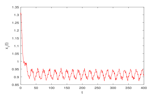
Figure 1: $\mathbb{T}=\mathbb{R}.$ Numerical solution $x_{1}(t)$ of system (4.1) for $(\varphi_{1}(t),\varphi_{2}(t),\varphi_{3}(t))=(1.3,1.3,1.5).$

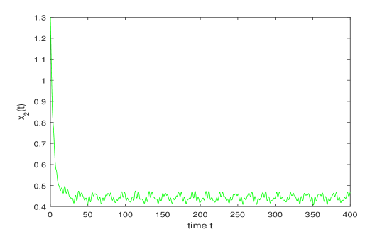
Figure 2: $\mathbb{T}=\mathbb{R}.$ Numerical solution $x_{2}(t)$ of system (4.1) for $(\varphi_{1}(t),\varphi_{2}(t),\varphi_{3}(t))=(1.3,1.3,1.5).$

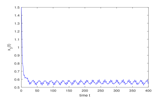
Figure 3: $\mathbb{T}=\mathbb{R}.$ Numerical solution $x_{3}(t)$ of system (4.1) for $(\varphi_{1}(t),\varphi_{2}(t),\varphi_{3}(t))=(1.3,1.3,1.5).$

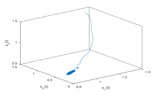
Figure 4: Continuous situation $(\mathbb{T}=\mathbb{R}):x_{1}(t),x_{2}(t),x_{3}(t)$.

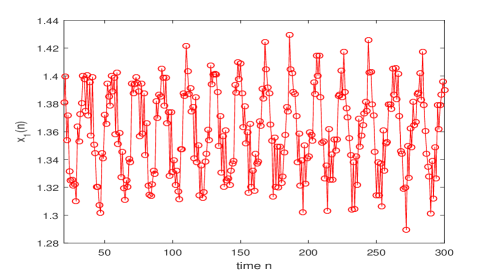
Figure 5: $\mathbb{T}=\mathbb{Z}.$ Numerical solution $x_{1}(n)$ of system (4.1) for $(\varphi_{1}(n),\varphi_{2}(n),\varphi_{3}(n))=(1.2,1.2,2.3).$

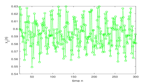
Figure 6: $\mathbb{T}=\mathbb{Z}.$ Numerical solution $x_{2}(n)$ of system (4.1) for $(\varphi_{1}(n),\varphi_{2}(n),\varphi_{3}(n))=(1.2,1.2,2.3).$

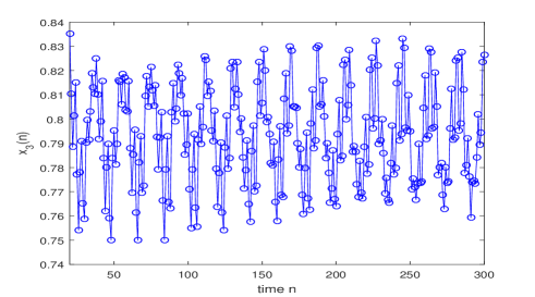
Figure 7: $\mathbb{T}=\mathbb{Z}.$ Numerical solution $x_{3}(n)$ of system (4.1) for $(\varphi_{1}(t),\varphi_{2}(t),\varphi_{3}(n))=(1.2,1.2,2.3).$

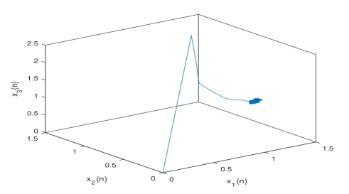
Figure 8: Discrete situation $(\mathbb{T}=\mathbb{R}):x_{1}(n),x_{2}(n),x_{3}(n)$.

6 Conclusion

In this paper, we proposed a new concept of almost periodic time scales, two new definitions of almost periodic functions on time scales and investigated some basic properties of them, which can unify the continuous and the discrete cases effectively. As an application, we obtain some sufficient conditions for the existence and exponential stability of positive almost periodic solutions for a class of Nicholson’s blowflies models on time scales. Our methods and results of this paper may be used to study almost periodicity of general dynamic equations on time scales. Besides, based on our this new concept of almost periodic time scales, one can further study the problems of pseudo almost periodic functions, pseudo almost automorphic functions and pseudo almost periodic set-valued functions on times as well as the problems of pseudo almost periodic, pseudo almost automorphic and pseudo almost periodic set-valued dynamic systems on times and so on.

References

- [1] A.J. Nicholson, An outline of the dynamics of animal populations, Aust. J. Zool. 2 (1954) 9-65.
- [2] W.S.C. Gurney, S.P. Blythe, R.M. Nisbet, Nicholson’s blowflies revisited, Nature 287 (1980) 17-21.
- [3] Y. Chen, Periodic solutions of delayed periodic Nicholson s blowflies models, Can. Appl. Math. Q. 11 (2003) 23-28.
- [4] J. Li, C. Du, Existence of positive periodic solutions for a generalized Nicholson s blowflies model, J. Comput. Appl. Math. 221 (2008) 226-233.
- [5] B.W. Liu, Global exponential stability of positive periodic solutions for a delayed Nicholson s blowflies model, J. Math. Anal. Appl. 412 (2014) 212-221.
- [6] S. Saker, S. Agarwal, Oscillation and global attractivity in a periodic Nicholson s blowflies model, Math. Comput. Modelling 35 (2002) 719-731.
- [7] Q. Zhou, The positive periodic solution for Nicholson-type delay system with linear harvesting terms, Appl. Math. Modelling 37 (2013) 5581-5590.
- [8] J.W. Li, C.X. Du, Existence of positive periodic solutions for a generalized Nicholson’s blowflies model, J. Comput. Appl. Math. 221 (2008) 226-233.
- [9] T.S. Yi, X. Zou, Global attractivity of the diffusive Nicholson blowflies equation with Neumann boundary condition: A non-monotone case, J. Differential Equations 245 (11) (2008) 3376-3388.
- [10] B. Liu, S. Gong, Permanence for Nicholson-type delay systems with nonlinear density-dependent mortality terms, Nonlinear Anal. Real World Appl. 12 (2011) 1931-1937.
- [11] B.W. Liu, Global stability of a class of Nicholson’s blowflies model with patch structure and multiple time-varying delays, Nonlinear Anal. Real World Appl. 11 (2010) 2557-2562.
- [12] J.Y. Shao, Global exponential stability of non-autonomous Nicholson-type delay systems, Nonlinear Anal. Real World Appl. 13 (2012) 790-793.
- [13] L. Berezansky, L. Idels, L. Troib, Global dynamics of Nicholson-type delay systems with applications, Nonlinear Anal. Real World Appl. 12 (1) (2011) 436-445.
- [14] W.T. Wang, L.J. Wang, W. Chen, Existence and exponential stability of positive almost periodic solution for Nicholson-type delay systems, Nonlinear Anal. Real World Appl. 12 (2011) 1938-1949.
- [15] T. Faria, Global asymptotic behaviour for a Nicholson model with patch structure and multiple delays, Nonlinear Anal. 74 (2011) 7033-7046.
- [16] J.O. Alzabut, Almost periodic solutions for an impulsive delay Nicholson’s blowflies model, J. Comput. Appl. Math. 234 (2010) 233-239.
- [17] W. Chen, B.W. Liu, Positive almost periodic solution for a class of Nicholson’s blowflies model with multiple time-varying delays, J. Comput. Appl. Math. 235 (2011) 2090-2097.
- [18] F. Long, Positive almost periodic solution for a class of Nicholson’s blowflies model with a linear harvesting term, Nonlinear Anal. Real World Appl. 13 (2012) 686-693.
- [19] L.J. Wang, Almost periodic solution for Nicholson’s blowflies model with patch structure and linear harvesting terms, Appl. Math. Modelling 37 (2013) 2153-2165.
- [20] X. Liu, J. Meng, The positive almost periodic solution for Nicholson-type delay systems with linear harvesting terms, Appl. Math. Modelling 36 (2012) 3289-3298.
- [21] Y.L. Xu, Existence and global exponential stability of positive almost periodic solutions for a delayed Nicholson’s blowflies model, J. Korean Math. Soc. 51 (2014) 473-493.
- [22] B.W. Liu, Positive periodic solutions for a nonlinear density-dependent mortality Nicholson s blowflies model, Kodai Math. J. 37 (2014) 157-173.
- [23] H.S. Ding, J. Alzabut, Existence of positive almost periodic solutions for a Nicholson’s blowflies model, Electron. J. Diff. Equ. 2015 (180) (2015) 1-6.
- [24] Z.J. Yao, Existence and exponential convergence of almost periodic positive solution for Nicholson’s blowflies discrete model with linear harvesting term, Math. Meth. Appl. Sci. 37 (2014) 2354-2362.
- [25] J.O. Alzabut, Existence and exponential convergence of almost periodic aolutions for a discrete Nicholson’s blowflies model with nonlinear harvesting term, Math. Sci. Lett. 2(3) (2013) 201-207.
- [26] S. Hilger, Analysis on measure chains–a unified approach to continuous and discrete calculus, Results Math. 18 (1990) 18-56.
- [27] Y.K. Li, L. Yang, Existence and stability of almost periodic solutions for Nicholson’s blowflies models with patch structure and linear harvesting terms on time scales, Asian-European J. Math. 5 (3) (2012) 1250038 (14 pages).
- [28] Y.K. Li, C. Wang, Uniformly almost periodic functions and almost periodic solutions to dynamic equations on time scales, Abstr. Appl. Anal. 2011 (2011), Article ID 341520, 22 pages.
- [29] Y. Li, C. Wang, Pseudo almost periodic functions and pseudo almost periodic solutions to dynamic equations on time scales, Adv. Difference Equ. 2012, 2012:77.
- [30] C. Lizama, J.G. Mesquita, Almost automorphic solutions of dynamic equations on time scales, J. Funct. Anal. 265 (2013) 2267-2311.
- [31] C. Wang, Y. Li, Weighted pseudo almost automorphic functions with applications to abstract dynamic equations on time scales, Ann. Polon. Math. 108 (2013) 225-240.
- [32] C. Wang, R.P. Agarwal, Weighted piecewise pseudo almost automorphic functions with applications to abstract impulsive dynamic equations on time scales, Adv. Difference Equ. 2014, 2014:153.
- [33] S.H. Hong, Y.Z. Peng, Almost periodicity of set-valued functions and set dynamic equations on time scales, Information Sciences 330 (2016) 157-174.
- [34] C. Lizama, J.G. Mesquita, Asymptotically almost automorphic solutions of dynamic equations on time scales, J. Math. Anal. Appl. 407 (2013) 339-349.
- [35] C. Lizama, J.G. Mesquita, R. Ponce, A connection between almost periodic functions defined on timescales and , Applic. Anal. 93 (2014) 2547-2558.
- [36] Y. Li, L. Yang, Almost automorphic solution for neutral type high-order Hopfield neural networks with delays in leakage terms on time scales, Appl. Math. Comput. 242 (2014) 679-693.
- [37] T. Liang, Y. Yang, Y. Liu, L. Li, Existence and global exponential stability of almost periodic solutions to Cohen-Grossberg neural networks with distributed delays on time scales, Neurocomputing 123 (2014) 207-215.
- [38] J. Gao, Q.R. Wang, L.W. Zhang, Existence and stability of almost-periodic solutions for cellular neural networks with time-varying delays in leakage terms on time scales, Appl. Math. Compu. 237 (2014) 639-649.
- [39] Z. Yao, Existence and global exponential stability of an almost periodic solution for a host-macroparasite equation on time scales, Adv. Difference Equ. 2015, 2015:41.
- [40] G. Mophou, G.M. N’Guérékata, A. Milce, Almost automorphic functions of order and applications to dynamic equations on time scales, Discrete Dyn. Nat. Soc. 2014 (2014), Article ID 410210, 13 pages.
- [41] H. Zhou, Z. Zhou, W. Jiang, Almost periodic solutions for neutral type BAM neural networks with distributed leakage delays on time scales, Neurocomputing 157 (2015) 223-230.
- [42] Y.K. Li, C. Wang, Almost periodic functions on time scales and applications, Discrete Dyn. Nat. Soc. 2011 (2011), Article ID 727068, 20 pages.
- [43] C. Wang, R.P. Agarwal, A further study of almost periodic time scales with some notes and applications, Abstr. Appl. Anal. 2014 (2014), Article ID 267384, 11 pages.
- [44] Y.K. Li, B. Li, Almost periodic time scales and almost periodic functions on time scales, J. Appl. Math. 2015 (2015), Article ID 730672, 8 pages.
- [45] Y.K. Li, L.L. Zhao, L. Yang, -Almost periodic solutions of BAM neural networks with time-varying delays on time scales, The Scientific World J. 2015 (2015), Article ID 727329, 15 pages.
- [46] Y.K. Li, B. Li, X.F. Meng, Almost automorphic funtions on time scales and almost automorphic solutions to shunting inhibitory cellular neural networks on time scales, J. Nonlinear Sci. Appl. 8 (2015) 1190-1211.
- [47] M. Bohner, A. Peterson, Dynamic Equations on Time Scales, An Introduction with Applications, Boston: Birkhäuser; 2001.
- [48] A.M. Fink, Almost Periodic Differential Equations, Springer-Verlag, Berlin, 1974.
- [49] A.M. Fink, G. Seifert, Liapunov functions and almost periodic solutions for almost periodic systems, J. Differential Equations 5 (1969) 307-313.
- [50] C. David, M. Cristina, Invariant manifolds, global attractors and almost periodic solutions of nonautonomous defference equations, Nonlinear Anal. 56(4) (2004) 465-484.
- [51] J.K. Hale, S.M. Verduyn Lunel, Introduction to Functional Differential Equations, Springer-Verlag, New York, 1993.