Progressive EM for Latent Tree Models and Hierarchical Topic Detection
Abstract
Hierarchical latent tree analysis (HLTA) is recently proposed as a new method for topic detection. It differs fundamentally from the LDA-based methods in terms of topic definition, topic-document relationship, and learning method. It has been shown to discover significantly more coherent topics and better topic hierarchies. However, HLTA relies on the Expectation-Maximization (EM) algorithm for parameter estimation and hence is not efficient enough to deal with large datasets. In this paper, we propose a method to drastically speed up HLTA using a technique inspired by recent advances in the moments method. Empirical experiments show that our method greatly improves the efficiency of HLTA. It is as efficient as the state-of-the-art LDA-based method for hierarchical topic detection and finds substantially better topics and topic hierarchies.
1 INTRODUCTION
Detecting topics and topic hierarchies from document collections, along with its many potential applications, is a major research area in Machine Learning. Currently the predominant approach to topic detection is latent Dirichlet allocation (LDA) (Blei et al., 2003). LDA has been developed to detect topics and to model relationships among them, including topic correlations (Blei and Lafferty, 2007), topic hierarchies (Blei et al., 2010; Paisley et al., 2012), and topic evolution (Blei and Lafferty, 2006). We collectively name these methods LDA-based methods. In those methods, a topic is a probability distribution over a vocabulary and a document is a mixture of topics. Therefore LDA is a type of mixture membership model.
A totally different approach to hierarchical topic detection is recently proposed by Liu et al. (2014). It is called hierarchical latent tree analysis (HLTA), where topics are organized hierarchically as a latent tree model (LTM) (Zhang, 2004; Zhang et al., 2008b) such as the one in Fig 1. In HLTA, a topic is a state of a latent variable and it corresponds to a collection of documents, and a document can belong to multiple topics. HLTA is therefore a type of multiple membership model.
Empirical results from Liu et al. (2014) indicate that HLTA finds significantly better topics and topic hierarchies than hierarchical latent Dirichlet allocation (hLDA), the first LDA-based method for hierarchical topic detection. However, HLTA does not scale up well. It took, for instance, 17 hours to process a NIPS dataset that consists of fewer than 2,000 documents over 1,000 distinct words (Liu et al., 2014).(Note that hLDA took even longer time.)
The computational bottleneck of HLTA lies in the use of the EM algorithm (Dempster et al., 1977) for parameter estimation. In this paper, we propose progressive EM (PEM) as a replacement of EM so as to scale up HLTA. PEM is motivated by the moments method, where parameters are determined by solving equations, each of which involves a small number of model parameters related to two or three observed variables (Chang, 1996; Anandkumar et al., 2012). Similarly, PEM works in steps and, at each step, it focuses on a small part of the model parameters and involves only three or four observed variables.
Our new algorithm is hence named PEM-HLTA. It is drastically faster than HLTA. PEM-HLTA finished processing the aforementioned NIPS dataset within 4 minutes. It only took around 11 hours, on a single desktop computer, to analyze a version of New York Times dataset that consists of 300,000 articles with 10,000 distinct words. PEM-HLTA is also as efficient as nHDP (Paisley et al., 2012), a state-of-the-art LDA-based method for hierarchical topic detection, and it significantly outperforms nHDP, as well as hLDA, in terms of the quality of topics and topic hierarchies.
2 PRELIMINARIES
A latent tree model (LTM) is a Markov random field over an undirected tree, where the leaf nodes represent observed variables and the internal nodes represent latent variables (Zhang et al., 2008a). In this paper we assume all variables have finite cardinality, i.e., finite number of possible states.
Parameters of an LTM consist of potentials associated with edges and nodes such that the product of all potentials is a joint distribution over all variables. We pick the potentials as follows: Root the model at an arbitrary latent node, direct the edges away from the root, and specify a marginal distribution for the root and a conditional distribution for each of the other nodes given its parent. Then in Fig 2(b), if is the root, the parameters are the distributions , and so forth. Because of the way the potentials are picked, LTMs are technically tree-structured Bayesian networks (Pearl, 1988).
LTMs with a single latent variables are known as latent class models (LCMs)(Bartholomew and Knott, 1999). They are a type of finite mixture models for discrete data. For example, the model in Fig 2(a) defines the following mixture distribution over the observed variables:
| (1) |
where is the cardinality of . If the model is learned from a dataset, then the data are partitioned into soft clusters, each represented by a state of . The model in Fig 2(b) has two latent variables. Its joint distribution can be reduced to two different but related mixture distributions:
The model gives two different ways of partitioning the data, one represented by and the other by . Hence LTMs are a tool for multidimensional clustering (Chen et al., 2012).
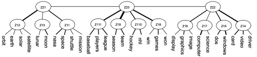 Figure 1: Latent tree model obtained from a toy text dataset.
![]() (a)
(a)
![]() (b)
(b)
3 THE ALGORITHM
The input to our PEM-HLTA algorithm is a collection of documents, each represented as a binary vector over a vocabulary . The values in the vector indicate the presence or absence of words in the document. The output is an LTM, such as the one shown in Fig 1, where the word variables are at the bottom and the latent variables, all assumed binary, form several levels of hierarchy on top. Each state of a latent variable corresponds to a cluster of documents and is interpreted as a topic. The top level control of PEM-HLTA is given in Algorithm 1, and subroutines in Algorithms 2–3.
3.1 TOP LEVEL CONTROL
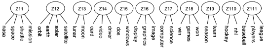
We illustrate the top level control using the example model in Fig 1, which is learned from a dataset with 30 word variables. In the first pass through the loop, the subroutine BuildIslands is called (line 3). It partitions all variables into 11 clusters (Fig 3 bottom), which are uni-dimensional in the sense that the co-occurrences of words in each cluster can be properly modeled using a single latent variable. A latent variable is introduced for each cluster to form an LCM. We metaphorically refer to the LCMs as islands and the latent variables in them as level-1 latent variables.
The next step is to link up the 11 islands (line 4). This is done by estimating the mutual information (MI) (Cover and Thomas, 2012) between every pair of latent variables and building a Chow-Liu tree (Chow and Liu, 1968) over them, so as to form an overall model (Liu et al., 2013). The result is the model at the middle of Fig 3.
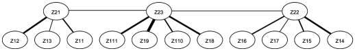
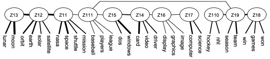
In the subroutine HardAssignment, inference is carried out to compute the posterior distribution of each latent variable for each document. The document is assigned to the state with the maximum posterior probability. This results in a dataset over the level-1 latent variables (line 10). In the second pass through the loop, the level-1 latent variables are partitioned into 3 groups and 3 islands are created. The islands are linked up to form the model shown at the top of Fig 3. At line 8, the model at the top of Fig 3 () is stacked on the model in the middle () to give rise to the final model in Fig 1. While doing so, the subroutine StackModels cuts off the links among the level-1 latent variables. The number of nodes at the top level is below the threshold , if we set , and hence the loop is exited. EM is run on the final model for steps to improve its parameters (line 12). In our experiments, we set . In Section 5.1 we will discuss how to extract a topic hierarchy from the final model.
- Inputs:
-
—Collection of documents, —Upper bound on the number of top-level topics, —Threshold used in UD-test, —Number of EM steps on final model.
- Outputs:
-
An HLTM and a topic hierarchy.
3.2 BUILDING ISLANDS
The pseudo code for the subroutine BuildIslands is given in Algorithm 2. It calls another subroutine OneIsland to identify a uni-dimensional subset of observed variables and builds an LCM with them. Then it repeats the process on those observed variables left to create more islands, until all variables are included in these islands. Finally, it returns the set of all the islands.
3.2.1 UNI-DIMENSIONALITY TEST
We rely on the uni-dimensionality test (UD-test) (Liu et al., 2013) to determine whether a set of variables is uni-dimensional. The idea is to compare two LTMs and , where is the best model among all LCMs for while is the best model among all LTMs that contain two latent variables. The model selection criterion used is the BIC score (Schwarz, 1978). The set is uni-dimensional if the following inequality holds:
| (2) |
where is a threshold. In other words, is considered uni-dimensional if the best two-latent variable model is not significantly better than the best one-latent variable model. The quantity on the left hand side of Equation (2) is a large sample approximation of the natural logarithm of Bayes factor (Raftery, 1995) for comparing and . According to the cut-off values for the Bayes factor, we set in our experiments.
3.2.2 BUILDING AN ISLAND
Given dataset with variables , the subroutine OneIsland identifies a uni-dimensional subset of variables and builds an LCM for them. Define the mutual information between a variable and a set as . OneIsland maintains a working set of observed variables. Initially, contains the pair of variables with the highest MI among all pairs, and a third variable that has the highest MI with the pair (line 2). At line 5, an LCM is learned for those three variables using the subroutine LearnLCM, which is given in the Appendix along with some other subroutines. Then other variables are added to one by one until the UD-test fails.
We illustrate this process using Fig 2. Suppose initially consists of three variables , , . Let be the variable that has the maximum MI with among all other variables. Suppose the UD-test passes on , then is added to . Next let be the variable with the maximum MI with S (line 7) and the UD-test is performed on (lines 8-14). The two models and used in the test is shown in Fig 2. For computational efficiency, we do not search for the best structure for . Instead, the structure is determined as follows: Pick the variable in that has the maximum MI with (line 8) (let it be ), and group it with in the model (line 12). The model parameters are estimated using the subroutines PEM-LCM and PEM-LTM-2L, which will be explained in the next section. If the test fails, then , and are removed from , and what remains in the model, an LCM, is returned. If the test passes, is added to (line 16) and the process continues.
4 PROGRESSIVE EM FOR MODEL CONSTRUCTION
PEM-HLTA conceptually consists of a model construction phase (lines 2-11) and a parameter estimation phase (line 12). During the first phase, many intermediate models are constructed. In this section, we present a fast method for estimating the parameters of those intermediate models.
4.1 MOMENTS METHOD FOR PARAMETER ESTIMATION
We begin by presenting a property of LTMs that motivates our new method. A similar property of HMMs was first discovered by Chang (1996). We introduce some notations using of Fig 2. Since all variables have the same cardinality, the conditional distribution can be regarded as a square matrix, which we denote as . Similarly, is the matrix representation of the joint distribution . For a value of , is the vector presentation of and the matrix representation of .
Theorem 1
[ Zhang et al. (2014)] Let be the latent variable in an LCM and be three of the observed variables. Assume all variables have the same cardinality and the matrices and are invertible. Then we have
| (3) |
where is a diagonal matrix with components of as the diagonal elements.
The equation implies that the model parameters are the eigenvalues of the matrix on the right, and hence can be obtained from the marginal distributions .
Theorem 1 can be used to estimate under two conditions: (1) There is a good fit between the data and model as if the data were generated from the model, and (2) the sample size is sufficiently large. In this case, the empirical marginal distributions and computed from data are accurate estimates of the distributions and of the model. We can use them to form the matrix , and determine as the eigenvalues of the matrix. This is called the moments method. Note that Theorem 1 still applies when replacing edges like with paths. For example in Fig 2(b), if and are to be estimated, a third observed variable can be chosen from as long as there is path from to this observed variable.
Theorem 1 can be also used to estimate all the parameters of the model in Fig 2. First, we can estimate using Equation 3 in the sub-model -. By swapping the roles of variables, we can also estimate and in the sub-model. Next we can consider the sub-model - and estimate with and fixed. Finally, we can consider the sub-model - and estimate there with and fixed. Note that the parameters are estimated in steps instead of all at once. Hence we call this scheme progressive parameter estimation.
4.2 PROGRESSIVE EM
The moments method is not iterative and hence can be drastically faster than EM. Unfortunately, it does not produce high quality estimates when the model does not fit data well and/or the sample size is not sufficiently large. In such cases, the empirical marginal distributions and are poor estimates of the distributions and of the model. In our experiences, the method frequently gives negative estimates for probability values in the context of latent tree models.
In this paper, we do not estimate parameters by solving the equation in Theorem 1. However, we adopt the progressive estimation scheme and combine it with EM. This gives rise to progress EM (PEM). To estimate the parameters of , PEM first estimates , , , and by running EM on the sub-model -; then it estimates by running EM on the sub-model - with , and fixed; and finally it estimates on sub-model - similarly. All the sub-models involve 3 observed variables.
For , PEM first estimates , , and by running EM on sub-model -; then it estimates , and by running EM on the two latent variable sub-model ---, with , and fixed. Note that only two of the children of are used here, and the model involves only 4 observed variables.
Intuitively, the moments method tries to fit data in a rigid way, while PEM tries to fit data in an elastic manner. It never gives negative probability values. Moreover, it is still efficient because EM is run only on sub-models with three or four observed binary variables, and local maxima is seldom an issue using multiple starting points.
4.3 PEM FOR ISLAND BUILDING
PEM can be aligned with the subroutine OneIsland nicely because the subroutine adds variables to the working set one at a time. Consider a pass through the loop. At the beginning, we have an LCM for the variables in , whose parameters have been estimated earlier. Then OneIsland finds the variable outside that has the maximum MI with , and the variable inside that has the maximum MI with (line 7, 8).
At line 11, OneIsland adds to the to create a new LCM , and estimates the parameters for the new variable using the subroutine PEM-LCM. We illustrate how this is done using Fig 2. Suppose the LCM is the model - and the variable is . PEM-LCM adds the variable to and thereby creates a new LCM , which is - (Fig 2 left). To estimate the distribution , PEM-LCM creates a temporary model from by only keeping three observed variables: and two other variables with maximum MI with . Suppose is -. PEM-LCM estimates the distribution by running EM on with all other parameters fixed. Finally, it copies from to , and returns .
At line 12, OneIsland adds to and learns a two-latent variable model using the subroutine PEM-LTM-2L. We illustrate PEM-LTM-2L using the foregoing example. Let be and be . PEM-LTM-2L creates the new model , which is --- (Fig 2 right). To estimate the parameters , and , PEM-LTM-2L creates a temporary model which is ---. Only the two of the children of that have maximum MI with remain( and in this example). PEM-LTM-2L estimates the three distributions by running EM on with all other parameters fixed. Finally, it copies the distributions from to and returns . 111Details of PEM-LCM and PEM-LTM-2L can be found in the Appendix submitted as a supplement. Similarly in the subroutine BridgedIslands we use this method to estimate parameters for edges between latent variables, but only estimating and keeping all other parameters fixed.
5 EMPIRICAL RESULTS
We aim at scaling up HLTA, hence we need to empirically determine how efficient PEM-HLTA is compared with HLTA. We also compare PEM-HLTA with nHDP, the state-of-the-art LDA-based method for hierarchical topic detection, in terms of computational efficiency and quality of results. Also included in the comparisons are hLDA and a method named CorEx (Ver Steeg and Galstyan, 2014) that builds hierarchical latent trees by optimizing an information-theoretic objective function.
Two of the datasets used are NIPS data222http://www.cs.nyu.edu/ roweis/data.html and Newsgroup333http://qwone.com/˜jason/20Newsgroups/. Three versions of the NIPS data with vocabulary sizes 1,000, 5,000 and 10,000 were created by choosing words with highest average TF-IDF values, referred to as Nips-1k, Nips-5k and Nips-10k. Similarly, two versions (News-1k and News-5k) of the Newsgroup data were created. Note that News-10k is not included because it is beyond the capabilities of three of the methods. Comparisons of PEM-HLTA and nHDP on large-scale data will be given separately in Section 5.4. After preprocessing, NIPS and Newsgroup consist of 1,955 and 19,940 documents respectively. For PEM-HLTA, HLTA and CorEx, the data are represented as binary vectors, whereas for nHDP and hLDA, they are represented as bags-of-words.
PEM-HLTA determines the height of hierarchy and the number of nodes at each level automatically. On the NIPS and Newsgroup datasets, it produced hierarchies with between 4 to 6 levels. For nHDP and hLDA, the height of hierarchy needs to be manually set and is usually set at 3. We set the number of nodes at each level in such way that nHDP and hLDA would yield roughly the same total number of topics as PEM-HLTA. CorEx were configured similarly. PEM-HLTA is implemented in Java. The parameter settings are described in Section 3. Implementations of other algorithms were provided by their authors and ran at their default parameter settings. All experiments are conducted on the same desktop computer.
5.1 TOPIC HIERARCHIES FOR NIPS-10K
Table 1 shows parts of the topic hierarchies obtained by nHDP and PEM-HLTA. The left half displays 3 top-level topics by nHDP and their children. Each nHDP topic is represented using the top 5 words occurring with highest probabilities in the topic. The right half show 3 top-level topics yielded by PEM-HLTA and their children. The topics are extracted from the model learned by PEM-HLTA as follows: For a latent binary variable in the model, we enumerate the word variables in the sub-tree rooted at Z in descending order of their MI values with Z. The leading words are those whose probabilities differ the most between the two states of and are hence used to characterize the states. The state of under which the words occur less often overall is regarded as the background topic and is not reported, while the other state is reported as a genuine topic. Values in [] show the percentage of the documents belonging to the genuine topic.
Let us examine some of the topics. We refer to topics on the left using the letter ‘L’ followed by topic numbers and those on the right using ‘R’. For PEM-HLTA, R1 consists of probability terms: R1.1 is about EM algorithm; R1.2 about Gaussian mixtures and R1.3 about generative distributions. R1.4 is a combination of variance and noise, which are separated at the next lower level. For nHDP, the topic L1 and its children L1.1, L1.2 and L1.5 are also about probability. However, L1.3 and L1.4 do not fit in the group well. The topic R2 is about image analysis, while its first four subtopics are about different aspects of image analysis: sources of images, pixels, objects. R2.5 and R2.6 are also meaningful and related, but do not fit in well. They are placed in another subgroup by PEM-HLTA. In nHDP, the subtopics of L2 do not give a clear spectrum of aspects of image analysis. The topic R3 is about speech recognition. Its subtopics are about different aspects of speech recognition. Only R3.4 does not fit in the group well. In contrast, L3 and its subtopics do not present a clear semantic hierarchy. Some of them are not meaningful. Another topic related to speech recognition L1.5 is placed elsewhere. Overall, the topics and topic hierarchy obtained by PEM-HLTA are more meaningful than those by nHDP.
|
|
5.2 TOPIC COHERENCE AND MODEL QUALITY
To quantitatively measure the quality of the topics, we use the topic coherence score proposed by Mimno et al. (2011). The metric depends on the number of words used to characterize a topic. We set . In addition, we use held-out likelihood to assess the quality of the models produced by the five algorithms. Each dataset was randomly partitioned into a training set with 80% of the data, and a test set with 20% of the data.
Table 2 shows the average topic coherence scores of the topics produced by the five algorithms. The sign “-” indicates running time exceeded 72 hours. The quality of topics produced by PEM-HLTA is similar to those by HLTA on Nips-1k and News-1k, and better on Nips-5k. In all cases, PEM-HLTA produced significantly better topics than nHDP and the other two algorithms. The held-out per-document loglikelihood statistics are shown in Table 3. The likelihood values of PEM-HLTA are similar to those of HLTA, showing that the use of PEM to replace EM does not influence model quality much. They are significantly higher than those of CorEx. Note that the likelihood values in Table 3 for the LDA-based methods are calculated from bag-of-words data. They are still lower than the other methods even calculated from the same binary data as for the other three methods.
It should be noted that, in general, better model fit does not necessarily imply better topic quality (Chang et al., 2009). In context of hierarchical topic detection, however, PEM-HLTA not only leads to better model fit, but also gives better topics and better topic hierarchies. Table 2: Average topic coherence scores. Nips-1k Nips-5k Nips-10k News-1k News-5k PEM-HLTA -6.25 -8.04 -8.87 -12.30 -13.07 HLTA -6.23 -9.23 — -12.08 — hLDA -6.99 -8.94 — — — nHDP -8.08 -9.55 -9.86 -14.26 -14.51 CorEx -7.23 -9.85 -10.64 -13.47 -14.51 Table 3: Per-document loglikelihood Nips-1k Nips-5k Nips-10k News-1k News-5k PEM-HLTA -390 -1,117 -1,424 -116 -262 HLTA -391 -1,161 — -120 — hLDA -1,520 -2,854 — — — nHDP -3,196 -6,993 -8,262 -265 -599 CorEx -442 -1,226 -1,549 -140 -322
5.3 RUNNING TIMES
Table 4 shows the running time statistics. PEM-HLTA drastically outperforms HLTA, and the difference increases with vocabulary size. On Nips-10k and News-5k, HLTA did not terminate in 3 days, while PEM-HLTA finished the computation in about 6 hours. PEM-HLTA is also faster than nHDP, although the difference decreases with vocabulary size as nHDP works in a stochastic way (Paisley et al., 2012). Moreover, PEM-HLTA is more efficient than hLDA and CorEx.
| Time(min) | Nips-1k | Nips-5k | Nips-10k | News-1k | News-5k |
|---|---|---|---|---|---|
| PEM-HLTA | 4 | 140 | 340 | 47 | 365 |
| HLTA | 42 | 2,020 | — | 279 | — |
| hLDA | 2,454 | 4,039 | — | — | — |
| nHDP | 359 | 382 | 435 | 403 | 477 |
| CorEx | 43 | 366 | 704 | 722 | 4,025 |
| Time (min) | Average topic coherence | |
|---|---|---|
| PEM-HLTA | 670 | -12.86 |
| hHDP | 637 | -13.35 |
5.4 STOCHASTIC EM
Conceptually, PEM-HLTA has two phases: hierarchical model construction and parameter estimation. In the second phase, EM is run a predefined number of steps from the initial parameter values from the first phase. It is time-consuming if the sample size is large. Paisley et al. (2012) faced a similar problem with nHDP. They solve the problem using stochastic inference. The idea is to divide the data set into subsets and process the subsets one by one. Model parameters are updated after processing each data subset and overall one goes through the entire data set only once.We adopt the same idea for the second phase of PEM-HLTA and call it stochastic EM. We tested the idea on the New York Times dataset111http://archive.ics.uci.edu/ml/datasets/Bag+of+Words, which consists of 300,000 articles. To analyze the data, we picked 10,000 words using TF-IDF and then randomly divided the dataset into 50 equal-sized subsets. We used only the fist subset for the first phase of PEM-HLTA. For the second phase, we ran EM on current model once using each subset in turn until all the subsets are utilized .
On New York Times data, we only compare PEM-HLTA with nHDP since other methods are not amenable to processing large datasets as we can observe from Table 4. We still trained nHDP model using documents in bag-of-words form and PEM-HLTA using documents as binary vectors of words. Table 5 reports the running times and topic coherence. PEM-HLTA took around 11 hours which is a little bit slower than nHDP (10.5 hours). However, PEM-HLTA produced more coherent topics, which is not only testified by the coherence score, but also the resulting topic hierarchies. The reader could get a clear picture of the superiority of PEM-HLTA over nHDP by taking a quick look at the model structure and topic hierarchies submitted as supplements.
6 CONCLUSIONS
We have proposed and investigated a method to scale up HLTA — a newly emerged method for hierarchical topic detection. The key idea is to replace EM using progressive EM. The resulting algorithm PEM-HLTA reduces the computation time of HLTA drastically and can handle much larger datasets. More importantly, it outperforms nHDP, the state-of-the-art LDA-based method for hierarchical topic detection, in terms of both quality of topics and topic hierarchy, with comparable speed on large-scale data. Although we only show how PEM works in HLTA, PEM can possibly be used in other more general models. PEM-HLTA can also be further scaled up through parallelization and used for text classification. We plan to investigate these directions in the future.
References
- Anandkumar et al. (2012) Animashree Anandkumar, Kamalika Chaudhuri, Daniel Hsu, Sham M. Kakade, Le Song, and Tong Zhang. Spectral methods for learning multivariate latent tree structure. In Advances in Neural Information Processing Systems, pages 2025–2033, 2012.
- Bartholomew and Knott (1999) David J. Bartholomew and Martin Knott. Latent Variable Models and Factor Analysis. Arnold, 2nd edition, 1999.
- Blei and Lafferty (2006) David M Blei and John D Lafferty. Dynamic topic models. In Proceedings of the 23rd international conference on Machine learning, pages 113–120. ACM, 2006.
- Blei and Lafferty (2007) David M Blei and John D Lafferty. A correlated topic model of science. The Annals of Applied Statistics, pages 17–35, 2007.
- Blei et al. (2003) David M. Blei, Andrew Y. Ng, and Michael I. Jordan. Latent Dirichlet allocation. Journal of Machine Learning Research, 3:993–1022, 2003.
- Blei et al. (2010) David M. Blei, Thomas L. Griffiths, and Michael I. Jordan. The nested Chinese restaurant process and Bayesian nonparametric inference of topic hierarchies. Journal of the ACM, 57(2):7:1–7:30, 2010.
- Chang et al. (2009) Jonathan Chang, Jordan L Boyd-Graber, Sean Gerrish, Chong Wang, and David M Blei. Reading tea leaves: How humans interpret topic models. In Advances in Neural Information Processing Systems, volume 22, pages 288–296, 2009.
- Chang (1996) Joseph T. Chang. Full reconstruction of Markov models on evolutionary trees: Identifiability and consistency. Mathematical Biosciences, 137(1):51–73, 1996.
- Chen et al. (2012) Tao Chen, Nevin L. Zhang, Tengfei Liu, Kin Man Poon, and Yi Wang. Model-based multidimensional clustering of categorical data. Artificial Intelligence, 176:2246–2269, 2012.
- Chow and Liu (1968) C. K. Chow and C. N. Liu. Approximating discrete probability distributions with dependence trees. IEEE Transactions on Information Theory, 14(3):462–467, 1968.
- Cover and Thomas (2012) Thomas M Cover and Joy A Thomas. Elements of information theory. John Wiley & Sons, 2012.
- Dempster et al. (1977) Arthur P. Dempster, Nan M. Laird, and Donald B. Rubin. Maximum likelihood from incomplete data via the EM algorithm. Journal of the Royal Statistical Society. Series B (Methodological), 39(1):1–38, 1977.
- Liu et al. (2013) Teng-Fei Liu, Nevin L. Zhang, Peixian Chen, April Hua Liu, Leonard K.M. Poon, and Yi Wang. Greedy learning of latent tree models for multidimensional clustering. Machine Learning, 98(1–2):301–330, 2013.
- Liu et al. (2014) Tengfei Liu, Nevin L. Zhang, and Peixian Chen. Hierarchical latent tree analysis for topic detection. In Machine Learning and Knowledge Discovery in Databases, pages 256–272, 2014.
- Mimno et al. (2011) David Mimno, Hanna M Wallach, Edmund Talley, Miriam Leenders, and Andrew McCallum. Optimizing semantic coherence in topic models. In Proceedings of the Conference on Empirical Methods in Natural Language Processing, pages 262–272. Association for Computational Linguistics, 2011.
- Paisley et al. (2012) John Paisley, Chong Wang, David M Blei, and Michael I Jordan. Nested hierarchical dirichlet processes. IEEE Transactions on Pattern Analysis and Machine Intelligence, 37, 2012.
- Pearl (1988) Judea Pearl. Probabilistic Reasoning in Intelligent Systems: Networks of Plausible Inference. Morgan Kaufmann Publishers, San Mateo, California, 1988.
- Raftery (1995) Adrian E. Raftery. Bayesian model selection in social research. Sociological Methodology, 25:111–163, 1995.
- Schwarz (1978) Gideon Schwarz. Estimating the dimension of a model. The Annals of Statistics, 6(2):461–464, 1978.
- Ver Steeg and Galstyan (2014) Greg Ver Steeg and Aram Galstyan. Discovering structure in high-dimensional data through correlation explanation. In Advances in Neural Information Processing Systems 27, pages 577–585, 2014.
- Zhang (2004) Nevin L. Zhang. Hierarchical latent class models for cluster analysis. Journal of Machine Learning Research, 5:697–723, 2004.
- Zhang et al. (2008a) Nevin L. Zhang, Yi Wang, and Tao Chen. Latent tree models and multidimensional clustering of categorical data. Technical Report HKUST-CS08-02, The Hong Kong Univeristy of Science and Technology, 2008a.
- Zhang et al. (2008b) Nevin L. Zhang, Yi Wang, and Tao Chen. Discovery of latent structures: Experience with the CoIL challenge 2000 data set. Journal of Systems Science and Complexity, 21:172–183, 2008b.
- Zhang et al. (2014) Nevin L. Zhang, Xiaofei Wang, and Peixian Chen. A study of recently discovered equalities about latent tree models using inverse edges. In Probabilistic Graphical Models, pages 567–580, 2014.