ASTEROSEISMIC ANALYSIS OF KEPLER TARGET KIC 2837475

Abstract

The ratios $r_{01}$ and $r_{10}$ of small to large separations of KIC 2837475 primarily exhibit an increase behavior in the observed frequency range. The calculations indicate that only the models with overshooting parameter $\delta_{\rm ov}$ between approximately 1.2 and 1.6 can reproduce the observed ratios $r_{01}$ and $r_{10}$ of KIC 2837475. The ratios $r_{01}$ and $r_{10}$ of the frequency separations of p-modes with inner turning points that are located in the overshooting region of convective core can exhibit an increase behavior. The frequencies of the modes that can reach the overshooting region decrease with the increase in $\delta_{\rm ov}$. Thus the ratio distributions are more sensitive to $\delta_{\rm ov}$ than to other parameters. The increase behavior of the KIC 2837475 ratios results from a direct effect of the overshooting of convective core. The characteristic of the ratios provides a strict constraint on stellar models. Observational constraints point to a star with $M=1.490\pm 0.018$ $M_{\odot}$, $R=1.67\pm 0.01$ $R_{\odot}$, age $=2.8\pm 0.4$ Gyr, and $1.2\lesssim\delta_{\rm ov}\lesssim 1.6$ for KIC 2837475.

1 Introduction

By comparing observed oscillation frequencies and the ratios of small to large separations with those calculated from theoretical models, asteroseismology imposes strict constraints on stellar models. The small separations are defined as (Roxburgh & Vorontsov, 2003)

$$d_{10}(n)\equiv-\frac{1}{2}(-\nu_{n,0}+2\nu_{n,1}-\nu_{n+1,0})$$ (1)

and

$$d_{01}(n)\equiv\frac{1}{2}(-\nu_{n,1}+2\nu_{n,0}-\nu_{n-1,1}).$$ (2)

In calculation, equations (1) and (2) are generally rewritten as the smoother five-point separations.

Asteroseismology has proved to be a powerful tool for determining fundamental star parameters, diagnosing internal structures of stars, and probing physical processes in stellar interiors (Eggenberger et al., 2005; Yang & Bi, 2007b; Stello et al., 2009; Christensen-Dalsgaard & Houdek, 2010; Yang et al., 2010, 2011a, 2012; Silva Aguirre et al., 2011, 2013; Liu et al., 2014; Chaplin et al., 2014; Metcalfe et al., 2014; Guenther et al., 2014).

F-type main-sequence (MS) stars usually have a convective core and a convective envelope. Consequently, they have various characteristics that are similar to that of the Sun, such as oscillations. On the other hand, they have peculiar properties due to the convective core that leads to a large gradient of chemical compositions at the bottom of the radiative region and an overshooting of the core in their interior. The overshooting of convective core extends the region of chemical mixing by a distance $\delta_{\rm ov}$$Hp$ above the top of the convective core that is determined by Schwarzchild criterion, where $Hp$ is the local pressure scale height and $\delta_{\rm ov}$ is a free parameter. Consequently, the overshooting of the core brings more H-rich material into the core, which prolongs the lifetime of the burning of core hydrogen, enhances the He-core mass left behind, and strongly changes the global characteristics of the following giant stages (Schr$\ddot{o}$der et al., 1997; Yang et al., 2012), such as the critical mass of He-flash and the global oscillation properties of red-clump stars (Yang et al., 2012).

The parameter $\delta_{\rm ov}$ has been observationally estimated in several ways. Prather & Demarque (1974) and Demarque et al. (1994) found that the value of $\delta_{\rm ov}$ is approximately 0.1-0.2 by comparing the theoretical and observational color-magnitude diagram of clusters. In addition, the value of $\delta_{\rm ov}$ estimated by matching the exact properties of certain $\zeta$ Aurigae eclipsing binaries is roughly 0.2-0.3 (Schr$\ddot{o}$der et al., 1997). The uncertainty of the mass and extension of the convective core due to overshooting directly affects the determination of the global parameters of stars by asteroseismology or other studies based on stellar evolution (Mazumdar et al., 2006). Thus determining the presence of the convective core and its extension is important for understanding the structure and evolution of stars.

The p-modes with $l=1$ penetrate more deeply into stellar interiors than the higher-$l$ modes. Thus, the ratios $r_{01}$ and $r_{10}$ are a potential tool for probing the existence and extension of a convective core of stars. Many authors (Mazumdar et al., 2006; Cunha & Metcalfe, 2007; Deheuvels et al., 2010; De Meulenaer et al., 2010; Silva Aguirre et al., 2011, 2013; Liu et al., 2014; Guenther et al., 2014; Tian et al., 2014) have studied the overshooting of convective cores by asteroseismology. Tian et al. (2014) gave that the value of $\delta_{\rm ov}$ is in the range of 0.0-0.2 for KIC 6225718. Liu et al. (2014) found that it is in the range of 0.4 and 0.8 for HD 49933; however, Guenther et al. (2014) obtained the $\delta_{\rm ov}$ for Procyon in the range of 0.9 and 1.5, which is much larger than the generally accepted value. This large $\delta_{\rm ov}$ may exist in other stars, and if this large $\delta_{\rm ov}$ is confirmed in more stars, the general understanding of the structure and evolution of stars will be improved to a certain degree.

Moreover, although the increase behaviors in the ratios of KIC 6106415 and KIC 12009504 arise from the low signal-to-noise ratio and the larger linewidth at the high-frequency end (Silva Aguirre et al., 2013), the increase in the ratios of HD 49933 at high frequencies may result from the effects of overshooting of convective core (Liu et al., 2014). Liu et al. (2014) argued that the gradient of the mean molecule weight in the radiative region hinders the propagation of p-modes, while the hindrance does not exist in the convective core. Therefore, the ratios $r_{01}$ and $r_{10}$ can exhibit an increase with frequencies when the inner turning points of the corresponding modes with $l=1$ are located in the overshooting region.

Individual frequencies of p-modes of dozens of MS stars have been extracted by Appourchaux et al. (2012), which provides an opportunity for studying the overshooting of the convective core and the behaviors of ratios $r_{01}$ and $r_{10}$. In these stars, the ratios $r_{01}$ and $r_{10}$ of KIC 2837475 increase linearly with a frequency in the range of approximately 1050 and 1600 $\mu$Hz, which may be related to the overshooting of convective core. The mass of KIC 2837475 estimated by Chaplin et al. (2014) is $1.41^{+0.06}_{-0.04}$ $M_{\odot}$ for the constraints of the spectroscopic $T_{\rm eff}$ and [Fe/H] of Bruntt et al. (2012) or $1.47^{+0.15}_{-0.13}$ $M_{\odot}$ for the constraints of the IRFM $T_{\rm eff}$ and field-average [Fe/H]. Moreover, Metcalfe et al. (2014) determined the value to be $1.39\pm 0.06$ $M_{\odot}$ for KIC 2837475.

In this work, we focus mainly on whether the observed characteristics of KIC 2837475 can be directly reproduced by stellar models. In order to find the best model of KIC 2837475, we use the chi squared method. Firstly, using the constraints of luminosity, $T_{\rm eff}$, and [Fe/H], we obtain an approximate set of solutions. Then around this set of solutions, we seek for best models that match both non-seismic constraints and the individual frequencies extracted by Appourchaux et al. (2012). And finally, we compare $r_{01}$ and $r_{10}$ of models with the observed $r_{01}$ and $r_{10}$. In Section 2, the stellar models are introduced. In Section 3, the observational constraints and the calculated results are presented, and in Section 4, the results are summarized and discussed.

2 STELLAR MODELS

To study the solar-like oscillations of KIC 2837475, a grid of evolutionary tracks was computed using the Yale Rotation Evolution Code (Pinsonneault et al., 1989; Yang & Bi, 2007a) in its non-rotation configurations. The OPAL EOS tables (Rogers & Nayfonov, 2002) and OPAL opacity tables (Iglesias & Rogers, 1996) were used, supplemented by the Alexander & Ferguson (1994) opacity tables at low temperature. Convection is treated according to the standard mixing-length theory. The value of the mixing-length parameter $\alpha$ calibrated to the Sun is 1.74; in this work, it is a free parameter. The overshooting of the convective core is described by the parameter $\delta_{\rm ov}$. The full mixing of chemical compositions is assumed in the overshooting region in our models. The diffusion and settling of both helium and heavy elements are computed by using the diffusion coefficients of Thoul et al. (1994) for models with a mass less than 1.30 $M_{\odot}$. The range of the values of parameters, mass ($M$), $\alpha$ and $\delta_{\rm ov}$, and the chemical compositions of zero-age MS models are summarized in Table 1, where the $\delta$ indicates the resolution of the parameters. All models are computed from zero-age MS to the end of MS or the subgiant stage. For example, Figure 1 shows the evolutionary tracks of models with $M=1.50$ $M_{\odot}$ with varying $\delta_{\rm ov}$ and $\alpha$.

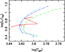
Figure 1: The evolutionary tracks of models with $M=1.50$ $M_{\odot}$ with different $\delta_{\rm ov}$ and $\alpha$. The solid (red) line represents the model track with $\delta_{\rm ov}$ = 0.0; the dashed (green) line represents $\delta_{\rm ov}$ = 1.2; the dash-dotted (blue) line represents $\delta_{\rm ov}$ = 1.4; the dotted (cyan) line represents $\delta_{\rm ov}$ = 1.6. The circles indicate the most likely models for KIC 2837475.

Table 1: The Range of the Parameters of Zero-age MS Models.

Variable	Minimum	Maximum	$\delta$
M/M⊙	1.00	1.60	0.02
$\alpha$	1.65	2.05	0.1
$\delta_{\rm ov}$	0.0	1.8	0.2
$Z_{i}$	0.010	0.050	0.002
$X_{i}$	0.655	0.742	0.002

The adiabatic frequencies of the low-degree p-modes of models are computed by using the Guenther pulsation code (Guenther, 1994). For the modes with a given degree $l$, the frequencies $\nu_{corr}(n)$ corrected from the near-surface effects of a model are calculated by using equation (Kjeldsen et al., 2008)

$$\nu_{corr}(n)=\nu_{mod}(n)+a[\frac{\nu_{mod}(n)}{\nu_{max}}]^{b},$$ (3)

where $b$ is fixed to be 4.9, $a$ is determined from the observed frequencies of the modes with the given $l$ and the adiabatic frequencies of the modes with the degree $l$ of the model by using equations (6) and (10) of Kjeldsen et al. (2008), $\nu_{mod}(n)$ represents the adiabatic frequencies of the model, $\nu_{max}$ is the observed frequency of maximum oscillation power.

3 Observational Constraints

3.1 Non-asteroseismic Observational Constraints

KIC 2837475 is an F5 star (Wright et al., 2003). Its effective temperatures are $6562^{+68}_{-75}$ K (Ammons et al., 2006), $6740\pm 70$ K (Bruntt et al., 2012), or $6462\pm 125$ K (Molenda-Zakowicz et al., 2013). The value of [Fe/H] for KIC 2837475 is $0.21\pm 0.12$ (Ammons et al., 2006), $-0.02\pm 0.06$ (Bruntt et al., 2012), or $-0.06\pm 0.21$ (Molenda-Zakowicz et al., 2013). Combining the value of $(Z/X)_{\odot}=0.023$ given by Grevesse & Sauval (1998), the ratio of surface heavy-element abundance to hydrogen abundance, $(Z/X)_{s}$, can be obtained and is approximately between 0.028 and 0.049 for the [Fe/H] of Ammons et al. (2006), between 0.019 and 0.025 for the [Fe/H] of Bruntt et al. (2012), or between 0.012 and 0.033 for the [Fe/H] of Molenda-Zakowicz et al. (2013). Moreover, its visual magnitude is $8.547\pm 0.013$ mag (Ammons et al., 2006). The bolometric correction can be estimated from the tables of Flower (1996); while extinction is obtained from Ammons et al. (2006). By combining its parallax $\Pi=10.3^{+5.8}_{-5.0}$ mas (Ammons et al., 2006), its luminosity is estimated as approximately $6.0\pm 4.8$ $L_{\odot}$.

For each model, the value of $\chi_{c}^{2}$ is calculated. The function $\chi_{c}^{2}$ is defined as

$$\chi^{2}_{c}=\frac{1}{3}\sum_{i=1}^{3}[\frac{C_{i}^{theo}-C_{i}^{obs}}{\sigma(C_{i}^{obs})}]^{2},$$ (4)

where the quantities $C_{i}^{obs}$ and $C_{i}^{theo}$ are the observed and model values of $T_{\rm eff}$, $L/L_{\odot}$, and $(Z/X)_{s}$, respectively. The observational uncertainty is indicated by $\sigma(C_{i}^{obs})$. In the first step, the models with $\chi_{c}^{2}\leq 1$ are used as candidates for KIC 2837475.

3.2 Asteroseismic Constraints

To find the models that can reproduce the properties of KIC 2837475 , the value of $\chi_{\nu}^{2}$ was computed. The function $\chi_{\nu}^{2}$ is defined as

$$\chi_{\nu}^{2}=\frac{1}{N}\sum_{i=1}^{N}[\frac{\nu_{i}^{theo}-\nu_{i}^{obs}}{\sigma(\nu_{i}^{obs})}]^{2},$$ (5)

where $\nu_{i}^{obs}$ and $\nu_{i}^{theo}$ are the observed and corresponding model eigenfrequencies of the $i$th mode, respectively, and $\mathbf{\sigma(\nu_{i}^{obs})}$ is the observational uncertainty of the $i$th mode. The value of the $N$ is 44 for KIC 2837475. We also calculated the value of $\chi_{\nu_{corr}}^{2}$ of models. The models with $\chi_{c}^{2}\leq 1.0$ and $\chi_{\nu}^{2}$ or $\chi_{\nu_{corr}}^{2}\lesssim 10.0$ are chosen as candidates.

In order to ensure finding the model with the minimum $\chi_{\nu}^{2}$ and the model with the minimum $\chi_{\nu_{corr}}^{2}$, the time-step of the evolution for each track is set as small as possible when the model evolves to the vicinity of the error-box of luminosity and effective temperature in the H-R diagram. This makes the consecutive models have an approximately equal $\chi_{\nu}^{2}$ or $\chi_{\nu_{corr}}^{2}$. The value of $\chi_{\nu_{corr}}^{2}$ of the model with the minimum $\chi_{\nu}^{2}$ is usually not a minimum (see the models Mb1d and Mm2b in Table 2). In some cases, for the consecutive models in a track, the value of the minimum $\chi_{\nu_{corr}}^{2}$ is even larger than that of the minimum $\chi_{\nu}^{2}$ (see the models Mm2b and Mm2d in Table 2). The difference between the age of the model with the minimum $\chi_{\nu}^{2}$ and the age of the model with the minimum $\chi_{\nu_{corr}}^{2}$ is generally several Myr. However, the distributions of ratios $r_{01}$ and $r_{10}$ of the two models are almost the same (see Figure 2), i.e., the interior structures of the two models are almost the same. For a given mass and $\delta_{\rm ov}$, the model with the minimum $\chi_{\nu_{corr}}^{2}$ was chosen as the best model.

Figures 2 and 3 show that the distributions of ratios $r_{01}$ and $r_{10}$ are affected by correction. Kjeldsen et al. (2008) argued that the offset from incorrect modeling of the near-surface layers is independent of $l$. Thus we computed the value of $a$ in equation (3) only from frequencies of radial modes ($l=0$) and then apply it to all modes. In this case, the distributions of ratios $r_{01}$ and $r_{10}$ are not affected by the correction, i.e., the corrected and uncorrected ratios are the same; however, the value of $\chi_{\nu_{corr}}^{2}$ becomes larger (see the value in the parentheses in Table 2). In present work, the $a$ for the modes with degree $l$ is calculated from the observed and model frequencies of the modes with the degree $l$.

3.2.1 The Models with the Effective Temperature and [Fe/H] of Bruntt

For a given mass, the model minimizing $\chi_{\nu_{corr}}^{2}+\chi_{c}^{2}$ is chosen as a candidate for the best-fit model. The fundamental parameters of the models are listed in Table 2, where some consecutive models are listed to state that the value of $\chi_{\nu}^{2}$ of the model with the minimum $\chi_{\nu_{corr}}^{2}$ is not a minimum. The model Mb1b has the minimum $\chi_{\nu_{corr}}^{2}$ and $\chi_{\nu_{corr}}^{2}+\chi_{c}^{2}$, suggesting that Mb1b are the best-fit model.

Table 2: Parameters of Models. The symbol $X_{c}$ indicates the central hydrogen abundance of models. The symbol $r_{cc}$ shows the radius of a convective core of models determined by Schwarzchild criterion; while the $\chi_{\nu_{corr}}^{2}$ represents the chi squared of frequencies corrected from near-surface effects. Models Mb’s have the Effective temperature and [Fe/H] of Bruntt et al. (2012); while models Mm1 to Mm11 have those determined by Molenda-Zakowicz et al. (2013).

Model	$M$	$T_{\rm eff}$	$L$	$R$	age	$Z_{i}$	$(Z/X)_{s}$	$\alpha$	$\delta_{\rm ov}$	$X_{c}$	$r_{cc}$	$\chi_{\nu}^{2}$	$\chi_{\nu_{corr}}^{2}$	$\chi_{c}^{2}$
	($M_{\odot}$)	(K)	($L_{\odot}$)	($R_{\odot}$)	(Gyr)						($R_{\odot}$)
Mb1a	1.30	6821	4.90	1.589	2.036	0.014	0.020	1.95	0.2	0.380	0.125	10.6	5.3 (6.1)a	0.6
Mb1b	1.30	6820	4.90	1.589	2.037	0.014	0.020	1.95	0.2	0.380	0.125	9.0	5.1 (6.0)	0.6
Mb1c	1.30	6820	4.90	1.589	2.038	0.014	0.020	1.95	0.2	0.379	0.125	8.0	5.4 (6.5)	0.6
Mb1d	1.30	6820	4.90	1.589	2.039	0.014	0.020	1.95	0.2	0.379	0.125	7.6	6.5 (7.6)	0.6
Mb1e	1.30	6819	4.90	1.589	2.040	0.014	0.020	1.95	0.2	0.379	0.125	7.8	8.1 (9.3)	0.6
Mb2a	1.32	6786	4.87	1.600	1.717	0.016	0.024	1.95	0.0	0.272	0.111	6.8	7.0 (6.2)	0.3
Mb2b	1.32	6785	4.87	1.600	1.721	0.016	0.024	1.95	0.0	0.271	0.111	6.5	6.3 (6.5)	0.2
Mb2c	1.32	6783	4.88	1.600	1.724	0.016	0.024	1.95	0.0	0.270	0.111	9.2	9.0 (12.9)	0.2
Mb3	1.34	6772	4.89	1.611	1.851	0.018	0.026	1.95	0.2	0.400	0.131	5.8	5.2 (5.7)	0.8
Mm1	1.19	6381	3.66	1.567	3.200	0.014	0.012	1.85	0.2	0.294	0.111	7.1	7.1	0.2
Mm2a	1.21	6529	4.03	1.572	2.553	0.012	0.011	2.05	0.0	0.145	0.095	8.8	15.9	0.2
Mm2b	1.21	6529	4.03	1.572	2.555	0.012	0.011	2.05	0.0	0.145	0.095	7.8	11.6	0.2
Mm2c	1.21	6528	4.03	1.572	2.557	0.012	0.011	2.05	0.0	0.144	0.095	8.4	9.3	0.1
Mm2d	1.21	6528	4.03	1.573	2.558	0.012	0.011	2.05	0.0	0.144	0.093	9.6	8.9	0.1
Mm2e	1.21	6528	4.04	1.573	2.559	0.012	0.011	2.05	0.0	0.143	0.093	12.8	9.4	0.1
Mm3	1.23	6435	3.87	1.585	2.926	0.016	0.015	1.95	0.2	0.311	0.117	6.8	6.7	0.1
Mm4	1.25	6392	3.80	1.592	2.793	0.018	0.016	1.85	0.2	0.334	0.118	7.5	6.9	0.2
Mm5	1.27	6479	4.07	1.603	2.719	0.018	0.018	2.05	0.2	0.325	0.112	7.7	7.1	0.1
Mm6	1.29	6424	3.98	1.611	2.662	0.020	0.020	1.95	0.2	0.341	0.123	7.5	6.9	0.1
Mm7	1.32	6657	4.52	1.600	1.753	0.018	0.027	1.75	0.0	0.293	0.113	8.6	6.4	0.9
Mm8	1.34	6528	4.29	1.622	2.142	0.022	0.032	1.75	0.2	0.392	0.129	9.0	7.4	0.5
Mm9	1.36	6588	4.46	1.622	1.801	0.020	0.029	1.75	0.0	0.311	0.116	7.1	6.8	0.5
Mm10	1.38	6589	4.50	1.629	1.800	0.024	0.035	1.75	0.2	0.427	0.135	6.2	4.7	1.0
Mm11	1.40	6583	4.54	1.641	1.617	0.024	0.035	1.75	0.0	0.344	0.122	6.7	6.4	0.9

^a The corrected frequencies of modes with $l=1$ and $2$ are calculated by using the $a$ that is determined from the frequencies of modes with $l=0$.

However, Figure 4 shows that these models cannot reproduce the observed ratios $r_{01}$ and $r_{10}$. This hints us that the internal structures of these models may be not consistent with that of KIC 2837475.

The effective temperatures of KIC 2837475 determined by Molenda-Zakowicz et al. (2013) and Ammons et al. (2006) are obviously lower than that estimated by Bruntt et al. (2012). Our models with the effective temperature and [Fe/H] of Bruntt et al. (2012) cannot reproduce the observed ratios $r_{01}$ and $r_{10}$. Thus the models with the $T_{\rm eff}$ and [Fe/H] determined by Molenda-Zakowicz et al. (2013) and Ammons et al. (2006) also should be considered.

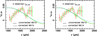
Figure 2: The distributions of ratios $r_{01}$ and $r_{10}$ of models Mb1b and Mb1d as a function of frequency. The uncorrected ratios are calculated from adiabatic frequencies $\nu_{n,l}$ of the models, while the corrected ratios are computed from the corrected frequencies $\nu_{corr}$ of the models.

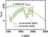
Figure 3: The distributions of corrected and uncorrected ratios $r_{01}$ and $r_{10}$ of model Mb2b.

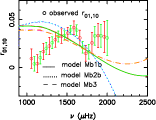
Figure 4: The distributions of the observed and theoretical ratios $r_{01}$ and $r_{10}$ as a function of frequency. The theoretical ratios are calculated from the corrected frequencies $\nu_{corr}$ of models.

3.2.2 The Models with the Effective Temperature and [Fe/H] of Molenda-Zakowicz

Table 2 lists the models with the effective temperature and [Fe/H] of Molenda-Zakowicz et al. (2013). The values of $\chi_{\nu}^{2}$ and $\chi_{\nu_{corr}}^{2}$ of the models are as large as those of models with the effective temperature and [Fe/H] of Bruntt et al. (2012). However, Figure 5 shows that the ratios $r_{01}$ and $r_{10}$ of the models are not in agreement with the observed ones. Our calculatios show that the uncorrected ratios of these models also do not agree with the observed ones, i.e., the internal structures of these models do not match that of KIC 2837475.

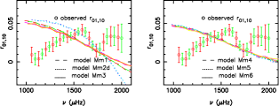
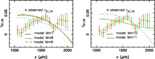
Figure 5: The distributions of the observed and theoretical ratios $r_{01}$ and $r_{10}$ as a function of frequency. The theoretical ratios are calculated from the corrected frequencies $\nu_{corr}$ of models with the effective temperature and [Fe/H] of Molenda-Zakowicz et al. (2013).

The ratios of the models listed in Table 2 decrease with the increase in frequencies. Liu et al. (2014) showed that the ratios of the modes whose inner turning points are located in overshooting region of convective core can exhibit an increase behavior. They also showed that the inner turning point, $r_{t}$, of the mode with a frequency $\nu_{n,1}$ should be estimated by

$$\nu_{n,l}=f_{0}\frac{c(r_{t})}{r_{t}}\frac{\sqrt{l(l+1)}}{2\pi},$$ (6)

where $c(r_{t})$ is the adiabatic sound speed at radius $r_{t}$, the value of the parameter $f_{0}$ is $2.0$.

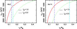
Figure 6: The frequencies of models as a function of inner turning point $r_{t}$ determined by Equation (6). The vertical dash-dotted blue lines show the radius of the convective core determined by Schwarzchild criterion. The vertical dashed cyan lines show the radius of the overshooting region. The solid red lines show the frequencies determined by Equation (6) with $f_{0}=1.0$, while the dotted green lines represent those determined by Equation (6) with $f_{0}=2.0$.

Figure 6 shows the distributions of frequencies $\nu_{n,1}$ of models as a function of inner turning point $r_{t}$ determined by Equation (6). When the value of $f_{0}$ is equal to $2.0$, the modes with $\nu_{n,1}$ less than $2200$ $\mu$Hz do not reach the overshooting region of the convective core of model Mb3. The ratios $r_{01}$ and $r_{10}$ of model Mb3 do not exhibit an increase behavior in the range between 1000 and 2200 $\mu$Hz. When the frequency is larger than 2200 $\mu$Hz, the ratios of model Mb3 exhibit an obvious increase behavior (see Figure 4). Thus the increase behavior of the ratios $r_{01}$ and $r_{10}$ may derive from an effect of the overshooting of convective core.

The radius of overshooting region increase with the increase in $\delta_{\rm ov}$, which leads to the fact that the increase behavior can appear at low frequencies for the star with a large $\delta_{\rm ov}$. Thus, we calculated the models with $\delta_{\rm ov}$ as large as 1.8. With the constraints of the effective temperature and [Fe/H] of Bruntt et al. (2012) and Molenda-Zakowicz et al. (2013), we did not obtain the models that can reproduce the observed frequencies and ratios $r_{01}$ and $r_{10}$.

3.2.3 The Models with the Effective Temperature and [Fe/H] of Ammons

The effective temperature determined by Ammons et al. (2006) is higher than that estimated by Molenda-Zakowicz et al. (2013) but lower than the one determined by Bruntt et al. (2012). Moreover, the value of [Fe/H] estimated by Ammons et al. (2006) is higher than those determined by Bruntt et al. (2012) and Molenda-Zakowicz et al. (2013). We calculated models with the effective temperature and [Fe/H] determined by Ammons et al. (2006). The value of $\delta_{\rm ov}$ of the models with $\chi_{c}^{2}\leq 1.0$ is in the range of 0.0-0.4 and 1.0-1.6. The models with $\delta_{\rm ov}$ between 0.0 and 0.4 can not reproduce the observed ratios $r_{01}$ and $r_{10}$. Table 3 lists the models with the larger $\delta_{\rm ov}$ and a minimum $\chi_{\nu_{corr}}^{2}+\chi_{c}^{2}$ for a given mass and $\delta_{\rm ov}$. The values of $\chi_{\nu_{corr}}^{2}$ of the models are as low as those of models with the effective temperatures of Bruntt et al. (2012) or Molenda-Zakowicz et al. (2013). The value of $\chi_{\nu_{corr}}^{2}$ of the models with $\delta_{\rm ov}$ = 1.4 is generally lower than that of other models. This indicates that the models with $\delta_{\rm ov}$ = 1.4 are better than other models.

Table 3: Parameters of Models with the Effective Temperature and [Fe/H] of Ammons et al. (2006). The symbols have the same meaning as those in Table 2.

Model	$M$	$T_{\rm eff}$	$L$	$R$	age	$Z_{i}$	$(Z/X)_{s}$	$\alpha$	$\delta_{\rm ov}$	$X_{c}$	$r_{cc}$	$\chi_{\nu}^{2}$	$\chi_{\nu_{corr}}^{2}$	$\chi_{c}^{2}$
	($M_{\odot}$)	(K)	($L_{\odot}$)	($R_{\odot}$)	(Gyr)						($R_{\odot}$)
Ma1	1.44	6633	4.78	1.660	3.194	0.028	0.039	1.95	1.2	0.575	0.159	16.7	8.3	0.4
Ma2	1.44	6674	4.88	1.656	3.320	0.028	0.039	1.95	1.4	0.584	0.160	17.4	6.9	0.9
Ma3	1.44	6530	4.54	1.667	4.202	0.036	0.051	1.95	1.6	0.571	0.161	11.0	7.8	0.5
Ma4	1.46	6473	4.39	1.667	2.850	0.032	0.045	1.75	1.0	0.575	0.158	18.1	8.1	0.7
Ma5	1.46	6510	4.47	1.663	2.980	0.032	0.045	1.75	1.2	0.587	0.159	15.3	7.2	0.3
Ma6	1.46	6614	4.78	1.667	3.353	0.032	0.045	1.95	1.4	0.582	0.162	12.2	6.9	0.3
Ma7	1.46	6494	4.44	1.667	3.547	0.036	0.051	1.75	1.6	0.591	0.163	8.8	7.2	0.8
Ma8	1.48	6555	4.62	1.667	2.495	0.030	0.042	1.75	1.0	0.590	0.159	17.4	6.9	0.1
Ma9	1.48	6607	4.81	1.675	2.984	0.032	0.045	1.95	1.2	0.582	0.162	13.5	7.6	0.3
Ma10	1.48	6489	4.46	1.675	3.148	0.036	0.051	1.75	1.4	0.594	0.164	13.4	5.8	0.8
Ma11	1.48	6638	4.88	1.675	3.379	0.034	0.048	1.95	1.6	0.591	0.165	7.2	6.3	0.7
Ma12	1.50	6561	4.67	1.675	2.194	0.034	0.048	1.75	1.0	0.589	0.163	19.7	5.7	0.3
Ma13	1.50	6547	4.63	1.675	2.417	0.036	0.051	1.75	1.2	0.594	0.165	17.2	5.4	0.5
Ma14	1.50	6579	4.71	1.671	2.523	0.036	0.051	1.75	1.4	0.600	0.166	17.0	5.5	0.5
Ma15	1.50	6610	4.78	1.671	2.626	0.036	0.051	1.75	1.6	0.604	0.167	17.1	5.9	0.7
Ma16	1.52	6543	4.67	1.683	2.248	0.034	0.048	1.75	1.0	0.599	0.164	16.6	5.6	0.3
Ma17	1.52	6594	4.86	1.690	2.731	0.036	0.051	1.95	1.2	0.589	0.167	9.5	6.6	0.5
Ma18	1.52	6628	4.94	1.687	2.841	0.036	0.051	1.95	1.4	0.597	0.166	7.8	5.3	0.7
Ma19	1.52	6592	4.78	1.679	2.690	0.036	0.051	1.75	1.6	0.614	0.167	16.9	5.0	0.5
Ma20	1.54	6639	5.01	1.694	2.268	0.034	0.048	1.95	1.0	0.593	0.166	9.5	6.3	0.7
Ma21	1.54	6628	4.98	1.694	2.496	0.036	0.051	1.95	1.2	0.598	0.167	8.1	5.7	0.7
Ma22	1.54	6595	4.83	1.687	2.351	0.036	0.050	1.75	1.4	0.618	0.168	16.6	5.5	0.5
Ma23	1.54	6625	4.90	1.683	2.446	0.036	0.050	1.75	1.6	0.622	0.169	19.0	5.8	0.7
Ma24	1.56	6637	5.04	1.702	2.137	0.036	0.051	1.95	1.0	0.597	0.167	9.6	5.8	0.8
Ma25	1.56	6608	4.90	1.690	1.998	0.036	0.051	1.75	1.2	0.620	0.168	17.8	5.5	0.6
Ma26	1.56	6636	4.97	1.687	2.091	0.036	0.051	1.75	1.4	0.625	0.169	18.9	6.6	0.8

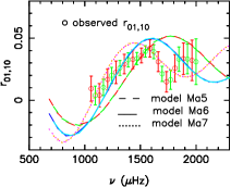
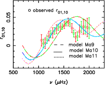
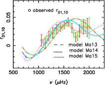
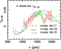
Figure 7: The distributions of the observed and theoretical ratios $r_{01}$ and $r_{10}$ as a function of frequency. The theoretical ratios are calculated from the corrected frequencies $\nu_{corr}$ of models with the effective temperature and [Fe/H] of Ammons et al. (2006).

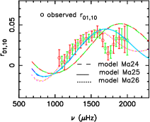
Figure 8: The distributions of ratios $r_{01}$ and $r_{10}$ calculated from the corrected frequencies of models Ma24, Ma25, and Ma26.

Figures 7 and 8 show the distributions of ratios $r_{01}$ and $r_{10}$ of the models listed in Table 3 as a function of frequency, which clearly show that the observed ratios can be reproduced by the models with mass between about 1.46 and 1.56 $M_{\odot}$ and $\delta_{\rm ov}$ between 1.2 and 1.6. This indicates that KIC 2837475 may has a very thick overshooting region of convective core.

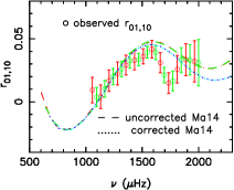
Figure 9: The distribution of corrected and uncorrected ratios $r_{01}$ and $r_{10}$ of model Ma14 as a function of frequency.

The distributions of ratios $r_{01}$ and $r_{10}$ can be affected by the correction for the effect of near-surface layers. Thus we computed the ratios of uncorrected frequencies of the models listed in Table 3. Figure 9 shows that the difference between the uncorrected and corrected ratios mainly occurs at high frequency. The distribution of the corrected ratios is similar to that of uncorrected ones for these models. Therefore, the increase behavior of the ratios of the models is uncorrelated with the effect of the correction. It derives from an effect of the overshooting of convective core. Even using the uncorrected ratios or the ratios of models with the minimum $\chi_{\nu}^{2}$, our results are not changed.

3.3 Fitting Curves of the Observed and Theoretical Ratios

Yang et al. (2015) suggested using equation

$$r_{10}(\nu_{n,1})=\frac{2A\nu_{0}}{2\pi^{2}(\nu^{2}_{0}-\nu^{2}_{n,1})}\sin(2\pi\frac{\nu_{n,1}}{\nu_{0}})+B_{0},$$ (7)

or

$$r_{10}(\nu_{n,1})=\frac{2A\nu_{n,1}}{2\pi^{2}(\nu^{2}_{0}-\nu^{2}_{n,1})}\sin(2\pi\frac{\nu_{n,1}}{\nu_{0}})+B_{0},$$ (8)

to describe the ratios $r_{01}$ and $r_{10}$ affected by the overshooting of the convective core of stars, where the $A$ is a free parameter, the $\nu_{0}$ is the frequency of the mode whose inner turning point is located on the boundary between the radiative region and the overshooting region of convective core, the $B_{0}$ is the $r_{10}$ at $3\nu_{0}/2$. The value of $r_{10}(\nu_{n,1})$ decreases with frequency $\nu_{n,1}$ when the frequency is less than $\nu_{0}$ but increases with frequency in the range of approximately $\nu_{0}$ and $7\nu_{0}/4$, and has a maximum at about $7\nu_{0}/4$. The distributions of ratios $r_{01}$ and $r_{10}$ of KIC 2837475 provide a good opportunity for testing the formulae.

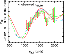
Figure 10: The distribution of $r_{10}$ as a function of $\nu_{n,1}$. The dashed green line represents the ratio computed by using equation (7) with $A=50\pi$, $\nu_{0}=900$ $\mu$Hz and $B_{0}=0.032$. The solid red line shows the ratio calculated by using equation (8) with $A=50\pi$, $\nu_{0}=900$ $\mu$Hz and $B_{0}=0.032$. The dotted lines represent the ratios of model Ma14.

The observed ratios of KIC 2837475 has a maximum at about $1580$ $\mu$Hz. Thus the value of $\nu_{0}$ is approximately $900$ $\mu$Hz. The value of the observed $r_{10}$ of KIC 2837475 is about 0.032 at 1390 $\mu$Hz. Yang et al. (2015) showed that the value of $A$ is $50\pi$ for KIC 11081729 and HD 49933. With $A=50\pi$, $\nu_{0}=900$ $\mu$Hz, and $B_{0}=0.032$, we calculated $r_{10}$ for KIC 2837475 using Equations (7) and (8). Figure 10 represents the $r_{10}$ as a function of $\nu_{n,1}$. The $r_{10}$ determined by Equation (7) is more consistent with the observed ratios than that determined by Equation (8). However, when the frequency $\nu_{n,1}$ is larger than $3\nu_{0}/2$, the $r_{10}$ determined by Equation (8) is in better agreement with the ratios of model Ma14 than that determined by Equation (7). The observed and theoretical ratios can be well reproduced by Equations (7) and (8). This further states that the increase behavior in the ratios of KIC 2837475 arises from the effect of the overshooting of convective core.

3.4 Comparisons with Previous Models

In the calculations, the effects of the overshooting of the convective core were included that were not considered by Metcalfe et al. (2014) in their models. Moreover, the evolutions of models with a mass larger than $1.30$ $M_{\odot}$ were computed without diffusion, while Metcalfe et al. (2014) considered the case with helium diffusion. The diffusion of helium and heavy elements of Thoul et al. (1994) could produce the almost metal-free and pure-hydrogen models in the evolutions of models with a mass larger than $1.30$ $M_{\odot}$ when the value of the mixing-length parameter is small. For example, when the value of $\alpha$ is $1.75$, the value of the surface metallicity of the model with $M=1.50$ and $Z_{i}=0.03$ can decrease to 0.003. Thus we did not consider the diffusion in the evolutions of models with a mass larger than 1.30 $M_{\odot}$.

The mass of KIC 2837475 determined by Metcalfe et al. (2014) is $1.39\pm 0.06$ $M_{\odot}$, which is consistent with the mass of the models with the effective temperature and [Fe/H] of Molenda-Zakowicz et al. (2013). However, the models cannot reproduce the observed ratios. The mass of the models with the effective temperature and [Fe/H] of Ammons et al. (2006) is obviously higher than that determined by Metcalfe et al. (2014). The value of the large separation ($\Delta\nu$) and the frequency of maximum seismic amplitude ($\nu_{max}$) is $76$ and $1522$ $\mu$Hz (Appourchaux et al., 2012) for KIC 2837475, respectively. Using equation

$$M=(\frac{\Delta\nu}{\Delta\nu_{\odot}})^{-4}(\frac{\nu_{max}}{\nu_{max,\odot}})^{3}(\frac{T_{\rm eff}}{T_{\rm eff,\odot}})^{3/2}M_{\odot},$$ (9)

we estimated the mass of KIC 2837475. The value of the mass is $1.493$ $M_{\odot}$ for the effective temperature of $6562$ K of Ammons et al. (2006), $1.554$ $M_{\odot}$ for the effective temperature of $6740$ K of Bruntt et al. (2012), and $1.460$ $M_{\odot}$ for the effective temperature of $6462$ K of Molenda-Zakowicz et al. (2013). Only the mass of the models with the effective temperature and [Fe/H] of Ammons et al. (2006) is consistent with that estimated by Equation (9).

4 DISCUSSION AND SUMMARY

4.1 Discussion

The values of the acoustic depth $\tau_{HeIIZ}$ and $\tau_{BCZ}$ (Mazumdar et al., 2014) of model Ma14 are about 740 and 3770 $s$, respectively. The changes caused by the glitch at the base of the convective envelope or the second helium ionization zone have a periodicity of twice the depth of the corresponding glitch (Mazumdar et al., 2014). For the model Ma14, the periods are 1480 and 7540 $s$ which are corresponding to the frequencies of 675.7 and 132.6 $\mu$Hz, respectively. The ratios $r_{01}$ and $r_{10}$ of KIC 2837475 almost linearly increase in the range of approximately 1050 and 1600 $\mu$Hz. Thus the changes in the ratios could not derive from the effects of the glitch at the base of the convective envelope or the second helium ionization zone.

Figure 6 shows that the modes with a frequency larger than about 760 $\mu$Hz penetrate into the overshooting region for model Ma14. Figure 10 shows that an obvious increase behavior of ratios of model Ma14 occurs at the frequencies larger than about 850 $\mu$Hz. In addition, Figure 7 shows that the values of the frequencies of the minimum and maximum $r_{10}$ decrease with the increase in $\delta_{\rm ov}$. The increase in $\delta_{\rm ov}$ leads to the increase in the radius of overshooting region, which results in the decrease in frequency $\nu_{0}$, i.e., the location of the increase ratios moves to low frequencies with the increase in $\delta_{\rm ov}$. Therefore, the increase behavior of the ratios is related to the effects of overshooting of convective core.

The minimum of the Equations (7) and (8) does not occur at $\nu_{0}$. For example, when the value of $\nu_{0}$ is 900 $\mu$Hz, the minimum of the Equation (7) occurs at 866 $\mu$Hz; but the minimum of the Equation (8) occurs at 934 $\mu$Hz. This leads to the difference between the results of Equations (7) and (8) at $\nu_{n,1}<3\nu_{0}/2$. The minimum of the ratios of model Ma14 is located at about 850 $\mu$Hz. Thus the results calculated by Equation (7) is more consistent with theoretical ratios when frequencies are less than $3\nu_{0}/2$.

The values of parameters $A$, $\nu_{0}$, and $B_{0}$ can be estimated from the observed $\nu_{n,1}$ and $r_{10}$ and are $34\pm 10$ $\pi$, $900\pm 35$ $\mu$Hz, and $0.030\pm 0.002$ respectively for Equation (7), $23\pm 7$ $\pi$, $913\pm 36$ $\mu$Hz, and $0.030\pm 0.002$ respectively for Equation (8). The values of $\nu_{0}$ and $B_{0}$ determined by using the observed $r_{10}$ and Equation (7) are consistent with those determined by using the observed $r_{10}$ and Equation (8). However, the values of $A$ have an obvious difference. The Equations (7) and (8) have a minimum at about $\nu_{0}$ and a maximum at around $7\nu_{0}/4$. The observed ratios of KIC 2837475 have not the minimum. Thus the observed ratios are not suitable to determine the value of $A$.

Radiative levitation can lead to overabundances of Cr, Mn, Fe, and Ni at the surface of stars with a mass larger than $1.30$ $M_{\odot}$ (Turcotte et al., 1998). It is difficult to compute the radiative levitation effects in the evolutions of a large sample of models because of numerical instabilities (Turcotte et al., 1998). Thus the effects of radiative accelerations are not considered in our models with a mass larger than $1.30$ $M_{\odot}$.

Tables 2 and 3 clearly show that the value of the mass of the obtained models is dependent on the effective temperature and [Fe/H]. Due to the fact that the models with the effective temperature and [Fe/H] of Bruntt et al. (2012) or Molenda-Zakowicz et al. (2013) can not reproduce the observed ratios $r_{01}$ and $r_{10}$, only the models with the effective temperature and [Fe/H] of Ammons et al. (2006) were used to estimate the mass, radius, and age of KIC 2837475.

A large $\delta_{\rm ov}$ means that an efficient mixing exists in interior of stars. The mass of Procyon is $1.497\pm 0.037$ $M_{\odot}$. The mass of our models for KIC 2837475 is in the range of approximately 1.46 and 1.56 $M_{\odot}$. Moreover, there is the phenomenon of the double or extended MS turnoffs in the color-magnitude diagram of intermediate-age star clusters in the Large Magellanic Cloud (Mackey & Broby Nielsen, 2007; Milone et al., 2009; Goudfrooij et al., 2009). The mass of the MS-turnoff stars of the clusters is around 1.5 $M_{\odot}$ (Yang et al., 2011b, 2013). Yang et al. (2013) showed that rapid rotation and extra mixing caused by rotation can be used to explain the extended MS turnoffs. The surface rotation period of KIC 2837475 is about 3.7 days (García et al., 2014; McQuillan et al., 2014). Rotation can lead to an increase in the convective core, which depends on the efficiency of rotational mixing and rotation rate (Maeder, 1987; Yang et al., 2013). Furthermore, the extra mixing caused by rotation can mimic the effect of the overshooting to a certain degree. This hints us that the large $\delta_{\rm ov}$ in KIC 2837475 may be related to rotation. The large amount of overshoot may be the consequence of current inaccuracies in the physical models that include many approximations. The “large $\delta_{\rm ov}$” of KIC 2837475 may be not an exceptional case in stars.

4.2 Summary

The calculations show that the observed ratios $r_{01}$ and $r_{10}$ of KIC 2837475 cannot be reproduced by the models with $\delta_{\rm ov}$ $<1.2$. The value of $\delta_{\rm ov}$ is restricted between approximately 1.2 and 1.6 for KIC 2837475, which is very close to that determined by Guenther et al. (2014) for Procyon. The effects of overshooting of the convective core can lead to an increase behavior of ratios $r_{01}$ and $r_{10}$ of the p-modes whose inner turning points are located in overshooting region. For KIC 2837475, the inner turning points of p-modes with $l=1$ are located in the region of overshooting of the convective core. The increase behaviors of the ratios $r_{01}$ and $r_{10}$ of KIC 2837475 result from the effects of overshooting of the convective core. KIC 2837475 shows the existence of large $\delta_{\rm ov}$ and also confirms that the increase behavior of ratios $r_{01}$ and $r_{10}$ derives from the direct effects of overshooting of the convective core.

The increase in $\delta_{\rm ov}$ can lead to the increase in the radius of overshooting region, which results in the fact that the low-frequency modes can penetrate into the overshooting region. the ratios $r_{01}$ and $r_{10}$ of p-modes whose inner turning points are located in the overshooting region can exhibit an increase behavior. Thus the distributions of the ratios $r_{01}$ and $r_{10}$ are sensitive to $\delta_{\rm ov}$. The distributions of the observed and theoretical ratios $r_{01}$ and $r_{10}$ of KIC 2837475 are reproduced well by the equations of Yang et al. (2015), which also indicates that the increase behavior of the ratios arises from the effects of overshooting of the convective core. For the evolutions without the effects of diffusion, with the constraints of Ammons et al. (2006) spectroscopic results and the observed $r_{01}$ and $r_{10}$, the observational constraints favor a star with $M=1.490\pm 0.018$ $M_{\odot}$, $R=1.67\pm 0.01$ $R_{\odot}$, age $=2.8\pm 0.4$ Gyr, and $1.2\lesssim$ $\delta_{\rm ov}$ $\lesssim 1.6$ for KIC 2837475, where the uncertainty indicates the 68% level confidence interval determined by probability distribution function.

References

- Alexander & Ferguson (1994) Alexander, D. R., Ferguson, J. W., 1994, ApJ, 437, 879
- Ammons et al. (2006) Ammons, S. M., Robinson, S. E., Strader, J., Laughlin, G., Fischer, D., & Wolf, A., 2006, ApJ, 638, 1004
- Appourchaux et al. (2008) Appourchaux, T. et al., 2008, A&A, 488, 705
- Appourchaux et al. (2012) Appourchaux, T. et al., 2012, A&A, 543, A54
- Appourchaux et al. (2014) Appourchaux, T. et al., 2014, A&A, 566, A20
- Bruntt et al. (2012) Bruntt, H. et al., 2012, MNRAS, 423, 122
- Chaplin et al. (2014) Chaplin, W. J. et al., 2014, ApJs, 210, 1
- Christensen-Dalsgaard & Houdek (2010) Christensen-Dalsgaard, J., & Houdek, G., 2010, Ap&SS, 328, 51
- Cunha & Metcalfe (2007) Cunha, M. S., & Metcalfe, T. S., 2007, ApJ, 666, 413
- Deheuvels et al. (2010) Deheuvels, S. et al., 2010, A&A, 515, A87
- Demarque et al. (1994) Demarque, P., Sarajedini, A., Guo, X.-J., 1994, ApJ, 426, 165
- De Meulenaer et al. (2010) De Meulenaer, P. et al., 2010, A&A, 523, A54
- Eggenberger et al. (2005) Eggenberger, P., Carrier, F., & Bouchy, F., 2005, NewA, 10, 195
- Flower (1996) Flower, P. J., 1996, ApJ, 469, 355
- García et al. (2014) García, R. A. et al., 2014, A&A, 572, A34,
- Goudfrooij et al. (2009) Goudfrooij, P., Puzia, T. H., Kozhurina-Platais, V., & Chandar, R., 2009, AJ, 137, 4988
- Grevesse & Sauval (1998) Grevesse, N., & Sauval, A. J., 1998, in Solar Composition and Its Evolution, ed. C. Frhlich et al. (Dordrecht: Kluwer), 161
- Guenther (1994) Guenther, D. B., 1994, ApJ, 422, 400
- Guenther et al. (2014) Guenther, D. B., Demarque, P., & Gruberbauer, M., 2014, ApJ, 787, 164
- Iglesias & Rogers (1996) Iglesias, C., Rogers, F. J., 1996, ApJ, 464, 943
- Kjeldsen et al. (2008) Kjeldsen, H., Bedding, T. R., & Christensen-Dalsgaard, J., 2008, ApJL, 683, L175
- Liu et al. (2014) Liu, Z. et al., 2014, ApJ, 780, 152
- Mackey & Broby Nielsen (2007) Mackey, A. D., & Broby Nielsen, P., 2007, MNRAS, 379, 151
- Maeder (1987) Maeder, A., 1987, A&A, 178, 159
- Mazumdar et al. (2006) Mazumdar, A., Basu, S., Collier, B. L., & Demarque, P., 2006, MNRAS, 372, 949
- Mazumdar et al. (2014) Mazumdar, A. et al., 2014, ApJ, 782, 18
- McQuillan et al. (2014) McQuillan, A., Mazeh, T., Aigrain, S., 2014, ApJs, 211, 24
- Metcalfe et al. (2014) Metcalfe, T. S. et al., 2014, ApJs, 214, 27
- Milone et al. (2009) Milone, A. P., Bedin, L. R., Piotto, G., & Anderson, J., 2009, A&A, 497, 755
- Molenda-Zakowicz et al. (2013) Molenda-Zakowicz, J. et al., 2013, MNRAS, 434, 1422
- Montalbán et al. (2013) Montalbán, J., Miglio, A., Noels, A., Dupret, M. A., Scuflaire, R., & Ventura, P., 2013, ApJ, 766, 118
- Pinsonneault et al. (1989) Pinsonneault, M. H., Kawaler, S. D., Sofia, S., & Demarqure, P., 1989, ApJ, 338, 424
- Prather & Demarque (1974) Prather, M. J., & Demarque, P., 1974, ApJ, 193, 109
- Rogers & Nayfonov (2002) Rogers, F. J., & Nayfonov, A., 2002, ApJ, 576, 1064
- Roxburgh & Vorontsov (2003) Roxburgh, I. W., & Vorontsov, S. V., 2003, A&A, 411, 215
- Schrder et al. (1997) Schrder K. P., Pols O. R., Eggleton P. P., 1997, MNRAS, 285, 696
- Silva Aguirre et al. (2011) Silva Aguirre, V., Ballot, J., Serenelli, A. M., & Weiss, A., 2011, A&A, 529, A63
- Silva Aguirre et al. (2013) Silva Aguirre, V. et al., 2013, ApJ, 769, 141
- Stello et al. (2009) Stello, D., Chaplin, W. J., Basu, S., Elsworth, Y., & Bedding, T. R., 2009, MNRAS, 400, L80
- Tian et al. (2014) Tian, Z. J. et al., 2014, MNRAS, 445, 2999
- Thoul et al. (1994) Thoul, A. A., Bahcall, J. N., Loeb, A., 1994, ApJ, 421, 828
- Turcotte et al. (1998) Turcotte, S., Richer, J., & Michaud, G., 1998,ApJ, 504, 559
- Wright et al. (2003) Wright, C. O., Egan, M. P., Kraemer, K. E., Price, S. D., 2003, AJ, 125, 359
- Yang & Bi (2007a) Yang, W., & Bi, S., 2007a, ApJL, 658, L67
- Yang & Bi (2007b) Yang, W., & Bi, S., 2007b, A&A, 472, 571
- Yang et al. (2015) Yang, W., Bi, S., Li, T., Tian, Z., 2015, ApJ, submitted, arXiv:1508.00955
- Yang et al. (2013) Yang, W., Bi, S. Meng, X., & Liu, Z., 2013, ApJ, 776, 112
- Yang et al. (2011a) Yang, W., Li, Z., & Meng, X., Bi, S., 2011a, MNRAS, 414, 1769
- Yang et al. (2011b) Yang, W., Meng, X., Bi, S., Tian, Z., Li, T., & Liu, K., 2011b, ApJL, 731, L37
- Yang et al. (2012) Yang, W., Meng, X., Bi, S., Tian, Z., Liu, K., Li, T., Li, Z., 2012, MNRAS, 422, 1552
- Yang et al. (2010) Yang, W., Meng, X., & Li, Z., 2010, MNRAS, 409, 873