Optical and Radio Variability of BL Lacertae

Abstract

We observed the prototype blazar, BL Lacertae, extensively in optical and radio bands during an active phase in the period 2010–2013 when the source showed several prominent outbursts. We searched for possible correlations and time lags between the optical and radio band flux variations using multifrequency data to learn about the mechanisms producing variability.

During an active phase of BL Lacertae, we searched for possible correlations and time lags between multifrequency light curves of several optical and radio bands. We tried to estimate any possible variability timescales and inter-band lags in these bands. We performed optical observations in B, V, R and I bands from seven telescopes in Bulgaria, Georgia, Greece and India and obtained radio data at 36.8, 22.2, 14.5, 8 and 4.8 GHz frequencies from three telescopes in Ukraine, Finland and USA. Significant cross-correlations between optical and radio bands are found in our observations with a delay of cm-fluxes with respect to optical ones of $\sim$250 days. The optical and radio light curves do not show any significant timescales of variability. BL Lacertae showed many optical ‘mini-flares’ on short time-scales. Variations on longer term timescales are mildly chromatic with superposition of many strong optical outbursts. In radio bands, the amplitude of variability is frequency dependent. Flux variations at higher radio frequencies lead the lower frequencies by days or weeks. The optical variations are consistent with being dominated by a geometric scenario where a region of emitting plasma moves along a helical path in a relativistic jet. The frequency dependence of the variability amplitude supports an origin of the observed variations intrinsic to the source.

1 Introduction

BL Lacertae is the prototype of the BL Lac class of active galactic nuclei and has been observed in optical bands from a long time. It is highly variable in all wavelengths ranging from radio to $\gamma$-ray bands (Raiteri et al. 2013 and references therein). This source is a favourite target of multi-wavelength campaigns of WEBT/GASP and is well known for its intense optical variability on all accessible time-scales (Raiteri et al. 2009; Villata et al. 2009; Raiteri et al. 2010, 2011, 2013 and references therein).

Raiteri et al. (2009) presented the multi-wavelength data (from radio to X-rays) of BL Lac of their 2007–2008 Whole Earth Blazar Telescope (WEBT) campaign and fitted the SEDs by an inhomogeneous, rotating helical jet model (Villata & Raiteri 1999; Ostorero et al. 2004; Raiteri et al. 2003) which includes synchrotron plus self-compton emission from a helical jet plus a thermal component from the accretion disc. Larionov et al. (2010) studied the behaviour of BL Lacertae optical flux and colour variability and suggested the variability to be mostly caused by changes of the Doppler factor. Raiteri et al. (2010) studied the broad band emission and variability properties of the BL Lacertae during the period 2008–2009 and argued for a jet geometry where changes in our viewing angle to the emitting regions plays an important role in the source’s multiwavelength behaviour. Within the optical bands, a bluer when brighter chromatic trend was detected in BL Lacertae in previous studies (e.g., Villata et al. 2002; Gu et al. 2006; Gaur et al. 2012a; Agarwal & Gupta 2015).

Connection of optical and radio light curves has shown significant correlations, with a radio time delay of about 100 days, which can explained by the geometric effects in a rotating helical path in a curved jet (Villata et al. 2009). This source is known to vary on different timescales, with the usual abbreviations being IDV (intra-day variations – within one night) to STV (short-term variations – on timescales of days to weeks) to LTV (long-term variations – on timescales of months and years) (Gupta et al. 2004). It has been claimed to exhibit periodicities in its radio flux variations with a long term component of P $\sim$8 years (Hagen-Thorn et al. 1997; Villata et al. 2004; Villata et al. 2009). Raiteri et al. (2013) collected exceptional optical sampling by the GLAST-AGILE Support Program of the WEBT during the outburst period of the BL Lacertae (2008–2012) and performed cross-correlations between the optical–$\gamma$-ray and X-ray–mm wavelengths which suggest that the region producing the mm and X-ray radiation is located downstream from the optical and $\gamma$-ray emitting zone in the jet. They found a significant cross-correlation between the optical and mm flux densities with a time lag of 120-150 days. Recently, Guo et al. (2015) analysed the historical light curves of optical and radio bands from 1968–2014 to find possible periods of $\sim$1.26 and $\sim$7.50 years, respectively.

The search for correlations between different bands provides crutial information for the emission mechanism and since the radio and optical bands are both attibuted to the synchrotron emission from the relativistic electrons in the jets of blazars, they are of particular importance. A key motivation of this study is to investigate the correlated optical and radio variability (at cm wavelengths) of BL Lacertae during its active state in 2010–2013 when the source showed multiple outbursts in both of these bands. Also, we studied the nature of short- and long-term variability in optical bands as well as variability behaviour in radio bands and their possible variability timescales. Over the course of 3 years, we performed quasi-simultaneous optical multi-band photometric data from seven telescopes in Bulgaria, Greece, Georgia and India on 192 nights. The radio data were observed from Ukraine, Finland and USA at five frequencies, 36.8, 22.2, 14.5, 8 and 4.8 GHz on 302 nights.

The paper is presented as follows: in section 2, we briefly describe the observations and data reductions. We present our results in section 3 and section 4 includes a discussion and our conclusions.

2 Observations and data reduction

2.1 Optical Data

Observations of BL Lacertae started on June 2010 and ran through July 2013 and the entire timeline of the observational period, along with the long-term light curves are shown in Figure 1. The observations were carried out at seven telescopes in Bulgaria, Greece, Georgia and India. The telescopes and cameras that were involved in these observations are described in detail in Gaur et al. (2012b).

Most of the observations were made at the 50/70 cm Schmidt and the 2m Ritchey–Chretien telescopes at Rozhen National Astronomical Observatory, Bulgaria, the 60 cm Cassegrain Telescope at Astronomical Observatory Belogradchik, Bulgaria, and the 1.3m Skinakas Observatory, Crete, Greece during the period June 2010 and July 2013. Instrumental magnitudes and the comparison stars were extracted using the MIDAS package DAOPHOT with an aperture radii of 4 arcsec. We used data of 50 days of observations from Rozhen 50/70 cm telescope, 35 from 2m Rozhen, 72 from Belogradchik and 25 from Skinakas Observatory.

The calibration of the source magnitude was performed with respect to the comparison stars B, C and H (Fiorucci & Tosti 1996). The host galaxy of BL Lacertae is relatively very bright, hence, in order to remove its contribution from the observed magnitudes, we first dereddened the data using the Galactic extinction coefficients of Schlegel et al. (1998) and then subtracted the host galaxy contribution from the observed magnitudes corresponding to that aperture radii (using Nilsson et al. 2007) in order to avoid its contamination in the extraction of colour indicies.

Observations of BL Lacertae on 10, 11, 12 and 14 June 2010 were carried out using the 1.04m Sampurnanand telescope located at Nainital, India. Pre-processing of the raw data which includes bias subtraction, flat-fielding and cosmic ray removal was performed using standard data reduction procedures in IRAF. Reduction of the image frames was done using DAOPHOT II. Aperture photometry was carried out using four concentric aperture radii, i.e., $\sim$ 1 $\times$ FWHM, 2 $\times$ FWHM, 3 $\times$ FWHM and 4 $\times$ FWHM. We found that aperture radii of 2 $\times$ FWHM always provides the best S/N, so we adopted that aperture for our final results.

The observations at the Abastumani Observatory were conducted on 9, 11, 12, 14, 15 and 16 December 2010 at the 70-cm meniscus telescope (f/3). These measurements were made with an Apogee CCD camera Ap6E (1K $\times$ 1K, 24 micron square pixels) through a Cousins R filter with exposures of 60–120 sec. Pre-processing of the raw data is done by IRAF. Reduction of the image frames were done using DAOPHOT II. An aperture radius of 5 arcsec was used for data analysis.

Finally, we also include the published R band data from GASP/WEBT observations (Raiteri et al. 2013) during this period 2010–2013 where magnitudes are extracted for the BL Lac and the standard stars using an aperture radius of 8 arcsec. Hence, we dereddened the data using the Galactic extinction coefficient of Schlegel et al. (1998) and then removed the host galaxy contribution as described above. All the optical data are presented in the top panel of Figure 1.

2.2 Radio Data

The observations were carried out with the 22-m radio telescope (RT-22) at the Crimean Astronomical Observatory (CrAO). For our measurements, we used two similar Dicke switched radiometers of 22.2 and 36.8 GHz. The antenna temperatures from sources were measured by the standard on–on method. Before measuring the intensity, we determined the source position by scanning. The radio telescope was then pointed at the source alternately by the principal and reference (arbitrary) beam lobes formed during beam modulation and having mutually orthogonal polarizations. The antenna temperature from a source was defined as the difference between the radiometer responses averaged over 30 s at two different antenna positions. Depending on the intensity of the emission from sources, we made a series of 6–20 measurements and then calculated the mean signal intensity and estimated the rms error of the mean.

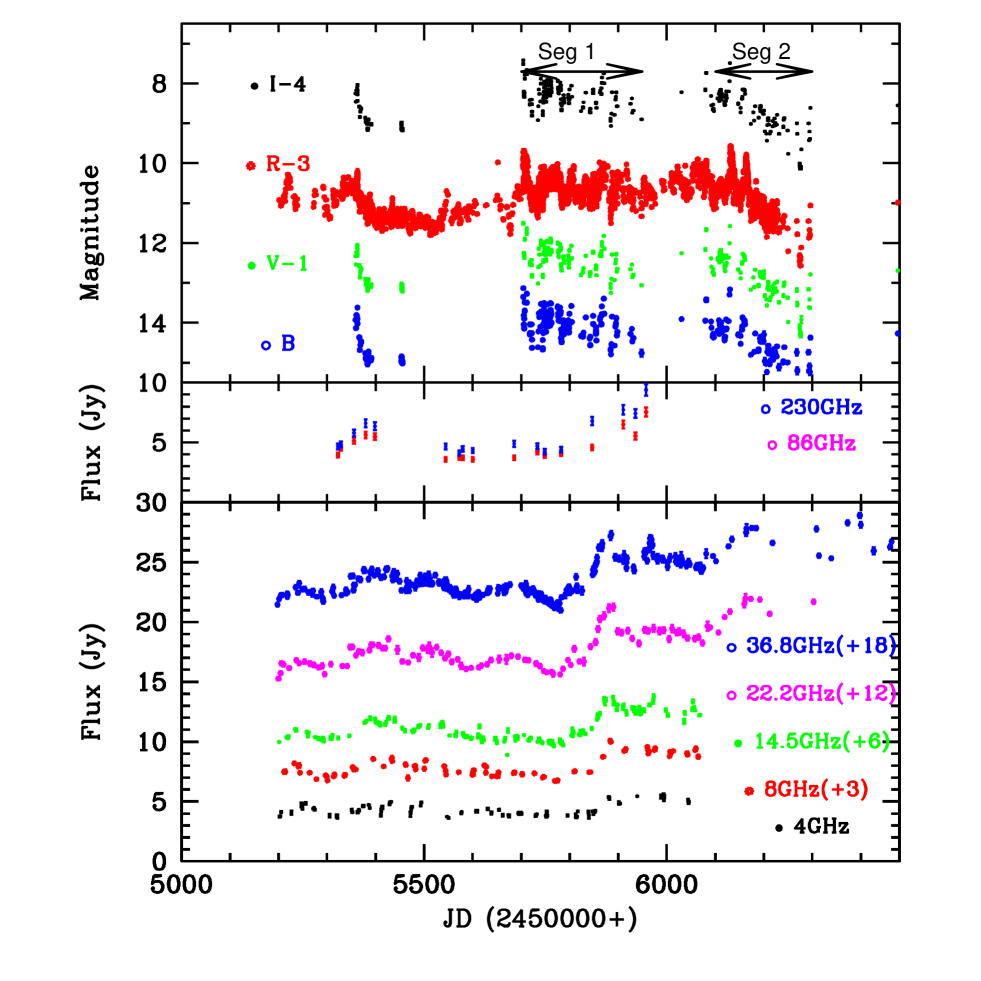
Figure 1: The entire timeline of the observations in optical B, V, R and I bands (upper panel), the radio bands at 230 and 86 GHz (middle panel) and at 36.8 (and 37.0), 22.2, 14.5, 8.0 and 4.8 GHz frequencies (lower panel). The individual light curves and their offsets are labeled.

The gain of the receiver was monitored using a noise generator every 2 to 3 hours. The orthogonal polarization of the lobes allowed us to measure the total intensity of the emission from sources, irrespective of the polarization of this emission. Absorption in the Earth’s atmosphere was taken into account by using atmospheric scans made every 3 to 4 hours. The errors of the calculated optical depths are believed to be less than 10%. The errors of the measured flux densities include the uncertainties of: (1) the detected mean value of the antenna temperature of the sources; (2) the calibration source measurements; (3) the noise generator level measurement; and (4) the atmosphere attenuation corrections. The main contributions to the quoted errors come from the first two terms. The flux density scale of observations was calibrated using DR 21, 3C 274, Jupiter and Saturn.

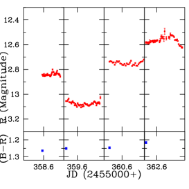
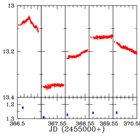
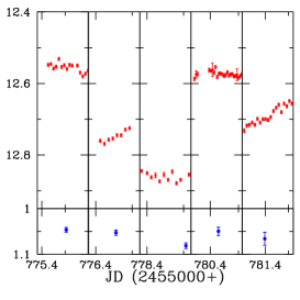
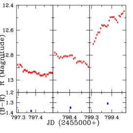
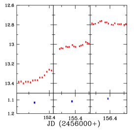
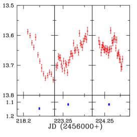
Figure 2: Short-term variability data for BL Lacertae in the R band (in upper panel portions) for each labeled date and the respective average colour indices (B-R) for those nights (lower portions).

Observations at 37.0 GHz were made with the 14 m radio telescope of Aalto University’s Metsähovi Radio Observatory in Finland. Data obtained at Metsähovi and RT-22 were combined in a single array to supplement each other. The flux density scale is set by observations of DR 21. Sources NGC 7027, 3C 274 and 3C 84 are used as secondary calibrators. A detailed description of the data reduction and analysis of Metsähovi data is given in Teraesranta et al. (1998). The error estimate in the flux density includes the contribution from the measurement rms and the uncertainty of the absolute calibration.

The lower frequency flux density observations were obtained with the University of Michigan 26-m equatorially-mounted, prime focus, paraboloid (UMRAO) as part of the University of Michigan extragalactic variable source-monitoring program (Aller et al. 1985). Both total flux density and linear polarization observations were obtained as part of the program’s measurements. Each daily-averaged observation of the target consisted of a series of 8 to 16 individual measurements obtained over 25 to 40 minutes. At 14.5 GHz the polarimeter consisted of dual, rotating, linearly-polarized feed horns which were placed symmetrically about the paraboloid’s prime focus; these fed a broadband, uncooled HEMPT amplifier with a bandwidth of 1.68 GHz. At 8.0 GHz an uncooled, dual feed-horn beam-switching polarimeter and an on–on observing technique were employed; the bandwidth was 0.79 GHz. At 4.8 GHz a single feed-horn system with a central operating frequency of 4.80 GHz and a bandwidth of 0.68 GHz was used. The adopted flux density scale is based on Barrs et al. (1977) and uses Cassiopeia A (3C 461) as the primary standard. In addition to the observations of this primary standard, observations of nearby secondary flux density calibrators selected from a grid were interleaved with the observations of the target source every 1.5 to 3 hours to verify the stability of the antenna gain and to verify the accuracy of the telescope pointing. For observations of BL Lacertae, Cygnus A (3C 405), DR 21 and NGC 7027 were used as calibrators.

We also included the published radio data at 230 and 86 GHz of Raiteri et al. (2013) from the IRAM 30m Telescope. The calibration procedure for the IRAM 30m Telescope’s data was described in detail in Agudo et al. (2010, 2014). The entireity of the radio band data are presented in the middle and the bottom panels of Figure 1.

3 Results

3.1 Optical Flux and Colour Variations

Short-term Variablity Timescales We first discuss the variations that occured on time-scales of days and weeks. These variations are seen by combining the continuous observations and the observations which are done within each week. The light curves showing the short-term variability are shown in the upper portions of each panel in Figure 2. It is obvious from the figures that during our observations BL Lacertae was very active and showed significant flux variations on short-term time-scales. Typical rates of brightness change were 0.2–0.3 mag/day.

We have examined the nature of colour variations along with the flux variations on short-term time-scales (shown in the bottom portions of Figure 2 panels) and we notice that colour variations generally follow flux variations, in the sense that the source is bluer when brighter.

Long-term Variability Timescales We now discuss the variations that occured on months-like time-scales. The long term variability light curves are shown in Figure 1 (upper panel). We found significant flux variations in the B, V, R and I bands and the variability in all the bands appears to be well correlated. During the first full multi-colour observing season (segment 1), a roughly contant baseline flux is observed with small flares superimposed on it. In the next observing season (segment 2), BL Lacertae showed a $\sim$2.5 magnitude decay leading to a decrease of the variability amplitude.

In order to examine the colour variability, we calculated (B-R) and (V-R) colour indices and the resulting colour–magnitude diagrams are shown in Figure 3. A linear fit is drawn in each plot and a slope of $0.039\pm 0.013$ is found for (B-R) vs. R, with a linear Pearson correlation coefficient $r=0.224$ and its probability value, $p=0.003$. The corresponding values for (V-R) vs. R are 0.042 $\pm$ 0.005 with $r=0.512$ and $p=3.4\times 10^{-13}$. Together, these suggest a significant positive correlation between the colour index and brightness, in the sense of BL Lacertae being bluer-when-brighter.

On short-term timescales, the significant flux and colour variations can be explained by pure intrinsic phenomena, such as shocks accelerating electrons in the turbulent plasma jets which then cool by synchrotron emission (e.g., Marscher 2014; Calafut & Wiita 2015) or the evolution of the electron density distribution of the relativistic particles leading to variable synchrotron emission (e.g., Bachev et al. 2011). The faster variations are mostly associated with the spectral changes and are related to very rapid electron injection and cooling processes.

Longer term variations are generally explained by a mixture of intrinsic and extrinsic mechanisms. The former are often thought to involve a plasma blob moving through the helical structures of the magnetic field in the jets (e.g., Marscher et al. 2008), which leads to variable compression and polarization (Marscher et al. 2008; Raiteri et al. 2013; Gaur et al. 2014) or shocks in the helical jets (e.g. Larionov et al. 2013). The latter include the geometrical effects where our changing viewing angle to a moving, discrete emitting region causes variable Doppler boosting of the emitting radiation (e.g Villata et al. 2009; Larionov et al. 2010; Raiteri et al. 2013). Hence, the long term behaviour in blazar light curves is likely due to the superposition of both mechanisms (e.g. Pollack et al. 2015). The long term trend, which is only mildly chromatic and may be quasi-periodic (e.g. Ghisellini et al. 1997; Raiteri et al. 2001; 2003; Villata et al. 2002, 2009) determines the base level flux oscillations (Villata et al. 2004), while the medium-term can come from turbulence (Pollack et al. 2015). Long term variations of BL Lacertae were found to be mildly chromatic with slopes of $\sim$0.1 by Villata et al. (2004). We found a significant positive correlation between (V-R) against R magnitude with a slope of 0.042, which can be explained by a Doppler factor variation on a spectrum slightly deviating from a power law shape and is convex for a bluer-when-brighter trend (Villata et al. 2004). Also, for the LTV, spectrum shape changes over time are plausible; due to them, the chromatism can also vary and the resulting superposition of different slopes could yield an overall flattening of the spectrum (Bonning et al. 2012).

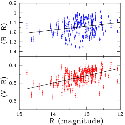
Figure 3: Upper and lower panels respectively show the (B-R) and (V-R) behaviour with respect to R band magnitude.

3.2 Radio Data

The radio flux density (in Jy) light curves on 36.8, 22.2, 14.5, 8 and 4.8 GHz are presented in the bottom panel of Figure 1. Data at 230 and 86 GHz are taken from Raiteri et al. (2013) and are shown in the middle panel. The most frequently sampled data were at 36.8 GHz; they show moderate activity until JD 2455750. After that one strong radio outburst occured at around JD 2455890 and a more moderate one is seen at JD 2455960. It can be seen from the figure that the light curves at all the radio frequencies exhibit similar behaviours and appear to be well correlated with each other during the first flare; this is the case at 36.8 and 14.5 GHz during the second, briefer, flare as well. However, at the radio frequency 22.2 GHz, there was a gap in the observations around JD 2455960 that is not clearly seen in the light curve as presented in Fig. 1, so that flare was not detected.

Table 1: Variability analysis parameters at radio wavelengths.

Freq.	$<$S$>$	$m_{0}$	m	$Y$	$\chi^{2}_{r}$	$N$	$\chi^{2}_{r~{}99.9\%}$	Telescope(s)
GHz(cm)	(Jy)	(%)	(%)	(%)
4.8(6.25)	4.30	1.00	1.63	5.73	6.362	48	1.76	UMRAO
8.0(3.75)	5.34	1.00	1.69	5.88	3.423	64	1.64	UMRAO
14.5(2.07)	5.23	1.00	1.91	6.48	5.209	124	1.44	UMRAO
22.2(1.35)	5.82	0.45	3.26	9.88	3.522	107	1.48	CrAO
36.8(0.81)	5.56	0.55	3.60	10.91	2.416	185	1.35	Finland, CrAO

$m$=variability index = $\sigma_{S}$/$<$S$>$,$\sigma_{S}$ standard deviation,
$m_{0}$ = variability index of the secondary calibrators,
$Y=3\sqrt{m^{2}-m_{0}^{2}}$ = bias corrected variability amplitude (see Fuhrmann et al. 2008),
$\chi^{2}_{r}$= reduced Chi-square,
$N$ = number of data points,
$\chi^{2}_{r~{}99.9\%}$ = reduced Chi-square corresponding to a significance level of 99.9$\%$.